For a non-ideal system, where the molar latent heat is no longer constant and where there is a substantial heat of mixing, the calculations become much more tedious.

For binary mixtures of this kind a graphical model has been developed by RUHEMANN, PONCHON, and SAVARIT, based on the use of an enthalpy-composition chart.

It is necessary to construct an enthalpy-composition diagram for particular binary system over a temperature range covering the two-phase vapor-liquid region at the pressure of the distillation.

The following data are needed:

1. Heat capacity as a function of temperature, composition and pressure.

2. Heat of mixing and dilution as a function of temperature and composition.

3. Latent heats of vaporization as a function of composition and pressure or temperature.

4. Bubble-point temperature as a function of composition and pressure.

n

iim hh (1)

In “regular” / ideal mixtures:

oiii hxh (2)

For gaseous / vapor mixtures at normal T and P:

n

iii

n

iim yhH (3)

Enthalpy of liquid:

Enthalpy-composition diagram

The equations used to calculate enthalpy of liquid and vapor are:

solBBAAmix Hhxhxh

solrefB,PBrefA,PAmix HTTCxTTCxh

mixmixmix hH

BBAAmix xx

(3)

(4)

(5)

(6)

EXAMPLE 2Devise an enthalpy-concentration diagram for the heptane-ethyl benzene system at 760 mm Hg, using the pure liquid at 0C as the reference state and assuming zero heat of mixing.

SOLUTION

heptane ethyl benzene TB (C) 136.2 98.5CP (cal/mole K) 51.9 43.4

(cal/mole) 7575 8600

t, C xH yH H EB

136.2 0.000 0.000 -- 1.00129.5 0.080 0.233 1.23 1.00122.9 0.185 0.428 1.19 1.02119.7 0.251 0.514 1.14 1.03116.0 0.335 0.608 1.12 1.05110.8 0.487 0.729 1.06 1.09106.2 0.651 0.834 1.03 1.15103.0 0.788 0.904 1.00 1.22100.2 0.914 0.963 1.00 1.2798.5 1.000 1.000 1.00 --

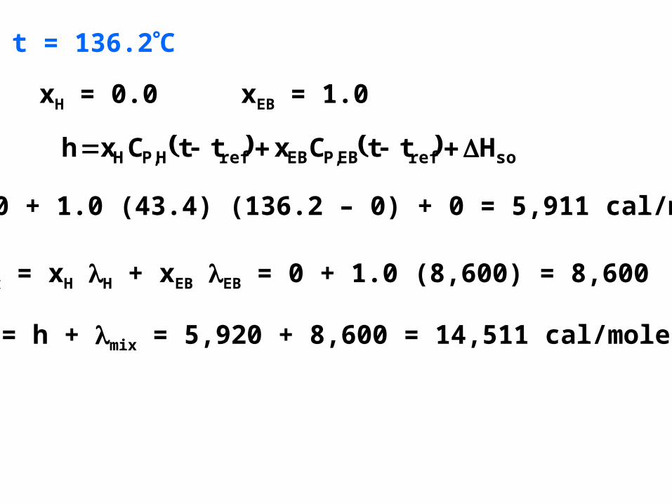
t = 136.2C

xH = 0.0 xEB = 1.0

solrefEB,PEBrefH,PH HttCxttCxh

= 0 + 1.0 (43.4) (136.2 – 0) + 0 = 5,911 cal/mole

mix = xH H + xEB EB = 0 + 1.0 (8,600) = 8,600

H = h + mix = 5,920 + 8,600 = 14,511 cal/mole

t = 129.5C

xH = 0.08 xEB = 0.92

solrefEB,PEBrefH,PH HttCxttCxh

= 0.08 (51.9) (129.5) + 0.92 (43.4) (136.2)

= 5,708 cal/mole

mix = xH H + xEB EB = 0.08 (7,575) + 0.92 (8,600) = 8,518

H = h + mix = 5,708 + 8,518 = 14,226 cal/mole

The computations are continued until the last point where xH = 1.0 and xEB = 0.0

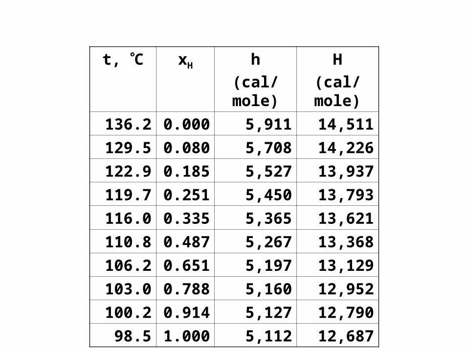
t, C xH h(cal/mole)

H(cal/mole)

136.2 0.000 5,911 14,511129.5 0.080 5,708 14,226122.9 0.185 5,527 13,937119.7 0.251 5,450 13,793116.0 0.335 5,365 13,621110.8 0.487 5,267 13,368106.2 0.651 5,197 13,129103.0 0.788 5,160 12,952100.2 0.914 5,127 12,790

98.5 1.000 5,112 12,687

0

2,000

4,000

6,000

8,000

10,000

12,000

14,000

16,000

18,000

20,000

0 0.2 0.4 0.6 0.8 1

x

HVapor

2 Phase

Liquid Saturated liquid

Saturated vapor

qF

V

L

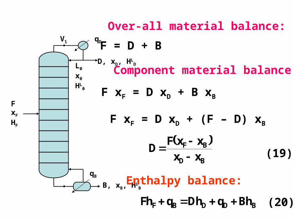
Over-all material balance:

F = V + L

F xF = V y + L x

F hF = V H + L h

(7)

(8)

(9)

The enthalpy-concentration diagram may be used to evaluate graphically the enthalpy and composition of streams added or separated.

Steady-state flow system with phase separation

and heat added

Component material balance

Enthalpy balance:

For adiabatic process, q = 0:

V (H – hF) = L (hF – h)

V (y – xF) = L (xF – x)

hhhH

VL

F

F

xxxy

VL

F

F

(10)

(12)

(11)

(13)

Substituting eq. (7) to (9) gives:

Substituting eq. (7) to (8) gives:

hLHVhLV F

xxxy

hhhH

F

F

F

F

(14)

Substituting eq. (12) to (13) gives:

xxhh

xyhH

F

F

F

F

Eq. (14) can be rearranged:

(15)

h

hF

H

L

F

V

x xFy

Enthalpy-concentration lines – adiabatic, q = 0

:isVFlineofslopeThe___

F

F

xyhH

:___

isFLlineofslopeThexxhh

F

F

According to eq. (15), the slopes of both lines are the same.

Since both lines go through the same point (F), the lines lie on the same straight line.

L

F

VH

hF

h

x xF y

A

B

LEVER-ARM RULE PRINCIPLE

hhhH

VL

F

F

Consider triangle LBV

VL

hhhH

BA

AV

LF

FV

F

F___

___

___

___

___

___

LF

FVVL

Similarly: ___

___

LV

LFFV

___

___

LV

FVFL

D, xD, HLD

B, xB, HLB

FxF

HF

qD

qB

V1

L0

x0

HL0

Over-all material balance:

F = D + B (16)

Component material balance:

F xF = D xD + B xB (17)

F xF = D xD + (F – D) xB (18)

BD

BF

xxxxF

D

(19)

Enthalpy balance:

(20)BDDBF hBqhDqhF

V1 = L0 + D (21)

V1 y1 = L0 x0 + D x0 (22)

Material balance around condenser:

Component material balance:

Enthalpy balance:

A

V1

L1

L0

DxD

qD

qD + V1 H1 = L0 h0 + D hD(23)

Combining eqs. (21) and (24):

D1

1DD0

hHHQh

DL

Internal reflux is shown as:

0DD

1DD

1

0

hQhHQh

VL

(25)

(26)

Designating:Dq

Q DD

V1 H1 = L0 h0 + D (hD – QD) (24)

Internal reflux between each plate, until a point in the column is reached where a stream is added or removed, can be shown as:

mDD

mDD

m

m

hQhHQh

VL

1

1(27)

A

Vm+1

Lm

L0

DxD

qD

m

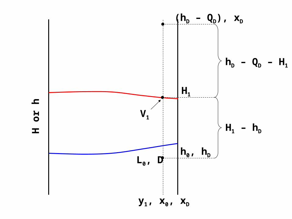
L0, Dh0, hD

V1

H1

(hD – QD), xD

hD – QD – H1

H1 – hD

y1, x0, xD

H o

r h

V1 = L0 + D (28)

y1 V1 = x0 L0 + yD D (29)

Material balance:

Component material balance:

Enthalpy balance:

qD + V1 H1 = L0 h0 + D HD (30)

Designating:Dq

Q DD

V1 H1 = L0 h0 + D (hD – QD) (31)

A

v1

v2

v3

vF

L1

L2

LF-1

L0

D, yD

FL

FxF

qD

Combining eqs. (28) and (30):

01

1DD0

hHHQH

DL

Internal reflux is shown as:

0DD

1DD

1

0

hQHHQH

VL

(32)

(33)

Internal reflux between each plate, until a point in the column is reached where a stream is added or removed, can be shown as:

mDD

1mDD

1m

m

hQHHQH

VL

(34)

h0, x0

V1

HD, yD

(HD – QD), yD

HD – QD – H1

H1 – h0

y1, x0, yD

H o

r h

D

V1

V3

Vn+1

L1

L2

Ln

L0

DxD

FL

qD

The material balance equation maybe rearranged in the from of difference:

L0 – V1 = L1 – V2 = L2 – V3

= . . . . = Lm – Vm+1

= – D =

(35)L0 – V1 = – D = n

V2

Combining eqs. (35) and (36):

xD = x (37)

For the component material balance:

L0 x0 – V1 y1 = L1 x1 – V2 y2

= L2 x2 – V3 y3 = . . . .

= Lm xm – Vm+1 ym+1

= – D xD = x

(36)L0 x0 – V1 y1 = – D xD = x

For the enthalpy balance:

L0 h0 – V1 H1 = L1 h1 –V2 H2 = L2 h2 –V3 H3 = . . . .

= Lm hm – Vm+1 Hm+1 = – D (hD – QD) = h

(38)

• These 3 independent equations [eqs. (35), (36), and (37)] can be written for rectifying section of the column between each plate.

• On the enthalpy scale and on the composition scale, the differences in enthalpy and in composition always pass through the same point, ([xD, (hD – QD)]

• This is designated as point , the difference point, and all lines corresponding to the combined material and enthalpy balance equations (operating line equations) for the rectifying section of the column pass through this intersection.

Combining eqs. (23) and (35):

h = hD – QD (39)

PLATE-TO-PLATE GRAPHICAL PROCEDURE FOR DETERMINING THE NUMBER OF EQUILIBRIUM STAGES:

1. Use R, xD, HD or hD to establish the location of point with x = xD and h = hD – QD or h = HD – QD

2. Use Equilibrium data alone to establish the point L1 at (x1, h1). Since L1 is assumed to be a saturated liquid, x1 must lie on the saturated-liquid line.

3. Draw the operating line between L1 and . This line intersects the saturated-vapor line at V2 (y2, H2).

4. Repeat steps 2 and 3 until the feed plate is reached.

x or y

H o

r h

V1V2

V3V4

DL1L2L3

(x, h)

BxB

qB

m

N

mL1mV

1MV

MV 1ML

ML

The material balance equation maybe rearranged in the from of difference:

MMMM VLBVL 11

...12 MM LL

1mm VL (40)

For the component material balance:

MMMMBMMMM yVxLxByVxL 1111

...1122 MMMM yVxL

xyVxL mmmm 11 (41)

Combining eqs. (40) and (42):

Bxx (42)

For the enthalpy balance:

(43)

MMMMBBMMMM HVhLQhBHVhL 1111

...1122 MMMM HVhL

hHVhL mmmm 11

Combining eqs. (40) and (43):

BB Qhh (44)

• These 3 independent equations [eqs. (40), (41), and (43)] can be written for stripping section of the column between each plate.

• On the enthalpy scale and on the composition scale, the differences in enthalpy and in composition always pass through the same point, [xB, (hB – QB)].

• This is designated as point , the difference point, and all lines corresponding to the combined material and enthalpy balance equations (operating line equations) for the stripping section of the column pass through this intersection.

F = D + B (45)

Combining eq. (45) with eqs. (35) and (40) gives:

F (46)

Equation (46) implies that lies on the extension of the straight line passing through F and .

QB is usually not known. It can be derived from over-all material balance:

PLATE-TO-PLATE GRAPHICAL PROCEDURE FOR DETERMINING THE NUMBER OF EQUILIBRIUM STAGES:

1. Draw a straight line passing through F and .

2. Draw a vertical straight line at xB all the way down until it intersects the extension of line F in

3. Assuming the reboiler to be an equilibrium stage, the vapor VM+1 is in equilibrium with the bottom stream.

4. Use equilibrium data alone to establish the value of ym+1 on the saturated-vapor line.

5. Draw the operating line between Lm(xm, hm) and VM+1. This line intersects the saturated-liquid line at

6. Repeat steps 4 and 5 until the feed plate is reached.

x or y

H o

r h

hB

1MV MV 1MV

Bx,

LM LM-1

D

B

F

qD

qB

V1

L0

• The construction may start from either side of the diagram, indicating either the condition at the top or the bottom of the column.

• Proceed as explained in previous slides.

• In either case, when an equilibrium tie line crosses the line connecting the difference points through the feed condition, the other difference point is used to complete the construction.

H o

r h

F

123456789

xF xDxB

H o

r h

V1

y1

x1

L1

EXAMPLE 3

Using the enthalpy-concentration diagram from Example 2, determine the following for the conditions in Example 1, assuming a saturated liquid feed.

a. The number of theoretical stages for an operating reflux ratio of R = L0/D = 2.5

b. Minimum reflux ratio L0/D.c. Minimum equilibrium stages at total reflux.d. Condenser duty feeding 10,000 lb of feed/hr, Btu/hr.e. Reboiler duty, Btu/hr.

SOLUTION

(a) From the graph: hD = h0 = 5,117 cal/mole H1 = 12,723 cal/mole

D1

1DD0

hHHQh

DL

117,5723,12723,12Q117,5

5.2 D

QD = – 26,621 cal/mole

h = hD – QD = 5,117 – (– 26,621) = 31,738 cal/mole

The coordinate of point is:

x = xD = 0.97

• Draw a straight line passing through and F.

• Extend the line until it intersects a vertical line passing through xB, at

• Draw operating lines and equilibrium lines in the whole column using the method explained in the previous slides.

Number of stages = 11

0

0.1

0.2

0.3

0.4

0.5

0.6

0.7

0.8

0.9

1

0 0.2 0.4 0.6 0.8 1

x

y

F

0

5,000

10,000

15,000

20,000

25,000

30,000

35,000

0 0.2 0.4 0.6 0.8 1

H

= 21,700 cal/mole

0

0.1

0.2

0.3

0.4

0.5

0.6

0.7

0.8

0.9

1

0 0.2 0.4 0.6 0.8 1

x

y

0

2,000

4,000

6,000

8,000

10,000

12,000

14,000

16,000

18,000

20,000

0 0.2 0.4 0.6 0.8 1

H

F

D1

1DD0

hHHQh

DL

D1

1

hHHh

117,5723,12723,12700,21

DL

min

0

= 1.18

(b)

0

0.1

0.2

0.3

0.4

0.5

0.6

0.7

0.8

0.9

1

0 0.2 0.4 0.6 0.8 1

x

y

0

2,000

4,000

6,000

8,000

10,000

12,000

14,000

16,000

18,000

20,000

0 0.2 0.4 0.6 0.8 1

H

F

1234567

N = 7

(c)

(d) hD – QD = h = 31,738 cal/mole

hD = 5,117 cal/mole

QD = – 26,621 cal/mole

Fmolelb103hrFlb000,10

FmoleDmole

426.0molecal

molelbBtu8.1molecal

621,26QD

= – 1,981,843 Btu/hr

(e) hB – QB = – 14,350 cal/mole

hB = 5,886 cal/mole

QB = 14,350 + 5,886 = 20,236 cal/mole

Fmolelb103hrFlb000,10

FmoleBmole

574.0molecal

molelbBtu8.1molecal

236,26QD

= 2,631,751 cal/mole