University of Texas at El Paso

Dep. of Mathematical Sciences

Mathematical Institute

Academy of Sciences

Czech Republic

On Some Aspects of the hp-FEMfor Time-Harmonic Maxwell’s Equations

Tomas Vejchodsky

vejchod@math.cas.cz

Pavel Solın

solin@utep.edu

Martin Zıtka

zitka@math.utep.edu

Midwest Numerical Analysis Conference,

May 20–22, 2005, University of Iowa

Time harmonic Maxwell’s equations

curl(µ−1

r curl E)− κ2εrE = F in Ω,

where

• curl = (∂/∂x2,−∂/∂x1)>

• curl E = ∂E2/∂x1 − ∂E1/∂x2

• Ω ⊂ R2

• µr = µr(x) ∈ R relative permeability

• εr = εr(x) ∈ C2×2 relative permittivity

• E = E(x) ∈ C2 phaser of the electric field intensity

• F = F(x) ∈ C2

• κ ∈ R the wave number

Time harmonic Maxwell’s equations + boundary conditions

curl(µ−1

r curl E)− κ2εrE = F in Ω

Perfect conducting boundary conditions:

E · τ = 0, on ΓP .

Impedance boundary conditions:

µ−1r curl E− iκλE · τ = g · τ on ΓI .

Here,

• τ = (−ν2, ν1)> positively oriented unit tangent vector

• λ = λ(x) > 0 impedance

• g = g(x) ∈ C2

Weak and FEM formulations

V = E ∈ H(curl,Ω) : ν × E = 0 on ΓP

E ∈ V : a(E,Φ) = F(Φ) ∀Φ ∈ V

Vh =Eh ∈ V : Eh|Kj ∈ P

pj(Kj) and

Eh · τk is continuous on each edge ek

Eh ∈ Vh : a(Eh,Φh) = F(Φh) ∀Φh ∈ Vh

a(E,Φ) =(µ−1

r curl E, curl Φ)− κ2 (εrE,Φ)− iκ 〈λE · τ,Φ · τ〉

F(Φ) = (F,Φ) + 〈g,Φ · τ〉

Eh =N∑jcj︸︷︷︸∈C

Ψj Ψj . . . hierarchic basis

Shape functions

Whitney functions:

ψe10 =

λ3n2

n2 · t1+

λ2n3

n3 · t1

ψe20 =

λ1n3

n3 · t2+

λ3n1

n1 · t2

ψe30 =

λ2n1

n1 · t3+

λ1n2

n2 · t3

First order functions:

ψe11 =

λ3n2

n2 · t1− λ2n3

n3 · t1

ψe21 =

λ1n3

n3 · t2− λ3n1

n1 · t2

ψe31 =

λ2n1

n1 · t3− λ1n2

n2 · t3

ti =

[−ni,2ni,1

]

Edge functions:

ψe1k =

2k − 1

kLk−1(λ3 − λ2)ψe1

1 −k − 1

kLk−2(λ3 − λ2)ψe1

0 ,

ψe2k =

2k − 1

kLk−1(λ1 − λ3)ψe1

1 −k − 1

kLk−2(λ1 − λ3)ψe1

0 ,

ψe2k =

2k − 1

kLk−1(λ2 − λ1)ψe1

1 −k − 1

kLk−2(λ2 − λ1)ψe1

0 , k = 2,3, . . .

Edge based bubble functions:

ψb,e1k = λ3λ2Lk−2(λ3 − λ2)n1,

ψb,e2k = λ1λ3Lk−2(λ1 − λ3)n2,

ψb,e3k = λ2λ1Lk−2(λ2 − λ1)n3, k = 2,3, . . .

Genuine bubble functions:

ψb,1n1,n2= λ1λ2λ3Ln1−1(λ3 − λ2)Ln2−1(λ2 − λ1)

[10

],

ψb,2n1,n2= λ1λ2λ3Ln1−1(λ3 − λ2)Ln2−1(λ2 − λ1)

[01

], 1 ≤ n1, n2

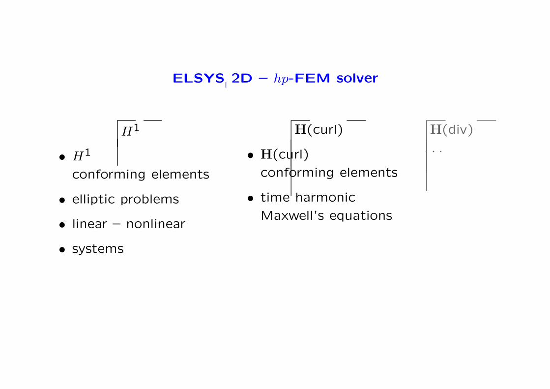
ELSYS 2D – hp-FEM solver

H1

• H1

conforming elements

• elliptic problems

• linear – nonlinear

• systems

H(curl)

• H(curl)

conforming elements

• time harmonic

Maxwell’s equations

H(div)

. . .

Structure of the C++ object oriented code

Project

Grid

Elements

→ VerticesNodes → DOFs

→ Reference Grid→ Quadrature

Shape Functions

Modularity of the code

common core × equation dependent modules

CProject H1Project

HcurlProjectCGrid

H1Grid

HcurlGrid

File names

CPU time

Input

Output

Quadrature

Assembling

Solving

Output

Error computation

Elements

Vertices

Nodes

Read Grid file

Preprocessing

Refinement

Boundary cond.

DOFs Allocation

Modularity of the code

CElement H1Element

HcurlElementsMatrix

Vertices

Neighours

Transformation

Edge orientations

Nodes – DOFs

Solution

Sparse matrices

Iterative solvers

Interface for:

– Trilinos

– PETSc

– UMFPACK

Example 1

‖E‖

ReE1 ReE2

u = r23 sin

(23θ + π

3

)

E = ∇u

E = 23r−1

3

cos(π6 + θ

3

)

sin(π6 + θ

3

)

F = −E

µr = 1

εr = I

κ = 1

λ = 1

g = . . .

Example 1

DOFs CPU time ‖Err‖H(curl)/‖E‖H(curl)

p = 0 2 758 400 11 min 26 s 0.156 %hp 2 732 0.55 s 0.138 %

Improvement 1 010× 1 247×

refinement 100

Example 1

DOFs CPU time ‖Err‖H(curl)/‖E‖H(curl)

p = 1 266 464 4 min 18 s 0.02612 %hp 5 534 2.67 s 0.02608 %

Improvement 48× 97×

refinement 22

Example 2 (P. Monk, 2003)

u = J23(r) cos

(23θ)

E = curlu

F = 0

µr = 1

εr = I

κ = 1

λ = 1

g = . . .

Example 2

DOFs CPU time ‖Err‖H(curl)/‖E‖H(curl)

p = 0 2 586 540 21 min 12 s 0.645 %hp 4 324 2.49 s 0.621 %

Improvement 598× 511×

refinement 10

Example 2

DOFs CPU time ‖Err‖H(curl)/‖E‖H(curl)

p = 1 827 664 7 min 3 s 1.068 %hp 2 624 1.51 s 0.966 %

Improvement 315× 280×

refinement 4

Outlook

• H1 and H(curl) conforming elements in 3D

• parallelization

• a posteriori error estimates

• automatic hp-adaptivity

• orthonormalization of the bubble functions

(investigation of the non-affine hierarchic elements)

• . . . . . . . . .

University of Texas at El Paso

Dep. of Mathematical Sciences

Mathematical Institute

Academy of Sciences

Czech Republic

Thank you for your attention.

Tomas Vejchodsky

vejchod@math.cas.cz

Pavel Solın

solin@utep.edu

Martin Zıtka

zitka@math.utep.edu

Midwest Numerical Analysis Conference,

May 20–22, 2005, University of Iowa