+

Excel WorkshopMarch 2012

04/20/23

+Let’s start with some Vocab

CellActive Cell

Cell grid

Formula Bar

Row

Column

Formula Builder

Range

04/20/23

+Text

•Enter text into Active Cell as you would with a word processer•Double-click the Cell Grid to make columns and rows “fit”•Formatting palette has font, size, alignment options available•But…keep it simple until your worksheet is done…

04/20/23

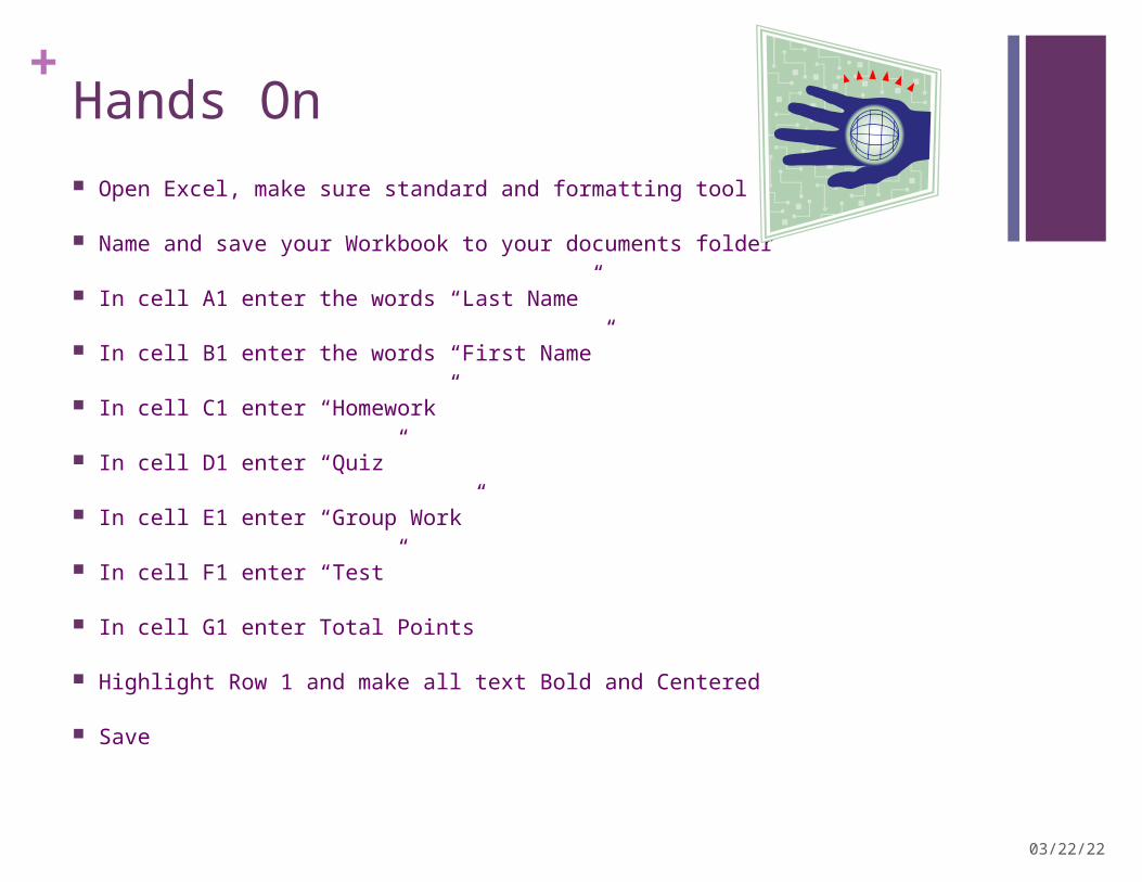
+Hands On Open Excel, make sure standard and formatting tool bars are on.

Name and save your Workbook to your documents folder

In cell A1 enter the words “Last Name”

In cell B1 enter the words “First Name”

In cell C1 enter “Homework”

In cell D1 enter “Quiz”

In cell E1 enter “Group Work”

In cell F1 enter “Test”

In cell G1 enter Total Points

Highlight Row 1 and make all text Bold and Centered

Save

04/20/23

+Your Worksheet Should Look Like:

04/20/23

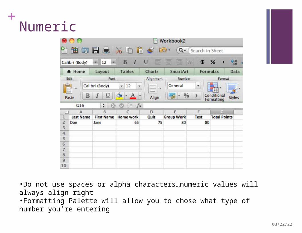
+Numeric

•Do not use spaces or alpha characters…numeric values will always align right•Formatting Palette will allow you to chose what type of number you’re entering

04/20/23

+Hands On

Add five student names

Use the tab key to move between cells

Add “scores” in columns C, D, E and F

Adjust all of the column widths so you can “see” what you just entered

04/20/23

+Your Worksheet Should Look Like:

04/20/23

+Using Mathematical Functions

All functions start with the = sign.

=sum(cell range) will add the values in that range of cells

=average(cell range) will average the data in a range

Use the Formula Builder

Or manually type in the formula. Your choice!

04/20/23

+Hands On

Open your spreadsheet

Click in cell G2 type =sum(

Click and hold in C2 and drag over to F2 close the parenthesis.

Click and hold on cell G2.

Highlight all of the other cells in column G that need an entry. Release the mouse.

Use Control+D key to fill the function into all cells (or use Edit>Fill>Down

Voila! Your formula is magically where you need it to be!

04/20/23

+Your Worksheet Should Look Like:

04/20/23

+Let’s find the Average Scores

Click in Cell H-1and type the word “Average”, Center and Bold it.

Click in H-2 and type =average(

Click and hold in cell C-2, and then drag across to cell F-2.

Close the parenthesis.

Fill down like you learned earlier for the Sum function.

04/20/23

+Hands On

Open your spreadsheet

Highlight column H by clicking on the letter H

Format>Conditional Formatting

Set Condition 1 so that if the value in column H (the average score) is between 0 and 70, the text will turn bold and red

Add a second condition and experiment! You can change cell color as well as text color.

04/20/23

+Making it pretty

Click on the File>Page Set Up function

Just like in MS Word, you can set margins and page orientation

Header/Footer will appear at the top/bottom of EVERY page

To make a row heading appear on every page, click the Sheet tab and then the “Rows to Repeat at the Top”. Click back out to your spreadsheet and highlight the rows you want to repeat.

04/20/23

+Let’s do some work!

Highlight from A1 to H6

Go up to Insert, and scroll down to chart

Select column graph.

Click on the Chart and go to the menu Chart, Source Data

Click on Switch Row/Column, see what happened?

04/20/23

+Insert A Graph

04/20/23

+Take some time to practice!

Questions and answers.

Please fill out evaluation form.

Don’t forget to sign the CEU form.

04/20/23