Introduction to the Use of MicroTran R

and other EMTP Versions

c 1998 by

Hermann W. Dommel

Department of Electrical and Computer EngineeringThe University of British Columbia

2356 Main MallVancouver, B. C.Canada, V6T 1Z4

Tel.: +1 (604) 822-2793, Fax: +1 (604) 822-5949Email: hermannd@ece.ubc.ca, WWW: http://www.ece.ubc.ca

These notes were �rst used in 1997/98 in a Graduate Course ELEC 553 "Advanced Power SystemsAnalysis". The help of the following graduate students in that course is gratefully acknowledged: S.

Bibian, B. D. Bonatto, J. D. Bull, J. Calvino-Fraga, N. Dai, Y. Duan, J. A. Hollman, F. A.Moreira, R. A. Rivas, T.-C. Yu.

Last revision: May 7, 1999.Web page created by: Daniel Lindenmeyer and Benedito Donizeti Bonatto.

Contents

1 Computer Programs for Electromagnetic Transients in Power Systems 3

2 Contributions from Research at UBC to Various Versions 4

3 Information for EMTP Users 5

4 Major Applications of MicroTran 6

5 Major Di�erences to Short-Circuit, Power Flow (Load Flow) and Stability Pro-grams 13

5.1 Di�erences to Short-Circuit Programs . . . . . . . . . . . . . . . . . . . . . . . . . . . 13

5.2 Di�erences to Power Flow Programs . . . . . . . . . . . . . . . . . . . . . . . . . . . 14

5.3 Di�erences to Stability Programs . . . . . . . . . . . . . . . . . . . . . . . . . . . . . 15

6 MicroTran Input Data 16

7 Case Studies: Short-Circuit in Single-Phase Network 17

7.1 Steady-state Solution Similar to Short-Circuit Programs . . . . . . . . . . . . . . . . 18

7.2 Transient Solution with Simple Single-Phase R-L Circuit . . . . . . . . . . . . . . . . 20

7.3 Transient Solution with Single-Phase R-L Circuit for Line . . . . . . . . . . . . . . . 22

7.4 Transient Solution with Single-Phase �-Circuit for Line . . . . . . . . . . . . . . . . . 23

7.5 Transient Solution with Single-Phase Distributed Parameter Line . . . . . . . . . . . 24

7.6 Comparison between R-L, �-Circuit, and Distributed Parameter Line Representations 25

7.7 Frequency Scan . . . . . . . . . . . . . . . . . . . . . . . . . . . . . . . . . . . . . . . 26

8 Case Studies: Short-Circuit in Three-Phase Network 28

8.1 Steady-State Solution Similar to Short-Circuit Programs . . . . . . . . . . . . . . . . 29

1

8.2 Transient Solution with Three-Phase R-L Circuit for Line . . . . . . . . . . . . . . . . 30

8.3 Transient Solution with Three-Phase �-Circuit for Line . . . . . . . . . . . . . . . . . 31

8.4 Transient Solution with Three-Phase Distributed Parameter Line . . . . . . . . . . . 33

8.5 Comparison between R-L, �-Circuit, and Distributed Parameter Line Representations 36

8.6 Transient Solution with Detailed Generator Model . . . . . . . . . . . . . . . . . . . . 36

8.7 Transient Solution with Actual Units . . . . . . . . . . . . . . . . . . . . . . . . . . . 38

8.8 Transient Solution for Simultaneous Three-Phase Short-Circuit . . . . . . . . . . . . . 39

8.9 Short-Circuits on HVDC Lines . . . . . . . . . . . . . . . . . . . . . . . . . . . . . . . 41

A Relationship between Phase Quantities and Sequence Quantities 42

Chapter 1

Computer Programs for Electromagnetic

Transients in Power Systems

EMTP versions

� Technical University Munich 1963 (�rst publication May 1964).

� BPA EMTP (probably no longer used by Bonneville Power Administration; may use ATP now);non-commercial. Was distributed for free because of Freedom of Information Act in U.S.A..

� UBC MicroTran R ; commercial. Most of it owned by University of British Columbia; dis-tributed by Microtran Power System Analysis Corporation in Vancouver, Canada.

� DCG/EPRI EMTP (DCG = Development Coordination Group, EPRI = Electric Power Re-search Institute in U.S.A.); commercial. Ontario Hydro is the commercializer.

� ATP (Alternative Transients Program of W. S. Meyer); free, but requires a license, which isnot available to everybody.

� NETOMAC (Siemens); commercial.

� Morgat and Arene (Electricit�e de France); commercial.

� EMTDC (Manitoba HVDC Research Centre); commercial.

� PSIM (H. Jin); commercial. Primarily for power electronics studies.

� SABER; commercial. For power electronics studies.

� SPICE, PSPICE, ...; commercial. Occasionally used for power electronics studies.

� ?

3

Chapter 2

Contributions from Research at UBC to

Various Versions

Contributions to BPA EMTP (and indirectly to DCG/EPRI EMTP and ATP), and insome cases to UBC version MicroTran:

� TACS of Laurent Dub�e (Transient Analysis of Control Systems).

� Multiphase untransposed transmission line with constant parameters of K. C. Lee (\CP linemodel").

� Frequency dependent transmission line of J. R. Mart��.

� Three-phase transformer models of H. W. Dommel and I. I. Dommel (\BCTRAN" in BPAEMTP, DCG/EPRI EMTP, and ATP; part of input preprocessor MTD in MicroTran).

� Synchronous machine model of V. Brandwajn (type 59 in DCG/EPRI EMTP and ATP).

� Synchronous machine data conversion of H. W. Dommel (earlier versions in BPA EMTP,DCG/EPRI EMTP, and ATP; latest version in MicroTran).

Contributions to DCG/EPRI EMTP:

� Underground cable models of L. Mart��.

� New line constants program and improved frequency dependent line model of J. R. Mart��.

4

Chapter 3

Information for EMTP Users

� EMTP Newsletter from 1979 to 1987, edited by H. W. Dommel (co-editor W. S. Meyer to 1984,D. Van Dommelen 1985 to 1987), with help from I. I. Dommel and G. Empereur.

� EMTP News from 1988 to 1993, edited by D. Van Dommelen, with help from G. Empereurand A. Laeremans.

� EMTP Review from 1987 to 1990, for users of DCG/EPRI EMTP, edited by W. F. Long.

� Harmonics and Transients Tech Notes, for members of PATH Users Group, Electrotek Con-cepts, Inc..

� Various User Groups set up or sanctioned by W. S. Meyer.

� CAN/AM EMTP News from 1994 (?) to now for ATP users, edited by W. S. Meyer andTsu-huei Liu.

� H. W. Dommel, EMTP Theory Book, 2nd edition. MicroTran R Power System Analysis Corp.,Vancouver, Canada, 1992. Latest update: April 1996.

� J. A. Martinez-Velasco, editor, Computer Analysis of Electric Power System Transients. IEEEPress, Piscataway, NJ, U.S.A., 1997.

� Specialized Conference IPST (International Power System Transients Conference), co-chairedby M. T. Correia de Barros and H. W. Dommel:

{ IPST'95 in August 1995 in Lisbon, Portugal.

{ IPST'97 in June 1997 in Seattle, Washington, U.S.A.

{ IPST'99 in June 1999 in Budapest, Hungary.

5

Chapter 4

Major Applications of MicroTran

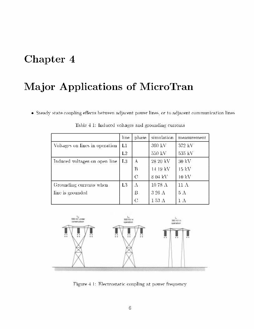
� Steady-state coupling e�ects between adjacent power lines, or to adjacent communication lines.

Table 4.1: Induced voltages and grounding currents

line phase simulation measurement

Voltages on lines in operation L1 360 kV 372 kV

L2 550 kV 535 kV

Induced voltages on open line L3 A 28.20 kV 30 kV

B 14.19 kV 15 kV

C 8.04 kV 10 kV

Grounding currents when L3 A 10.78 A 11 A

line is grounded B 3.26 A 5 A

C 1.53 A 1 A

Figure 4.1: Electrostatic coupling at power frequency

6

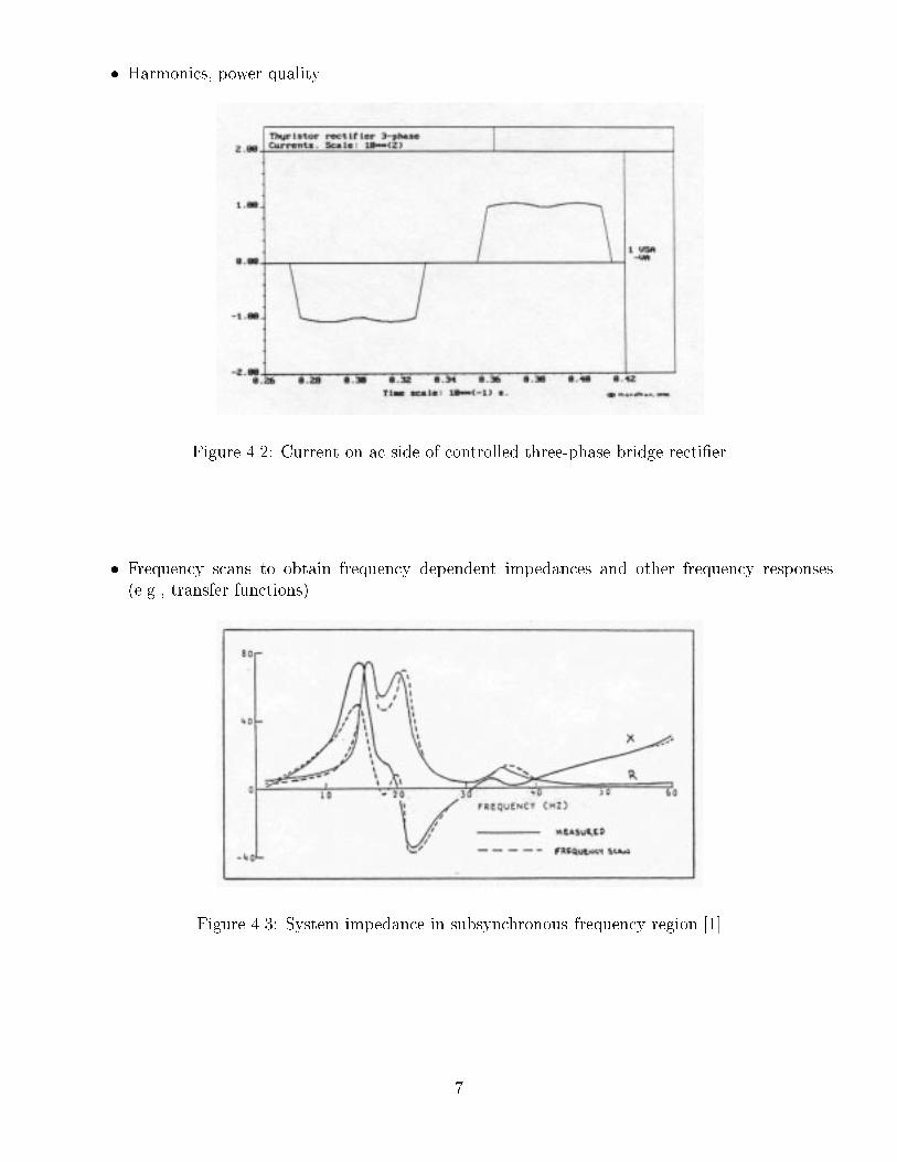
� Harmonics, power quality.

Figure 4.2: Current on ac side of controlled three-phase bridge recti�er

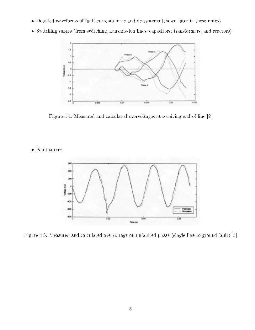
� Frequency scans to obtain frequency dependent impedances and other frequency responses(e.g., transfer functions).

Figure 4.3: System impedance in subsynchronous frequency region [1]

7

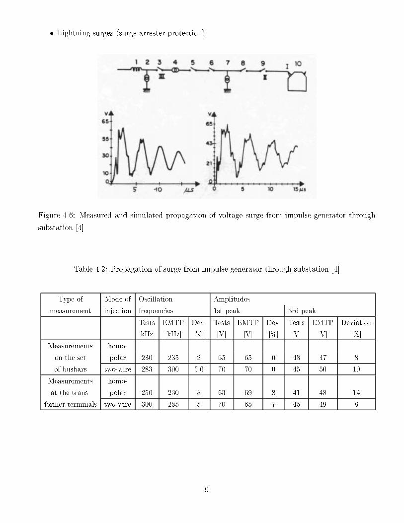
� Detailed waveforms of fault currents in ac and dc systems (shown later in these notes).

� Switching surges (from switching transmission lines, capacitors, transformers, and reactors).

Figure 4.4: Measured and calculated overvoltages at receiving end of line [2]

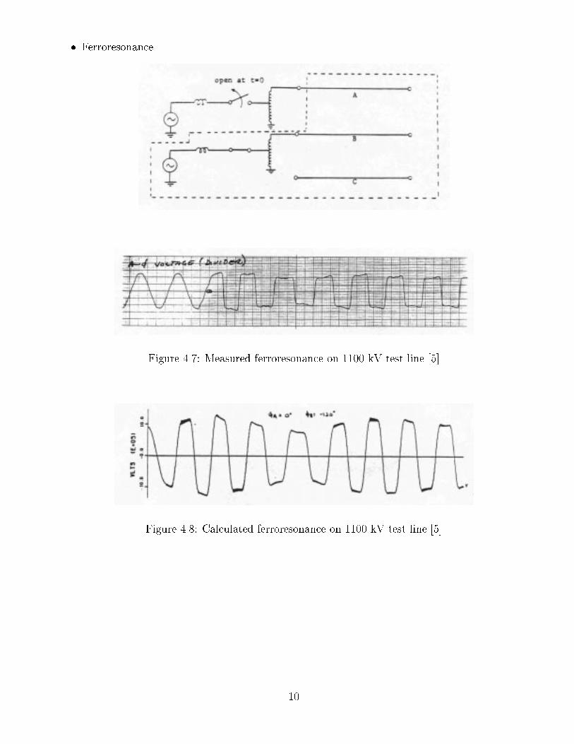
� Fault surges.

Figure 4.5: Measured and calculated overvoltage on unfaulted phase (single-line-to-ground fault) [3]

8

� Lightning surges (surge arrester protection).

Figure 4.6: Measured and simulated propagation of voltage surge from impulse generator through

substation [4]

Table 4.2: Propagation of surge from impulse generator through substation [4]

Type of Mode of Oscillation Amplitudes

measurement injection frequencies 1st peak 3rd peak

Tests EMTP Dev. Tests EMTP Dev. Tests EMTP Deviation

[kHz] [kHz] [%] [V] [V] [%] [V] [V] [%]

Measurements homo-

on the set polar 230 235 2 65 65 0 43 47 8

of busbars two-wire 283 300 5.6 70 70 0 45 50 10

Measurements homo-

at the trans- polar 250 230 8 63 69 8 41 48 14

former terminals two-wire 300 285 5 70 65 7 45 49 8

9

� Ferroresonance.

Figure 4.7: Measured ferroresonance on 1100 kV test line [5]

Figure 4.8: Calculated ferroresonance on 1100 kV test line [5]

10

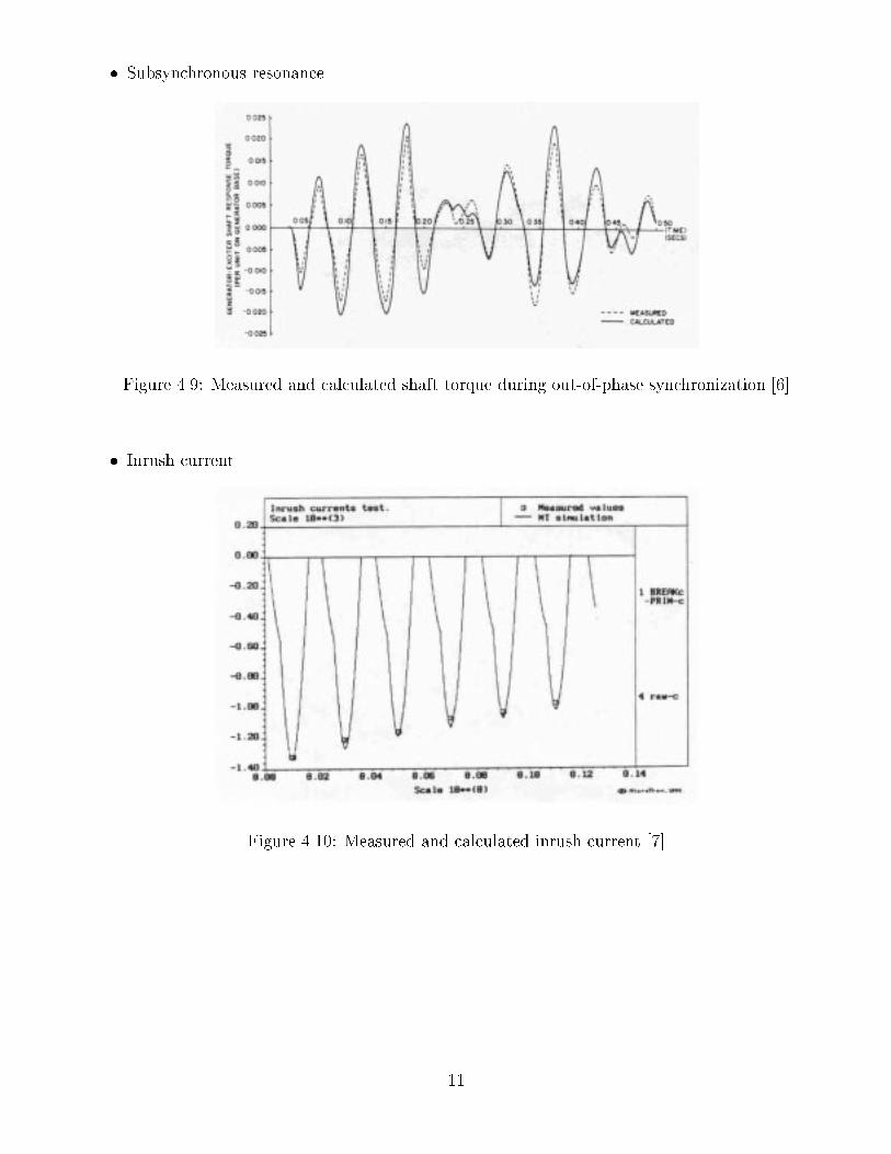
� Subsynchronous resonance.

Figure 4.9: Measured and calculated shaft torque during out-of-phase synchronization [6]

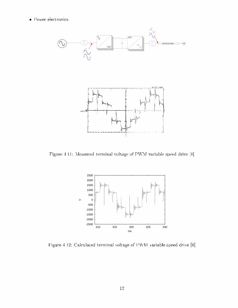
� Inrush current.

Figure 4.10: Measured and calculated inrush current [7]

11

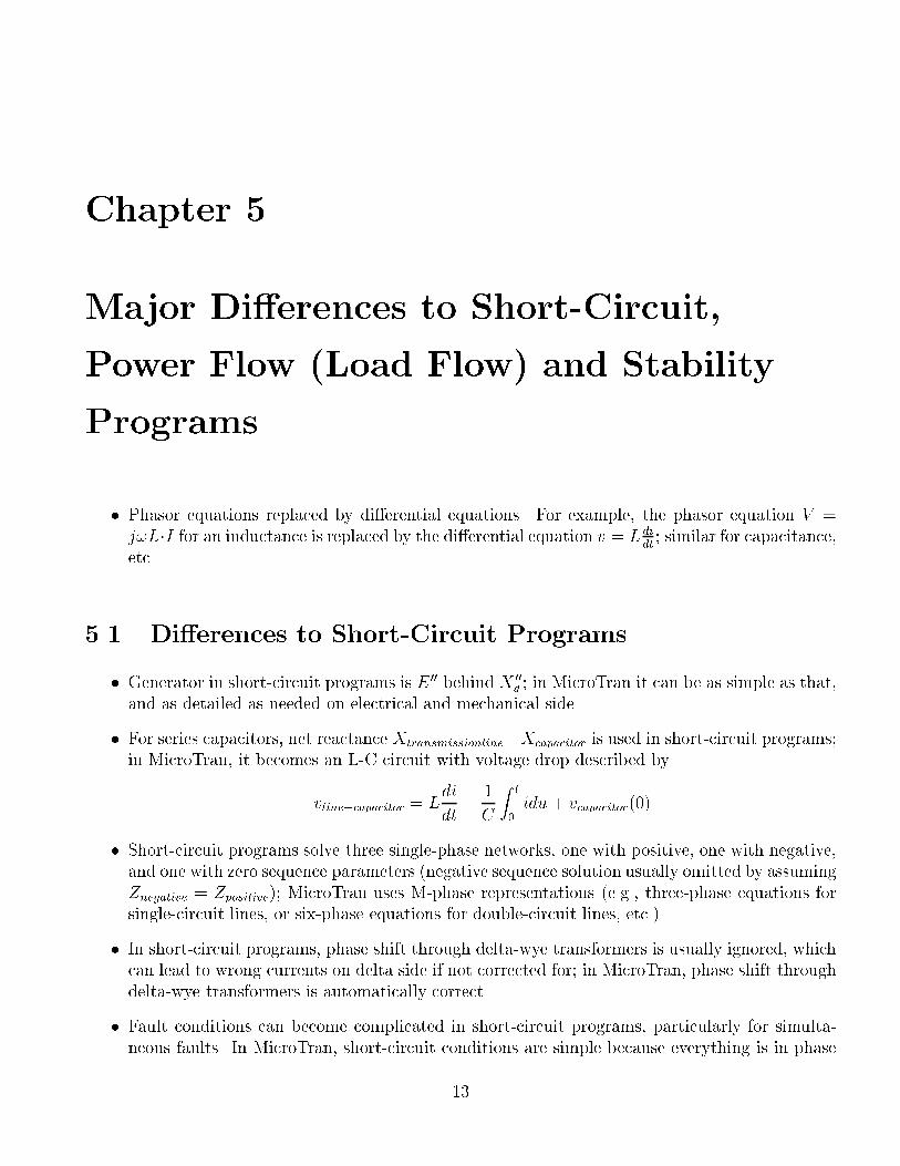
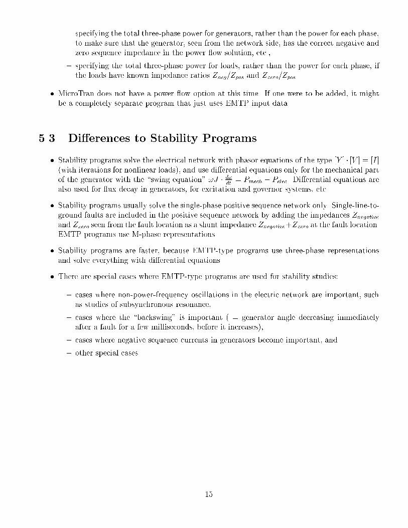
� Power electronics.

Electrical Cable I.M.

v

i

i

v

Figure 4.11: Measured terminal voltage of PWM variable speed drive [8]

-2500

-2000

-1500

-1000

-500

0

500

1000

1500

2000

2500

310 315 320 325 330

V

ms

Figure 4.12: Calculated terminal voltage of PWM variable speed drive [8]

12

Chapter 5

Major Di�erences to Short-Circuit,

Power Flow (Load Flow) and Stability

Programs

� Phasor equations replaced by di�erential equations. For example, the phasor equation V =j!L�I for an inductance is replaced by the di�erential equation v = L di

dt; similar for capacitance,

etc..

5.1 Di�erences to Short-Circuit Programs

� Generator in short-circuit programs is E 00 behind X 00d ; in MicroTran it can be as simple as that,

and as detailed as needed on electrical and mechanical side.

� For series capacitors, net reactance Xtransmissionline�Xcapacitor is used in short-circuit programs;in MicroTran, it becomes an L-C circuit with voltage drop described by

vline+capacitor = Ldi

dt+

1

C

Z t

0

idu+ vcapacitor(0)

� Short-circuit programs solve three single-phase networks, one with positive, one with negative,and one with zero sequence parameters (negative sequence solution usually omitted by assumingZnegative = Zpositive); MicroTran uses M-phase representations (e.g., three-phase equations forsingle-circuit lines, or six-phase equations for double-circuit lines, etc.).

� In short-circuit programs, phase shift through delta-wye transformers is usually ignored, whichcan lead to wrong currents on delta side if not corrected for; in MicroTran, phase shift throughdelta-wye transformers is automatically correct.

� Fault conditions can become complicated in short-circuit programs, particularly for simulta-neous faults. In MicroTran, short-circuit conditions are simple because everything is in phase

13

quantities (e.g., Va = 0 for a short from phase a to ground); simultaneous faults are easy inMicroTran. Example: Va�high = 0 and Vb�low = Vc�low for short \a" to ground on high sideand short between \b" and \c" on low side; high side fault represented by a closed switch from\a" to ground, and low side fault by a switch between \b-low" and \c-low".

� MicroTran produces the following e�ects, which cannot be obtained from short-circuit pro-grams:

{ decaying dc o�set in fault current,

{ decaying ac amplitude with detailed generator model,

{ more than one frequency with series capacitors,

{ di�erent X/R ratios automatically accounted for.

5.2 Di�erences to Power Flow Programs

� EMTP programs use steady-state solutions for the system of linear node equations , either

{ to get initial conditions for transient simulations, or

{ to get steady-state solutions at one frequency, or at many frequencies in so-called frequencyscans.

� You can de�ne voltage and/or current sources for these solutions, by specifying the sourceswith respect to magnitude and angle.

� You cannot specify real and reactive power, or real power and voltage magnitude, in theselinear solutions.

� The incentive for power ow solutions with EMTP-type programs came from the fact thatthese programs allow users to set up cases in great detail, such as

{ untransposed lines (single-circuit, double-circuit, etc.),

{ single-phase distribution lines connected to three-phase substations,

{ etc.

� Such cases cannot be solved with classical power ow programs, which assume that the powersystem is completely "balanced" (all voltages and currents symmetrical) and represented bythe single-phase positive sequence network only.

� In the ATP version of the EMTP, a power ow option was added which uses a Gauss-Seideltype iteration method. This method is unreliable with respect to convergence, and only worksfor some cases.

� In the DCG/EPRI version of the EMTP, a power ow option was added which uses New-ton's iteration method. This method is much more reliable. This option also takes physicalconstraints into account, such as [9]:

14

{ specifying the total three-phase power for generators, rather than the power for each phase,to make sure that the generator, seen from the network side, has the correct negative andzero sequence impedance in the power ow solution, etc.,

{ specifying the total three-phase power for loads, rather than the power for each phase, ifthe loads have known impedance ratios Zneg=Zpos and Zzero=Zpos.

� MicroTran does not have a power ow option at this time. If one were to be added, it mightbe a completely separate program that just uses EMTP input data.

5.3 Di�erences to Stability Programs

� Stability programs solve the electrical network with phasor equations of the type [Y ] � [V ] = [I](with iterations for nonlinear loads), and use di�erential equations only for the mechanical partof the generator with the \swing equation" !J � d!

dt= Pmech � Pelec. Di�erential equations are

also used for ux decay in generators, for excitation and governor systems, etc.

� Stability programs usually solve the single-phase positive sequence network only. Single-line-to-ground faults are included in the positive sequence network by adding the impedances Znegative

and Zzero seen from the fault location as a shunt impedance Znegative+Zzero at the fault location.EMTP programs use M-phase representations.

� Stability programs are faster, because EMTP-type programs use three-phase representationsand solve everything with di�erential equations.

� There are special cases where EMTP-type programs are used for stability studies:

{ cases where non-power-frequency oscillations in the electric network are important, suchas studies of subsynchronous resonance,

{ cases where the \backswing" is important ( = generator angle decreasing immediatelyafter a fault for a few milliseconds, before it increases),

{ cases where negative sequence currents in generators become important, and

{ other special cases.

15

Chapter 6

MicroTran Input Data

� Rarely p.u., usually actual quantities. See SSR fact sheet for comparison between two ap-proaches. Careful if nonlinearities!

� �t related to fmax of interest. Unfortunately not automatically chosen.

� Basic data:

{ type 0 branch: R-L-C

{ type 1,2,3 ... branches: M-phase symmetric �-circuit (type 51, 52, 53 ... for input withhigher accuracy)

{ type -1,-2,-3 ... branches: M-phase distributed parameter line

{ nonlinear R,L

{ switches, diodes, thyristors

{ sources

16

Chapter 7

Case Studies: Short-Circuit in

Single-Phase Network

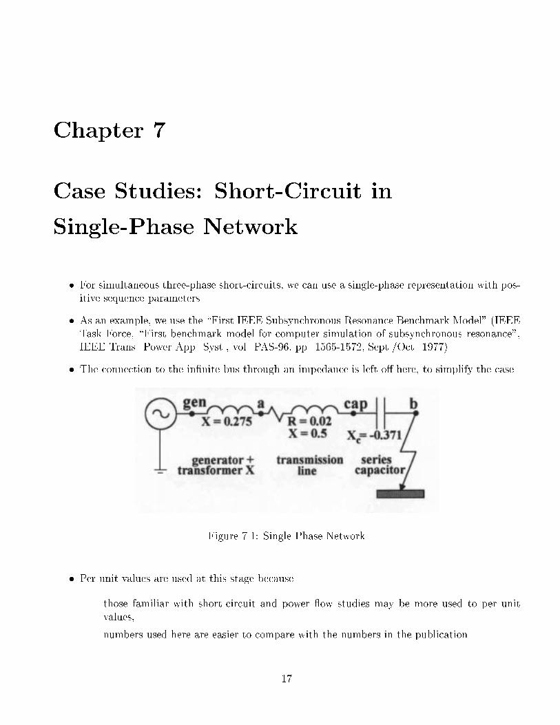
� For simultaneous three-phase short-circuits, we can use a single-phase representation with pos-itive sequence parameters.

� As an example, we use the \First IEEE Subsynchronous Resonance Benchmark Model" (IEEETask Force, \First benchmark model for computer simulation of subsynchronous resonance",IEEE Trans. Power App. Syst., vol. PAS-96, pp. 1565-1572, Sept./Oct. 1977).

� The connection to the in�nite bus through an impedance is left o� here, to simplify the case.

Figure 7.1: Single-Phase Network

� Per unit values are used at this stage because

{ those familiar with short-circuit and power ow studies may be more used to per unitvalues,

{ numbers used here are easier to compare with the numbers in the publication.

17

� In general, actual units are better for transient studies, and we will switch to actual units lateron.

� With XOPT = 60, input for inductive branches will be as reactance !L in at 60 Hz.

� The generator is represented as a voltage source E 00 behind X 00d . Assume Vgen = 1:0 p:u: (RMS)

for E 00.

� The values for this single-phase case are the positive sequence values.

� The fault resistance is assumed to be 0.04 p.u. In the IEEE benchmark case, it is inductive,but a resistive fault impedance is more realistic. Maybe the impedance in the IEEE benchmarkcase represented a short line from the bus to the fault location.

7.1 Steady-state Solution Similar to Short-Circuit Pro-

grams

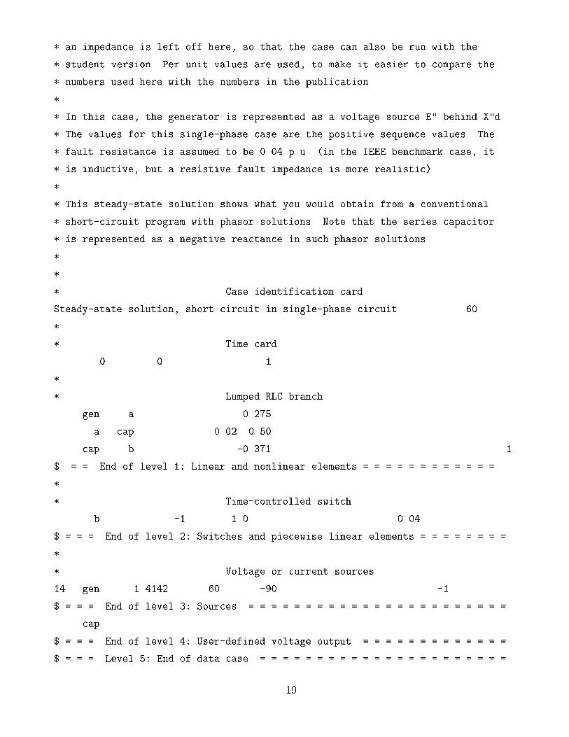
� Data �le: 1 STEADY.DAT

� This steady-state solution shows what you would obtain from a conventional short-circuitprogram with phasor solutions, namely Ifault =

VprefaultRtotal+j!Ltotal

= 1:00:06+j0:404

p:u:, or jIfaultj =2:448 p:u:.

� Note that the series capacitor is represented as a negative reactance in such phasor solutions.

� Leave �t and tmax empty (or set them zero). Then only a steady-state solution will be per-formed.

� Use tstart = �1:0 (any negative number) in the source data to indicate that source is alreadypresent in steady state before transient simulation begins at t = 0.

� Use tclose = �1:0 in the data for the switch simulating the fault, to indicate that the switch isalready closed in steady state before transient simulation begins at t = 0.

� Ask for fault current with \1" in column 80 of series capacitor data line (do not ask for switchcurrent because switch current from steady-state solution is not available at this time).

� If you want a complete steady-state output, insert \1" in column 38 of time data line.

* File "1_STEADY.DAT".

* To demonstrate the various ways of calculating short-circuit currents, the

* "First IEEE Subsynchronous Resonance Benchmark Model" is used as an example

* (IEEE Task Force, "First benchmark model for computer simulation of sub-

* synchronous resonance", IEEE Trans. Power App. Syst., vol. PAS-96,

* pp. 1565-1572, Sept./Oct. 1977). The connection to the infinite bus through

18

* an impedance is left off here, so that the case can also be run with the

* student version. Per unit values are used, to make it easier to compare the

* numbers used here with the numbers in the publication.

*

* In this case, the generator is represented as a voltage source E" behind X"d.

* The values for this single-phase case are the positive sequence values. The

* fault resistance is assumed to be 0.04 p.u. (in the IEEE benchmark case, it

* is inductive, but a resistive fault impedance is more realistic).

*

* This steady-state solution shows what you would obtain from a conventional

* short-circuit program with phasor solutions. Note that the series capacitor

* is represented as a negative reactance in such phasor solutions.

*

*

* . . . . . . . Case identification card

Steady-state solution, short circuit in single-phase circuit 60

*

* . . . . . . . Time card

0. 0. 1

*

* . . . . . . . Lumped RLC branch

gen a 0.275

a cap 0.02 0.50

cap b -0.371 1

$ = = End of level 1: Linear and nonlinear elements = = = = = = = = = = = =

*

* . . . . . . . Time-controlled switch

b -1. 1.0 0.04

$ = = = End of level 2: Switches and piecewise linear elements = = = = = = = =

*

* . . . . . . . Voltage or current sources

14 gen 1.4142 60. -90. -1.

$ = = = End of level 3: Sources = = = = = = = = = = = = = = = = = = = = = = =

cap

$ = = = End of level 4: User-defined voltage output = = = = = = = = = = = = =

$ = = = Level 5: End of data case = = = = = = = = = = = = = = = = = = = = = =

19

7.2 Transient Solution with Simple Single-Phase R-L Cir-

cuit

� Data �le: 1 SIMPLE.DAT

� Change �t to 50 �s, and tmax to 0.1 s. Step size �t is related to maximum frequency whichyou expect or want to see in the results: fmax = 1

8�t, if you want 8 points per cycle at the

highest frequency.

� Change tclose of switch to 0, so that fault is initiated at t = 0 (topen = 1:0 will keep switchclosed during transient solution to tmax = 0:1s).

� Ask for fault current output with \1" in column 80 of switch data line.

� Ask for capacitor current and voltage with \3" in column 80 of capacitor data line.

� If it is a simple series connection of resistances and inductances (assuming that the seriescapacitor simply decreases the line inductance, which is not correct as shown in the next case),then there is an exact solution for the �rst-order di�erential equation of the R-L circuit.

� With a voltage source of v(t) = Vmax sin(!t+ �), we obtain:

i(t) =Vmaxq

R2total + (!Ltotal)2

hsin(!t+ �� )� sin(�� ) � e� t

T

i;

where = tan�1�!LtotalRtotal

�, T = Ltotal

Rtotal, Rtotal = 0:06 p:u:, !Ltotal = 0:404 p:u:, f = 60Hz.

� For �� = 0�, there is no dc o�set. For �� = 90�, there is maximum dc o�set.

� In high voltage systems, R� !L. In that case, maximum dc o�set occurs when the voltage isjust going through zero, v(t) = Vmax sin(!t).

� With maximum dc o�set, the peak current is twice as high as without dc o�set if the decay isvery slow, or somewhat less than twice as high with faster decay. As seen from above equation,the decay time constant is 1

!� Xtotal

Rtotal.

� Knowing the dc o�set is important because it

{ increases the mechanical forces between busbars carrying the current and return currentby a factor of up to 4,

{ increases the power dissipation i2 � Rarc in the circuit breaker arc by a factor of up to 4,and

20

{ may prevent zero crossings for the �rst few cycles in three-phase short circuits close togenerator terminals (see notes "Simple Sources and Machine Models"); in reality, the arcresistance will probably create enough decay to create zero crossings early enough for thecircuit breaker to operate.

� The dc o�set in the fault current is taken into account in the circuit breaker standards.

{ Older standards provided data for the in uence of the decaying dc o�set on circuit breakerratings as functions of X/R ratios.

{ Newer standards use symmetrical current ratings (dc o�set implicitly assumed), and showratios of asymmetrical to symmetrical interrupting capabilities as a function of contactparting time.

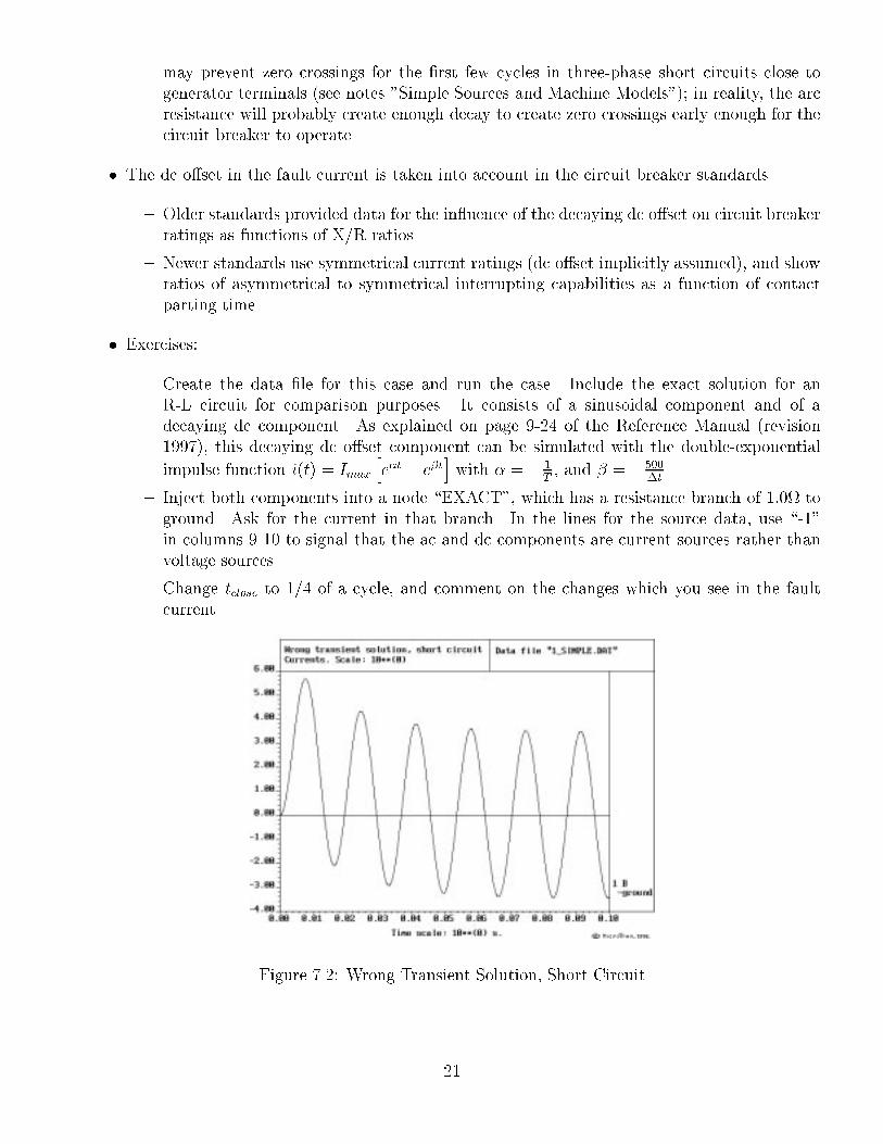
� Exercises:

{ Create the data �le for this case and run the case. Include the exact solution for anR-L circuit for comparison purposes. It consists of a sinusoidal component and of adecaying dc component. As explained on page 9-24 of the Reference Manual (revision1997), this decaying dc o�set component can be simulated with the double-exponential

impulse function i(t) = Imax

he�t � e�t

iwith � = � 1

T, and � = �500

�t.

{ Inject both components into a node \EXACT", which has a resistance branch of 1:0 toground. Ask for the current in that branch. In the lines for the source data, use \-1"in columns 9-10 to signal that the ac and dc components are current sources rather thanvoltage sources.

{ Change tclose to 1/4 of a cycle, and comment on the changes which you see in the faultcurrent.

Figure 7.2: Wrong Transient Solution, Short Circuit

21

7.3 Transient Solution with Single-Phase R-L Circuit for

Line

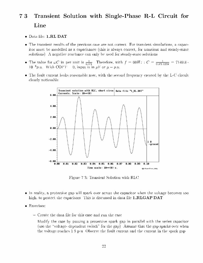
� Data �le: 1 RL.DAT

� The transient results of the previous case are not correct. For transient simulations, a capac-itor must be modelled as a capacitance (this is always correct, for transient and steady-statesolutions). A negative reactance can only be used for steady-state solutions.

� The value for !C in per unit is 1

0:371. Therefore, with f = 60Hz : C = 1

0:371�120� = 7149:8 �10�6p:u:. With COPT = 0, input is in �F or �� p:u:

� The fault current looks reasonable now, with the second frequency created by the L-C circuitclearly noticeable.

Figure 7.3: Transient Solution with RLC

� In reality, a protective gap will spark over across the capacitor when the voltage becomes toohigh, to protect the capacitors. This is discussed in data �le 1 RLGAP.DAT.

� Exercises:

{ Create the data �le for this case and run the case.

{ Modify the case by putting a protective spark gap in parallel with the series capacitor(use the \voltage- dependent switch" for the gap). Assume that the gap sparks over whenthe voltage reaches 1.8 p.u. Observe the fault current and the current in the spark gap.

22

{ Disable the critical damping adjustment scheme (CDA) with "1" in column 68 of the timedata line, and change �t to 1ms (larger �t shows numerical oscillations clearer). Observethe numerical oscillations in the gap current and capacitor current (one should be thenegative of the other).

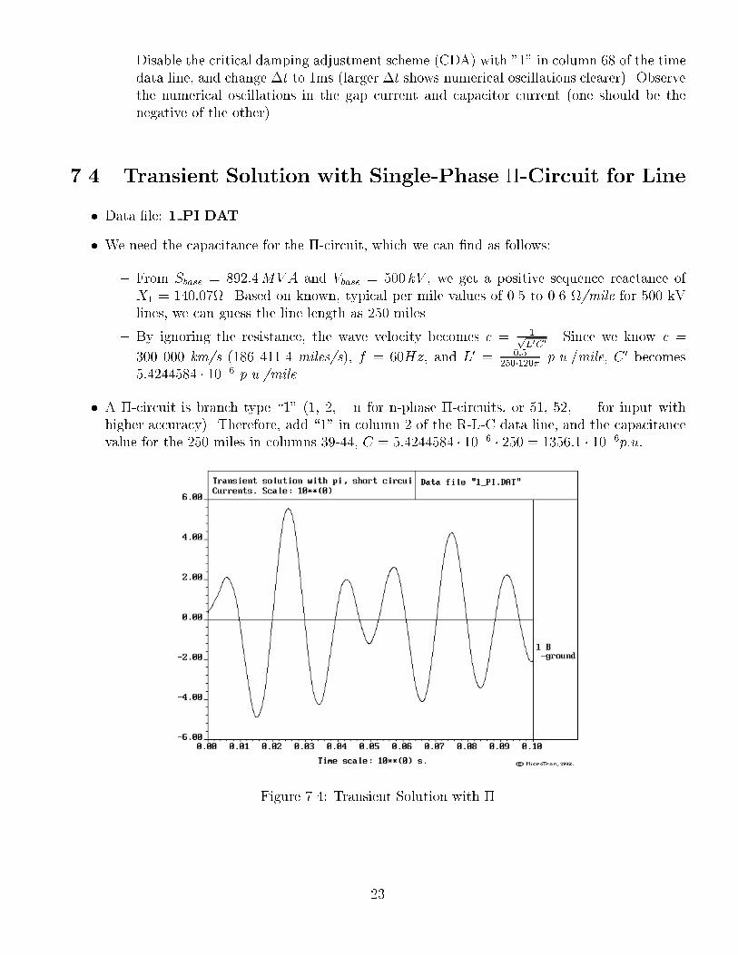
7.4 Transient Solution with Single-Phase �-Circuit for Line

� Data �le: 1 PI.DAT

� We need the capacitance for the �-circuit, which we can �nd as follows:

{ From Sbase = 892:4MVA and Vbase = 500 kV , we get a positive sequence reactance ofX1 = 140:07. Based on known, typical per mile values of 0.5 to 0.6 /mile for 500 kVlines, we can guess the line length as 250 miles.

{ By ignoring the resistance, the wave velocity becomes c = 1pL0C0

. Since we know c =

300 000 km/s (186 411.4 miles/s), f = 60Hz, and L0 = 0:5250�120� p.u./mile, C 0 becomes

5:4244584 � 10�6 p.u./mile.

� A �-circuit is branch type \1" (1, 2, ...n for n-phase �-circuits, or 51, 52, ... for input withhigher accuracy). Therefore, add \1" in column 2 of the R-L-C data line, and the capacitancevalue for the 250 miles in columns 39-44, C = 5:4244584 � 10�6 � 250 = 1356:1 � 10�6p:u:

Figure 7.4: Transient Solution with �

23

� If we were to move the fault location to the end of the transmission line in node \cap", wewould short-circuit the shunt capacitance at node \cap" of the �-circuit. If the fault impedancewere zero, this would theoretically produce an in�nite current spike of in�nitely small duration.Without the critical damping adjustment scheme for the suppression of numerical oscillations(CDA), numerical oscillations would appear in the fault current. See data �le 1 PINUM.DATfor this case with numerical oscillations in the current.

� Exercises:

{ Create the data �le for this case and run the case.

{ Move the fault location to node \cap", assume zero fault resistance, and observe the faultcurrent.

{ Put a \1" in column 68 of the data line for �t, etc., to bypass CDA, and observe the faultcurrent again.

{ Re-run it again with tclose changed to 1/4 cycle. Observe the fault current again.

7.5 Transient Solution with Single-Phase Distributed Pa-

rameter Line

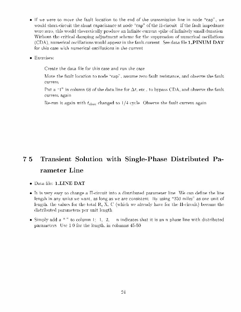
� Data �le: 1 LINE.DAT

� It is very easy to change a �-circuit into a distributed parameter line. We can de�ne the linelength in any units we want, as long as we are consistent. By using \250 miles" as one unit oflength, the values for the total R, X, C (which we already have for the �-circuit) become thedistributed parameters per unit length.

� Simply add a \-" to column 1; -1, -2, ...-n indicates that it is an n-phase line with distributedparameters. Use 1.0 for the length, in columns 45-50.

24

Figure 7.5: Transient Solution with Distributed Parameters

� Without CDA, numerical oscillations can occur in the fault current with the �-circuit model.With the distributed parameter model, there are no numerical oscillations, because node "cap"does not have a lumped shunt capacitance, but sees travelling waves from the transmission lineinstead. See data �le 1 LINUM.DAT.

� Exercises:

{ Create the data �le for this case and run the case.

{ Put a \1" in column 68 of the data line for �t, etc., to bypass CDA, and observe the faultcurrent again.

7.6 Comparison between R-L, �-Circuit, and Distributed

Parameter Line Representations

� Exercises:

{ Superimpose the fault currents from the three line models on the same plot.

{ Comment on the similarities and di�erences.

� The fault current is reasonably accurate with all three representations.

� The distributed parameter line model is the correct model, but it can only be used as long asthe travel time � (1.34 ms in this case) is larger than the step size �t (50 �s in this case).

25

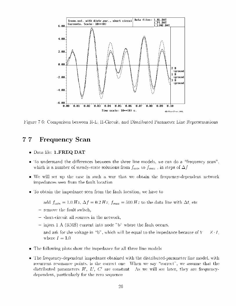
Figure 7.6: Comparison between R-L, �-Circuit, and Distributed Parameter Line Representations

7.7 Frequency Scan

� Data �le: 1 FREQ.DAT

� To understand the di�erences between the three line models, we can do a \frequency scan",which is a number of steady-state solutions from fmin to fmax , in steps of �f .

� We will set up the case in such a way that we obtain the frequency-dependent networkimpedances seen from the fault location.

� To obtain the impedance seen from the fault location, we have to

{ add fmin = 1:0Hz, �f = 0:2Hz, fmax = 500Hz to the data line with �t, etc.

{ remove the fault switch,

{ short-circuit all sources in the network,

{ inject 1 A (RMS) current into node "b" where the fault occurs,

{ and ask for the voltage in \b", which will be equal to the impedance because of V = Z � I,where I = 1:0.

� The following plots show the impedance for all three line models.

� The frequency-dependent impedance obtained with the distributed-parameter line model, withrecurrent resonance points, is the correct one. When we say \correct", we assume that thedistributed parameters R0, L0, C 0 are constant. As we will see later, they are frequency-dependent, particularly for the zero sequence.

26

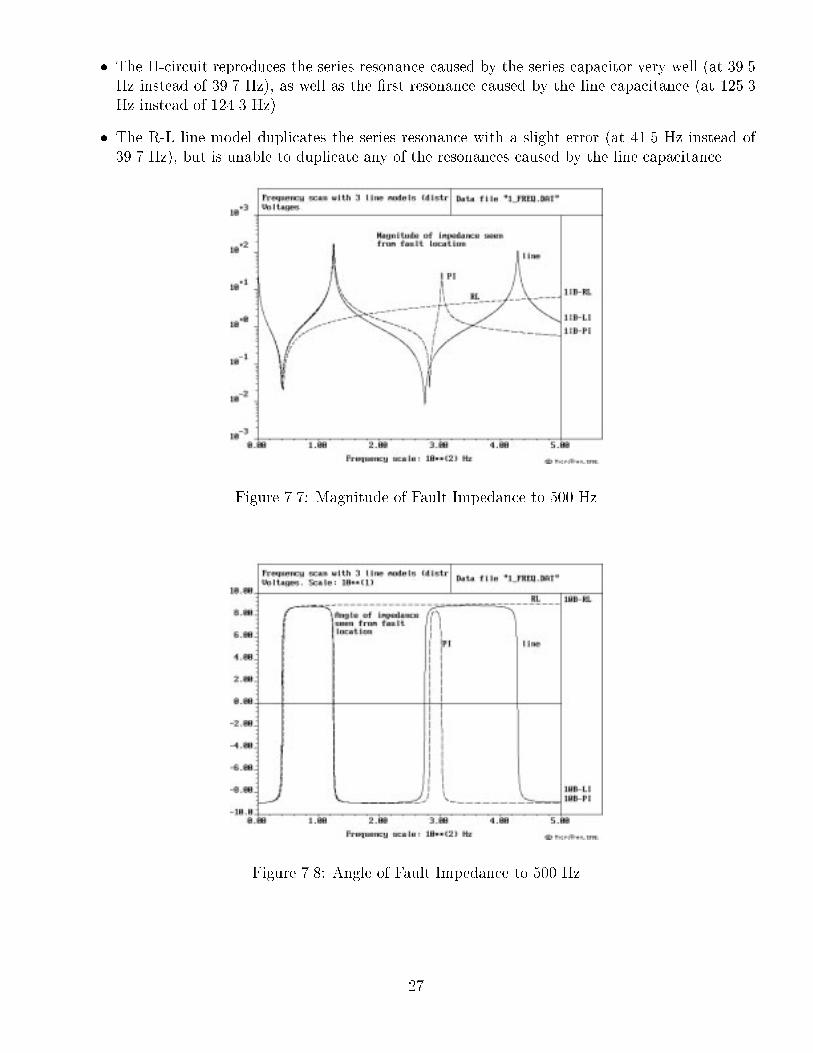
� The �-circuit reproduces the series resonance caused by the series capacitor very well (at 39.5Hz instead of 39.7 Hz), as well as the �rst resonance caused by the line capacitance (at 125.3Hz instead of 124.3 Hz).

� The R-L line model duplicates the series resonance with a slight error (at 41.5 Hz instead of39.7 Hz), but is unable to duplicate any of the resonances caused by the line capacitance.

Figure 7.7: Magnitude of Fault Impedance to 500 Hz

Figure 7.8: Angle of Fault Impedance to 500 Hz

27

Chapter 8

Case Studies: Short-Circuit in

Three-Phase Network

� In addition to the positive sequence parameters, we also need the zero sequence parametersnow:

{ The zero sequence source reactance is the transformer reactance alone, because the trans-former is seen as an internal short on the delta side, and disconnected from the generator,X0 = 0:14 p:u:

{ The zero sequence line impedance is R0 = 0:5 p:u:, X0 = 1:56 p:u:

� We assume a single-line-to-ground fault in phase A of node \b". In high-voltage transmissionsystems, 90 % or so of all faults are single-line-to-ground.

� We will also look at the overvoltages in the unfaulted phases at node \b". The steady-stateovervoltages do not depend on the \fault-initiation angle" (angle where fault occurs, countedfrom zero crossing of the pre-fault sinusoidal voltage). The transient overvoltages depend verymuch on the fault initiation angle. They are largest in one of the unfaulted phases if the faultoccurs when the voltage is just at its maximum. We therefore use tclose = 0:0041667 s (faultinitiation angle = 90�).

� With a fault initiation angle of 90�, there is little dc o�set in the fault current. The circuitbreaker duty is therefore less than with a fault initiation angle of 0�, but the latter produceshigher transient overvoltages.

� Transient overvoltages during line energization can be minimized with controlled closing (clos-ing when the voltages are more or less equal on both sides of the circuit breaker contact). Thedisadvantage is the maximum dc o�set in the fault current if we happen to re-close into apermanent fault.

28

8.1 Steady-State Solution Similar to Short-Circuit Pro-

grams

� Data �le: 3 STEADY.DAT

� This steady-state solution shows what you would obtain from a conventional short-circuitprogram with phasor solutions.

� While short-circuit programs usually work with positive and zero sequence networks, MicroTranworks with phase quantities. See Appendix A for relationship between sequence and phasequantities.

� Replace the single-phase R-L branch with three coupled branches (use the �-circuit branchtypes 1, 2, 3, or branch types 51, 52, 53 for higher accuracy input, for the three coupledbranches, and leave the �eld for the capacitances blank). When you use the pre-processor\MTD", there is a \device" entry form for symmetric �-circuits which allows you to inputzero and positive sequence parameters. If you have a version of MTD which creates cascadeconnections of �-circuits, make certain that you specify the number of sections as 1 and thelength as 1. The positive and zero sequence parameters Z1, Z0 are then converted internallyto self and mutual impedances with

Zs =1

3(Z0 + 2Z1) ; Zm =

1

3(Z0 � Z1) : (8.1)

� Use the positive sequence capacitance value to model the three-phase series capacitor stationas three uncoupled R-L-C branches, with values in C-�eld (�elds for R, L blank).

� The zero sequence capacitance is identical to the positive sequence capacitance for the seriescapacitors, and equal to the capacitance of each phase. If the data shows a zero sequencecapacitance di�erent from the positive sequence capacitance, then the data is in error.

� We use capacitance representations now, and not negative reactances, because we already knowthat this is correct for steady-state solutions as well as transient simulations.

� With short-circuit programs, the fault current for a single-line-to-ground fault in phase A isfound from

IA =3 � VA�prefaultZ1 + Z2 + Z0

(8.2)

It is usually assumed that the negative sequence impedance is equal to the positive sequenceimpedance, Z2 = Z1.

� Using phase quantities, we get the same answer from

IA =VA�prefault

Zs

(8.3)

since Zs =1

3(Z0 + 2Z1). The phase quantities formula is easier to understand than the sym-

metrical component formula.

29

� Exercises:

{ Find the fault current from the above formula.

{ With Z0 = 0:54 + j1:329 p:u: and Z1 = 0:06 + j0:404 p:u: , we get jIAj = 1:341 p:u:.

{ Create the data �le for this case and run the case, and compare the result with abovehand calculation.

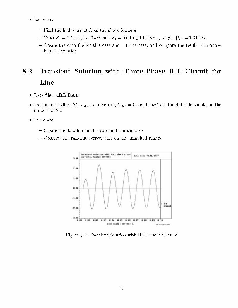
8.2 Transient Solution with Three-Phase R-L Circuit for

Line

� Data �le: 3 RL.DAT

� Except for adding �t, tmax , and setting tclose = 0 for the switch, the data �le should be thesame as in 8.1.

� Exercises:

{ Create the data �le for this case and run the case.

{ Observe the transient overvoltages on the unfaulted phases.

Figure 8.1: Transient Solution with RLC: Fault Current

30

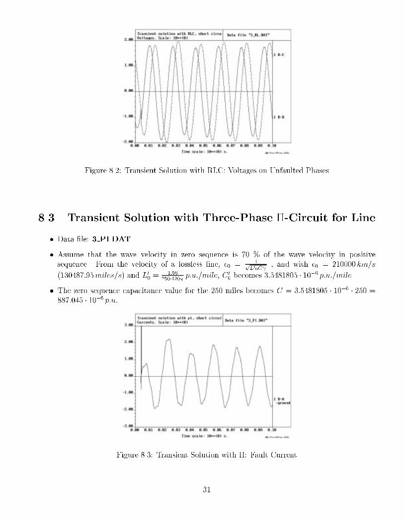
Figure 8.2: Transient Solution with RLC: Voltages on Unfaulted Phases

8.3 Transient Solution with Three-Phase �-Circuit for Line

� Data �le: 3 PI.DAT

� Assume that the wave velocity in zero sequence is 70 % of the wave velocity in positivesequence. From the velocity of a lossless line, c0 = 1p

L`0C`0, and with c0 = 210000 km=s

(130487:95miles=s) and L00 =

1:56250�120� p:u:=mile, C

00 becomes 3:5481805 � 10�6 p:u:=mile.

� The zero sequence capacitance value for the 250 miles becomes C = 3:5481805 � 10�6 � 250 =887:045 � 10�6 p:u:

Figure 8.3: Transient Solution with �: Fault Current

31

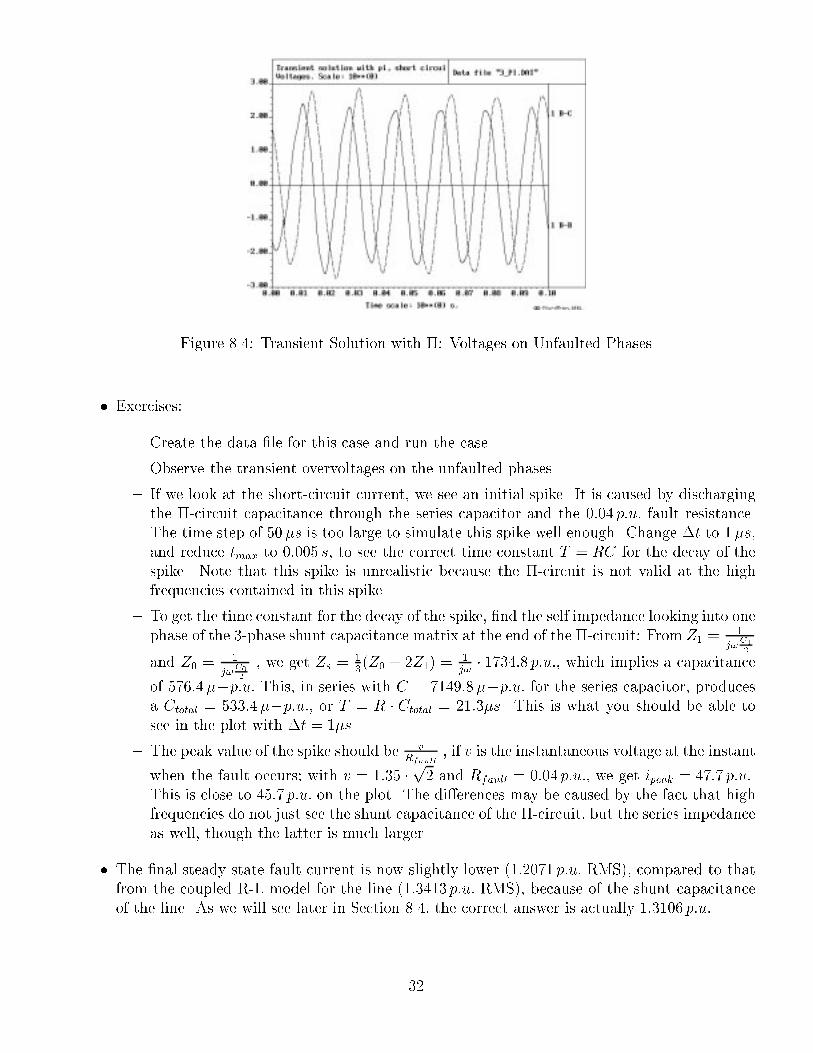
Figure 8.4: Transient Solution with �: Voltages on Unfaulted Phases

� Exercises:

{ Create the data �le for this case and run the case.

{ Observe the transient overvoltages on the unfaulted phases.

{ If we look at the short-circuit current, we see an initial spike. It is caused by dischargingthe �-circuit capacitance through the series capacitor and the 0:04 p:u: fault resistance.The time step of 50�s is too large to simulate this spike well enough. Change �t to 1�s,and reduce tmax to 0:005 s, to see the correct time constant T = RC for the decay of thespike. Note that this spike is unrealistic because the �-circuit is not valid at the highfrequencies contained in this spike.

{ To get the time constant for the decay of the spike, �nd the self impedance looking into onephase of the 3-phase shunt capacitance matrix at the end of the �-circuit: From Z1 =

1

j!C12

and Z0 =1

j!C02

, we get Zs =1

3(Z0 + 2Z1) =

1

j!� 1734:8 p:u:, which implies a capacitance

of 576:4��p:u: This, in series with C = 7149:8��p:u: for the series capacitor, producesa Ctotal = 533:4��p:u:, or T = R � Ctotal = 21:3�s. This is what you should be able tosee in the plot with �t = 1�s.

{ The peak value of the spike should be vRfault

, if v is the instantaneous voltage at the instant

when the fault occurs; with v = 1:35 � p2 and Rfault = 0:04 p:u:, we get ipeak = 47:7 p:u:.This is close to 45:7 p:u: on the plot. The di�erences may be caused by the fact that highfrequencies do not just see the shunt capacitance of the �-circuit, but the series impedanceas well, though the latter is much larger.

� The �nal steady-state fault current is now slightly lower (1:2071 p:u: RMS), compared to thatfrom the coupled R-L model for the line (1:3413 p:u: RMS), because of the shunt capacitanceof the line. As we will see later in Section 8.4, the correct answer is actually 1:3106 p:u:

32

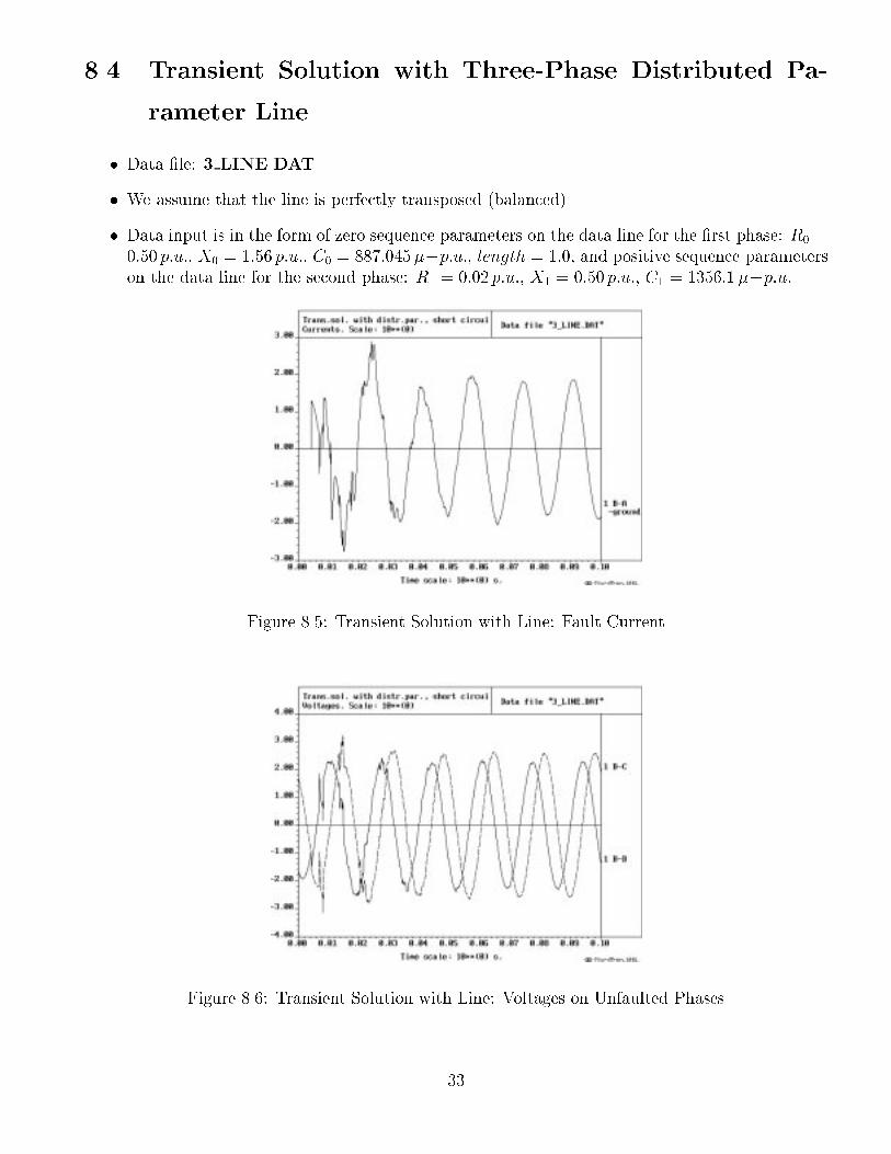
8.4 Transient Solution with Three-Phase Distributed Pa-

rameter Line

� Data �le: 3 LINE.DAT

� We assume that the line is perfectly transposed (balanced).

� Data input is in the form of zero sequence parameters on the data line for the �rst phase: R0 =0:50 p:u:, X0 = 1:56 p:u:, C0 = 887:045��p:u:, length = 1:0, and positive sequence parameterson the data line for the second phase: R1 = 0:02 p:u:, X1 = 0:50 p:u:, C1 = 1356:1��p:u:

Figure 8.5: Transient Solution with Line: Fault Current

Figure 8.6: Transient Solution with Line: Voltages on Unfaulted Phases

33

� Exercises:

{ Create the data �le for this case and run the case.

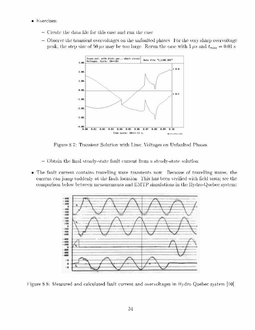
{ Observe the transient overvoltages on the unfaulted phases. For the very sharp overvoltagepeak, the step size of 50�s may be too large. Rerun the case with 1�s and tmax = 0:01 s.

Figure 8.7: Transient Solution with Line: Voltages on Unfaulted Phases

{ Obtain the �nal steady-state fault current from a steady-state solution.

� The fault current contains travelling wave transients now. Because of travelling waves, thecurrent can jump suddenly at the fault location. This has been veri�ed with �eld tests; see thecomparison below between measurements and EMTP simulations in the Hydro-Quebec system:

Figure 8.8: Measured and calculated fault current and overvoltages in Hydro-Quebec system [10]

34

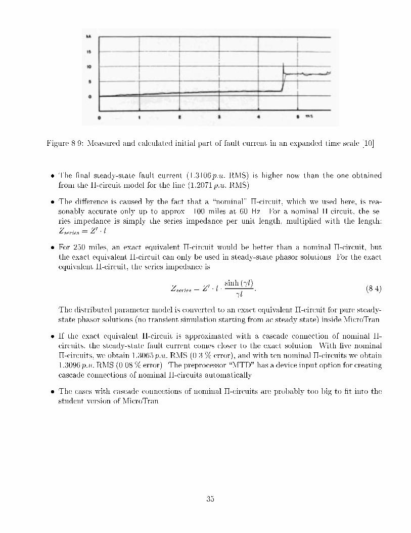
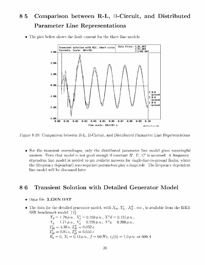
Figure 8.9: Measured and calculated initial part of fault current in an expanded time scale [10]

� The �nal steady-state fault current (1:3106 p:u: RMS) is higher now than the one obtainedfrom the �-circuit model for the line (1:2071 p:u: RMS).

� The di�erence is caused by the fact that a \nominal" �-circuit, which we used here, is rea-sonably accurate only up to approx. 100 miles at 60 Hz. For a nominal �-circuit, the se-ries impedance is simply the series impedance per unit length, multiplied with the length:Zseries = Z 0 � l.

� For 250 miles, an exact equivalent �-circuit would be better than a nominal �-circuit, butthe exact equivalent �-circuit can only be used in steady-state phasor solutions. For the exactequivalent �-circuit, the series impedance is

Zseries = Z 0 � l � sinh ( l) l

: (8.4)

The distributed parameter model is converted to an exact equivalent �-circuit for pure steady-state phasor solutions (no transient simulation starting from ac steady state) inside MicroTran.

� If the exact equivalent �-circuit is approximated with a cascade connection of nominal �-circuits, the steady-state fault current comes closer to the exact solution. With �ve nominal�-circuits, we obtain 1:3065 p:u: RMS (0.3 % error), and with ten nominal �-circuits we obtain1:3096 p:u:RMS (0.08 % error). The preprocessor \MTD" has a device input option for creatingcascade connections of nominal �-circuits automatically.

� The cases with cascade connections of nominal �-circuits are probably too big to �t into thestudent version of MicroTran.

35

8.5 Comparison between R-L, �-Circuit, and Distributed

Parameter Line Representations

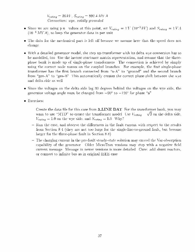
� The plot below shows the fault current for the three line models.

Figure 8.10: Comparison between R-L, �-Circuit, and Distributed Parameter Line Representations

� For the transient overvoltages, only the distributed parameter line model gives meaningfulanswers. Even that model is not good enough if constant R0, L0, C 0 is assumed. A frequency-dependent line model is needed to get realistic answers for single-line-to-ground faults, wherethe (frequency dependent) zero sequence parameters play a large role. The frequency dependentline model will be discussed later.

8.6 Transient Solution with Detailed Generator Model

� Data �le: 3 GEN.DAT

� The data for the detailed generator model, with Xd, X0d , X

00d , etc., is available from the IEEE

SSR benchmark model [11]:Xd = 1:79 p:u:, X 0

d = 0:169 p:u:, X 00d = 0:135 p:u:,Xq = 1:71 p:u:, X 0

q = 0:228 p:u:, X 00q = 0:200 p:u:,T 0d0 = 4:30 s, T 00

d0 = 0:032 sT 0q0 = 0:85 s, T 00

q0 = 0:050 sRa = 0, Xl = 0:13 p:u:, f = 60Hz, if(0) = 1:0 p:u: or 600A

36

Vrating = 26 kV , Srating = 892:4MVAConnection: wye, solidly grounded

� Since we are using p.u. values at this point, set Vrating = 1V (10�3 kV ) and Srating = 1V A(10�6MV A), to keep the generator data in per unit.

� The data for the mechanical part is left o� because we assume here that the speed does notchange.

� With a detailed generator model, the step-up transformer with its delta-wye connection has tobe modelled, too. Use the inverse reactance matrix representation, and assume that the three-phase bank is made up of single-phase transformers. The connection is achieved by simplyusing the correct node names on the coupled branches. For example, the �rst single-phasetransformer has the �rst branch connected from \a-A" to \ground" and the second branchfrom \gen-A" to \gen-B". This automatically creates the correct phase shift between the wyeand delta side as well.

� Since the voltages on the delta side lag 30 degrees behind the voltages on the wye side, thegenerator voltage angle must be changed from �90� to �120� for phase \a".

� Exercises:

{ Create the data �le for this case from 3 LINE.DAT. For the transformer bank, you maywant to use \MTD" to create the transformer model. Use Vrating =

p3 on the delta side,

Vrating = 1:0 on the wye side, and Srating = 1:0. Why?

{ Run the case, and observe the di�erences in the fault current with respect to the resultsfrom Section 8.4 (they are not too large for the single-line-to-ground fault, but becomelarger for the three-phase fault in Section 8.8).

{ The charging current in the pre-fault steady-state solution may exceed the Var-absorptioncapability of the generator. Older MicroTran versions may stop with a negative �eldcurrent message. Message in newer versions is more detailed. Cure: add shunt reactors,or connect to in�nite bus as in original IEEE case.

37

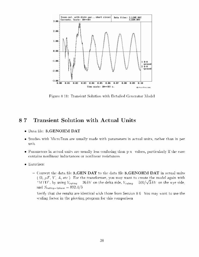
Figure 8.11: Transient Solution with Detailed Generator Model

8.7 Transient Solution with Actual Units

� Data �le: 3 GENOHM.DAT

� Studies with MicroTran are usually made with parameters in actual units, rather than in perunit.

� Parameters in actual units are usually less confusing than p.u. values, particularly if the casecontains nonlinear inductances or nonlinear resistances.

� Exercises:

{ Convert the data �le 3 GEN.DAT to the data �le 3 GENOHM.DAT in actual units( , �F , V , A, etc.). For the transformer, you may want to create the model again with\MTD", by using Vrating = 26 kV on the delta side, Vrating = 500=

p3 kV on the wye side,

and Srating�1phase = 892:4=3.

{ Verify that the results are identical with those from Section 8.6. You may want to use thescaling factor in the plotting program for this comparison.

38

8.8 Transient Solution for Simultaneous Three-Phase

Short-Circuit

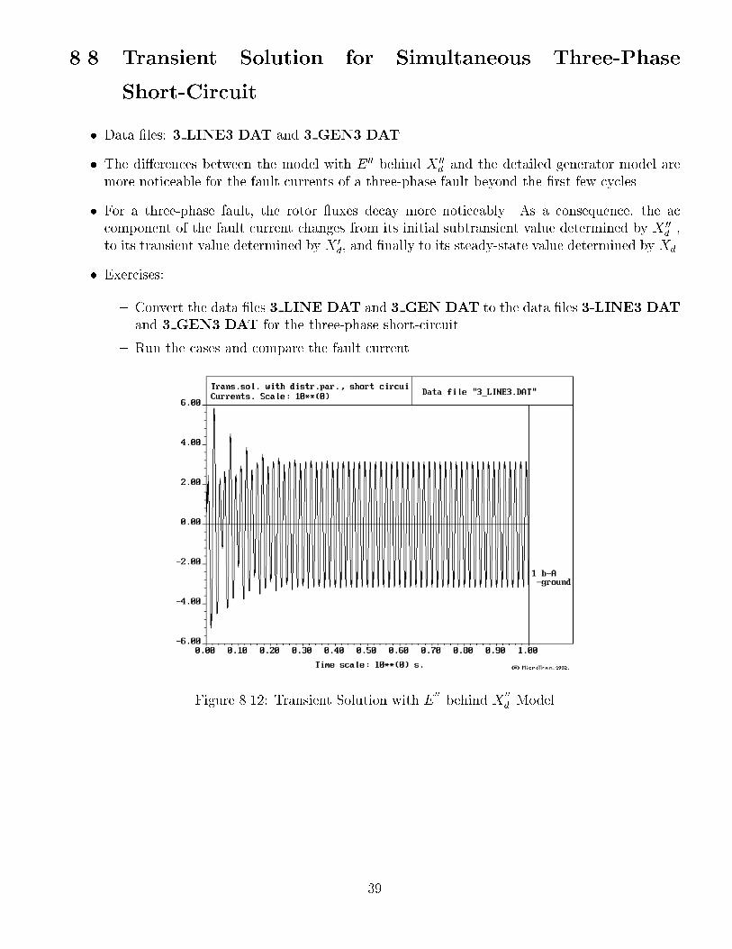
� Data �les: 3 LINE3.DAT and 3 GEN3.DAT

� The di�erences between the model with E 00 behind X 00d and the detailed generator model are

more noticeable for the fault currents of a three-phase fault beyond the �rst few cycles.

� For a three-phase fault, the rotor uxes decay more noticeably. As a consequence, the accomponent of the fault current changes from its initial subtransient value determined by X 00

d ,to its transient value determined by X 0

d, and �nally to its steady-state value determined by Xd.

� Exercises:

{ Convert the data �les 3 LINE.DAT and 3 GEN.DAT to the data �les 3-LINE3.DATand 3 GEN3.DAT for the three-phase short-circuit.

{ Run the cases and compare the fault current.

Figure 8.12: Transient Solution with E00

behind X00

d Model

39

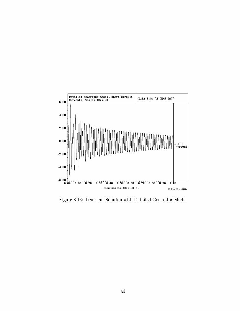
Figure 8.13: Transient Solution with Detailed Generator Model

40

8.9 Short-Circuits on HVDC Lines

� Short-circuit currents on HVDC lines, and related transient overvoltages, can only be calculatedwith EMTP-type programs.

Figure 8.14: Measured and calculated transient overvoltage on unfaulted pole of HVDC line [12]

41

Appendix A

Relationship between Phase Quantities

and Sequence Quantities

Assume that a three-phase transmission line is represented with series R-L branches. For steady-statesolutions, the voltage drop along the three phases would then be

264�Va�Vb�Vc

375 =

264Zs Zm Zm

Zm Zs Zm

Zm Zm Zs

375 �

264IaIbIc

375 (A.1)

where Zs is the self impedance of each phase (with ground and ground wires providing the returnpath), and Zm is the mutual impedance between phases. In Equation (A.1), we assume that thetransmission line is \balanced" (perfectly transposed). Otherwise, the matrix would be

264Zaa Zab Zac

Zba Zbb Zbc

Zca Zcb Zcc

375 (A.2)

(still symmetric, Zba = Zab, etc.).

Equations A.1 with phase quantities are coupled. They become simpler, namely decoupled, if wework with \symmetrical components", by transforming phase quantities Ia, Ib, Ic to \sequence"quantities Izero, Ipositive, Inegative:

264

�Vzero�Vpositive�Vnegative

375 =

264Zzero 0 00 Zpositive 00 0 Znegative

375 �

264

IzeroIpositiveInegative

375 (A.3)

Since the matrix is diagonal, we can solve the equations separately for zero, positive, and negativesequence quantities, as if we had three single-phase networks rather than one three-phase network.This is a transformation based on eigenvalues and eigenvectors. The transformations are

42

264

IzeroIpositiveInegative

375 =

1p3

2641 1 11 a a2

1 a2 a

375 �

264IaIbIc

375 ; (A.4)

and 264IaIbIc

375 =

1p3

2641 1 11 a2 a1 a a2

375 �

264

IzeroIpositiveInegative

375 (A.5)

where a = ej120�

, a2 = e�j120�

. The transformations for voltages are identical. Above transformationsare \normalized". If unnormalized (usual practice in power industry), the factor in Equation (A.4)is 1

3, and in (A.5) it is 1.

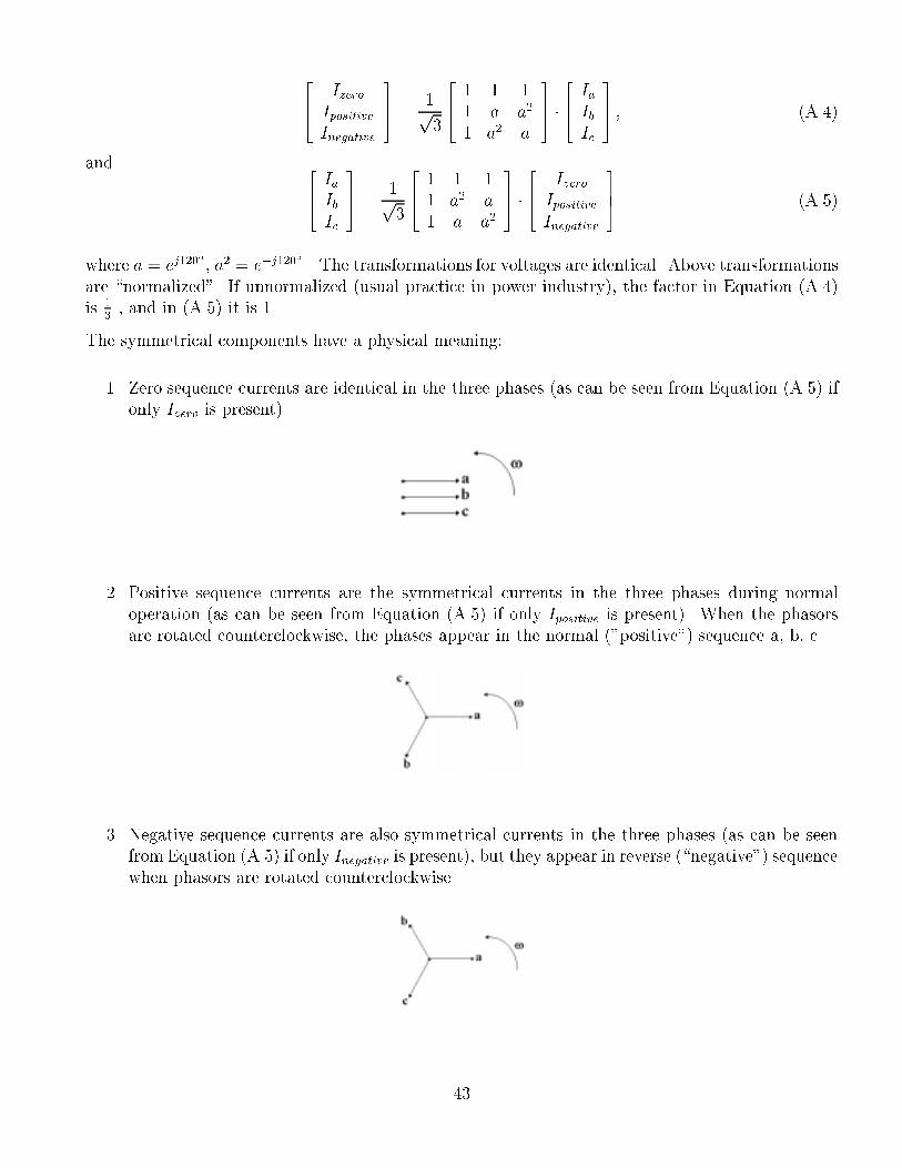
The symmetrical components have a physical meaning:

1. Zero sequence currents are identical in the three phases (as can be seen from Equation (A.5) ifonly Izero is present).

2. Positive sequence currents are the symmetrical currents in the three phases during normaloperation (as can be seen from Equation (A.5) if only Ipositive is present). When the phasorsare rotated counterclockwise, the phases appear in the normal ("positive") sequence a, b, c.

3. Negative sequence currents are also symmetrical currents in the three phases (as can be seenfrom Equation (A.5) if only Inegative is present), but they appear in reverse (\negative") sequencewhen phasors are rotated counterclockwise.

43

Approach in MicroTran:

� Symmetrical component equations make no sense for untransposed lines, because the trans-formed matrix in sequence quantities is no longer diagonal.

� All network components must be three phase with symmetrical component equations. If asingle-phase distribution line (one phase conductor and one neutral conductor) were connectedto a three-phase substation, that would be di�cult to model with symmetrical components.

� For reasons of generality, MicroTran therefore works with phase quantities, even when inputdata is given in sequence quantities.

� The zero sequence impedance can be obtained from Equation (A.1). With all voltages equal,we need only the �rst equation for �Va, and with Ib = Ia, Ic = Ia, we get

�Va = (Zs + 2Zm) � Ia (A.6)

The zero sequence impedance (subscript \zero" or \0") is therefore:

Z0 = Zs + 2Zm (A.7)

� For the positive sequence impedance, we use in Equation (A.1) Ib = a2Ia, Ic = aIa , and weget

�Va = (Zs � Zm) � Ia (A.8)

The positive sequence impedance (subscript \positive" or \1") is therefore:

Z1 = Zs � Zm (A.9)

� Similarly, the negative sequence impedance (subscript \negative" or \2") becomes

Z2 = Zs � Zm (A.10)

44

Bibliography

[1] M. B. Hughes, R. W. Leonard, and T. G. Martinich, \Measurement of power system sub-synchronous driving point impedance and comparison with computer simulations," IEEETransactions on Power Apparatus and Systems, vol. PAS-103, pp. 619 - 630, March 1984.

[2] C. A. F. Cunha and H. W. Dommel, \Computer simulation of �eld tests on the 345 kV Jaguara-Taquaril line," Paper BH/GSP/12 (in Portuguese), in II Semin�ario Nacional de Produ�c~ao eTransmissao de Energia El�etrica, Belo Horizonte, Brazil, 1973.

[3] J. R. Mart��, \Accurate modelling of frequency-dependent transmission lines in electromagnetictransient simulations," IEEE Transactions on Power Apparatus and Systems, vol. PAS-101,pp. 147 - 157, Jan. 1982.

[4] M. Rioual, \Measurements and computer simulation of fast transients through indoor andoutdoor substations," IEEE Transactions on Power Delivery, vol. 5, pp. 117 - 123, Jan. 1990.

[5] H.W. Dommel, Case Studies for Electromagnetic Transients, 2nd Edition, Microtran PowerSystem Analysis Corporation, Vancouver, British Columbia, Canada, 1993.

[6] D. H. Baker, \Synchronous machine modeling in EMTP," IEEE Course Text: Digital Sim-ulation of Electrical Transient Phenomena, No. 81 EHO173-5-PWR, IEEE Service Center,Piscataway, N.J., 1980.

[7] Transformer Inrush Current, Test Case 1., Microtran Power System Analysis Corporation,Vancouver, British Columbia, Canada, 1990.

[8] A. C. S. de Lima, personal communication, July 1998.

[9] W. Xu, J. R. Mart��, and H. W. Dommel, \A multiphase harmonic load ow solution technique,"IEEE Transactions on Power Systems, vol. 6, pp. 174 - 190, Febr. 1991.

[10] R. Malewski, V. N. Narancic, and Y. Robichaud, \Behavior of the Hydro-Quebec 735-kVsystem under transient short-circuit conditions and its digital computer simulation," IEEETransactions on Power Apparatus and Systems, vol. PAS-94, pp. 425 - 431, March/April 1975.

[11] IEEE Task Force, \First benchmark model for computer simulation of subsynchronous reso-nance," IEEE Transactions on Power Apparatus and Systems, vol. PAS-96, pp. 1565 - 1572,Sept./Oct. 1977.

45

[12] D. J. Melvold, P. C. Odam, and J. J. Vithayathil, \Transient overvoltages on an HVDC bipolarline during monopolar line faults," IEEE Transactions on Power Apparatus and Systems, PAS-96, pp. 591 - 601, March/April 1977.

46