Embed Size (px)
Citation preview
============================================================Dependent Variable: LGHOUS Method: Least Squares Sample: 1959 2003 Included observations: 45 ============================================================ Variable Coefficient Std. Error t-Statistic Prob. ============================================================ C 0.005625 0.167903 0.033501 0.9734 LGDPI 1.031918 0.006649 155.1976 0.0000 LGPRHOUS -0.483421 0.041780 -11.57056 0.0000============================================================R-squared 0.998583 Mean dependent var 6.359334Adjusted R-squared 0.998515 S.D. dependent var 0.437527S.E. of regression 0.016859 Akaike info criter-5.263574Sum squared resid 0.011937 Schwarz criterion -5.143130Log likelihood 121.4304 F-statistic 14797.05Durbin-Watson stat 0.633113 Prob(F-statistic) 0.000000============================================================
1
HOUSING DYNAMICS
This sequence gives an example of how a direct examination of plots of the residuals and the data for the variables in a regression model may lead to an improvement in the specification of the regression model.
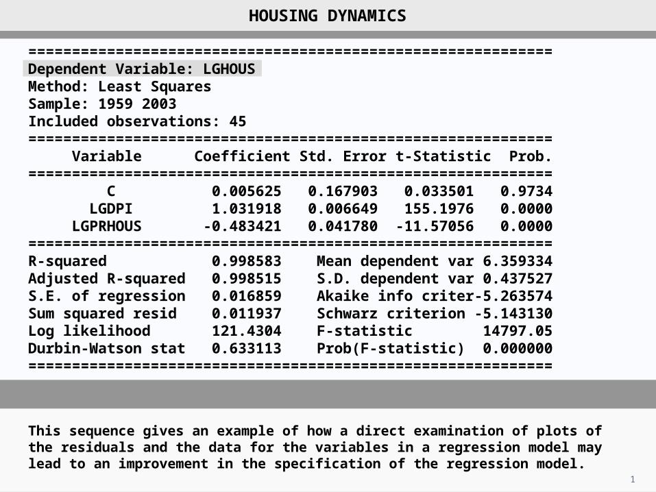
============================================================Dependent Variable: LGHOUS Method: Least Squares Sample: 1959 2003 Included observations: 45 ============================================================ Variable Coefficient Std. Error t-Statistic Prob. ============================================================ C 0.005625 0.167903 0.033501 0.9734 LGDPI 1.031918 0.006649 155.1976 0.0000 LGPRHOUS -0.483421 0.041780 -11.57056 0.0000============================================================R-squared 0.998583 Mean dependent var 6.359334Adjusted R-squared 0.998515 S.D. dependent var 0.437527S.E. of regression 0.016859 Akaike info criter-5.263574Sum squared resid 0.011937 Schwarz criterion -5.143130Log likelihood 121.4304 F-statistic 14797.05Durbin-Watson stat 0.633113 Prob(F-statistic) 0.000000============================================================
2
The regression output is that for a logarithmic regression of aggregate expenditure on housing services on income and relative price for the United States for the period 1959–2003. The income and price elasticities seem plausible.
HOUSING DYNAMICS
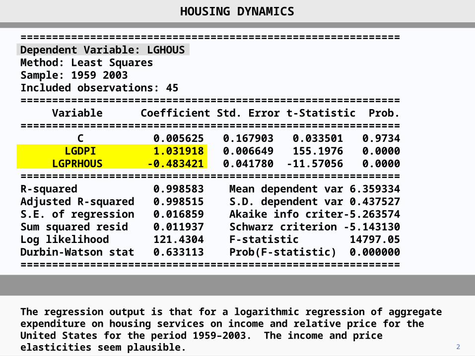
============================================================Dependent Variable: LGHOUS Method: Least Squares Sample: 1959 2003 Included observations: 45 ============================================================ Variable Coefficient Std. Error t-Statistic Prob. ============================================================ C 0.005625 0.167903 0.033501 0.9734 LGDPI 1.031918 0.006649 155.1976 0.0000 LGPRHOUS -0.483421 0.041780 -11.57056 0.0000============================================================R-squared 0.998583 Mean dependent var 6.359334Adjusted R-squared 0.998515 S.D. dependent var 0.437527S.E. of regression 0.016859 Akaike info criter-5.263574Sum squared resid 0.011937 Schwarz criterion -5.143130Log likelihood 121.4304 F-statistic 14797.05Durbin-Watson stat 0.633113 Prob(F-statistic) 0.000000============================================================
3
However, the Breusch–Godfrey and Durbin–Watson statistics both indicate autocorrelation at a high significance level.
Breusch–Godfrey statistic: 20.02
c2(1)crit, 0.1% = 10.83
HOUSING DYNAMICS
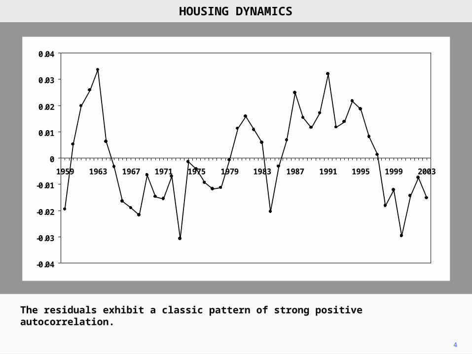
4
The residuals exhibit a classic pattern of strong positive autocorrelation.
-0.04
-0.03
-0.02
-0.01
0
0.01
0.02
0.03
0.04
1959 1963 1967 1971 1975 1979 1983 1987 1991 1995 1999 2003
HOUSING DYNAMICS
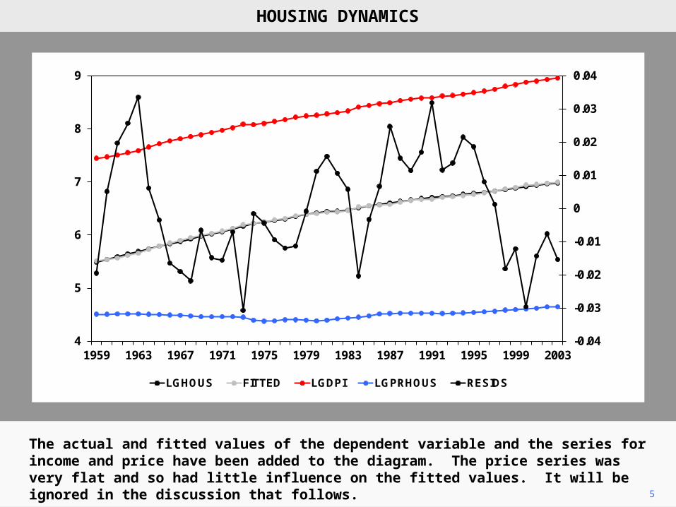
5
The actual and fitted values of the dependent variable and the series for income and price have been added to the diagram. The price series was very flat and so had little influence on the fitted values. It will be ignored in the discussion that follows.
HOUSING DYNAMICS
-0.04
-0.03
-0.02
-0.01
0
0.01
0.02
0.03
0.04
4
5
6
7
8
9
1959 1963 1967 1971 1975 1979 1983 1987 1991 1995 1999 2003
LGHOUS FITTED LGDPI LGPRHOUS RESIDS
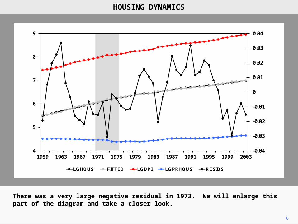
6
There was a very large negative residual in 1973. We will enlarge this part of the diagram and take a closer look.
HOUSING DYNAMICS
-0.04
-0.03
-0.02
-0.01
0
0.01
0.02
0.03
0.04
4
5
6
7
8
9
1959 1963 1967 1971 1975 1979 1983 1987 1991 1995 1999 2003
LGHOUS FITTED LGDPI LGPRHOUS RESIDS
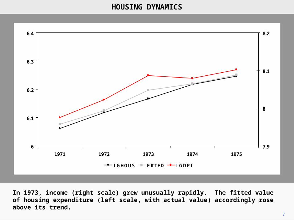
7
In 1973, income (right scale) grew unusually rapidly. The fitted value of housing expenditure (left scale, with actual value) accordingly rose above its trend.
6
6.1
6.2
6.3
6.4
1971 1972 1973 1974 1975
7.9
8
8.1
8.2
LGHOUS FITTED LGDPI
HOUSING DYNAMICS
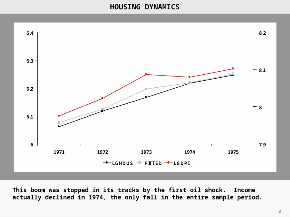
8
This boom was stopped in its tracks by the first oil shock. Income actually declined in 1974, the only fall in the entire sample period.
HOUSING DYNAMICS
6
6.1
6.2
6.3
6.4
1971 1972 1973 1974 1975
7.9
8
8.1
8.2
LGHOUS FITTED LGDPI
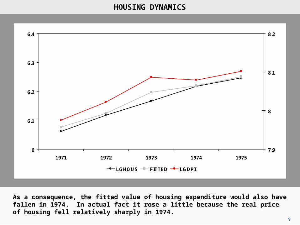
9
As a consequence, the fitted value of housing expenditure would also have fallen in 1974. In actual fact it rose a little because the real price of housing fell relatively sharply in 1974.
HOUSING DYNAMICS
6
6.1
6.2
6.3
6.4
1971 1972 1973 1974 1975
7.9
8
8.1
8.2
LGHOUS FITTED LGDPI
10
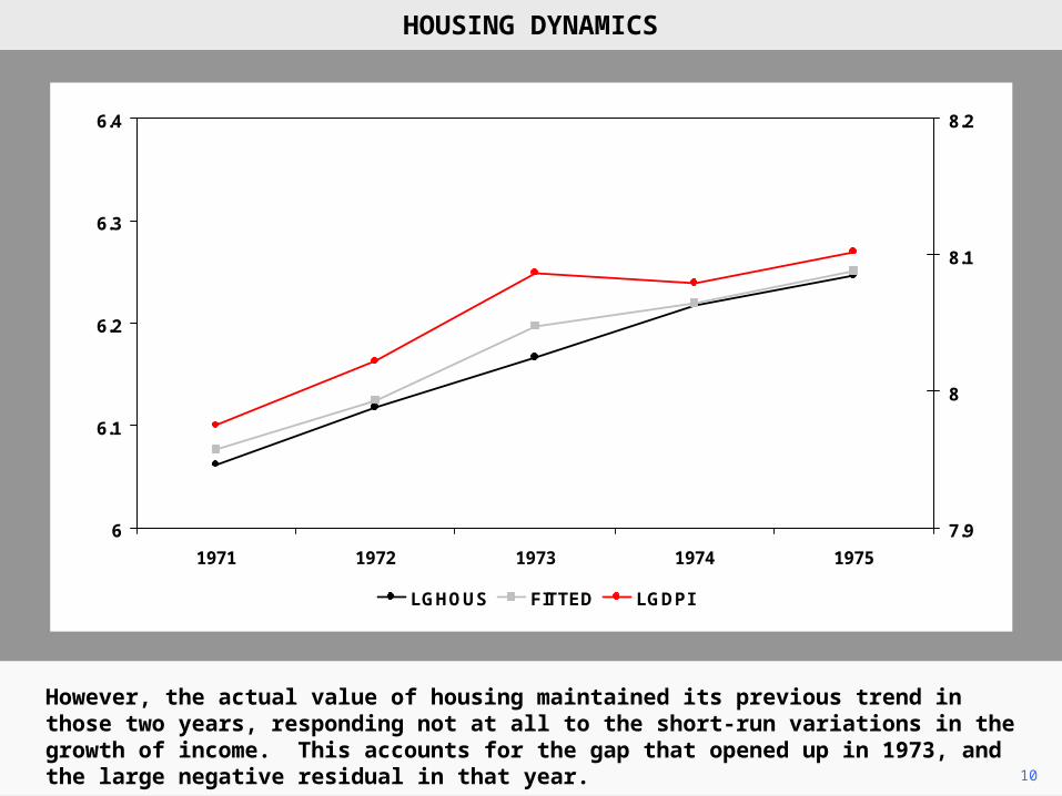
However, the actual value of housing maintained its previous trend in those two years, responding not at all to the short-run variations in the growth of income. This accounts for the gap that opened up in 1973, and the large negative residual in that year.
HOUSING DYNAMICS
6
6.1
6.2
6.3
6.4
1971 1972 1973 1974 1975
7.9
8
8.1
8.2
LGHOUS FITTED LGDPI
11
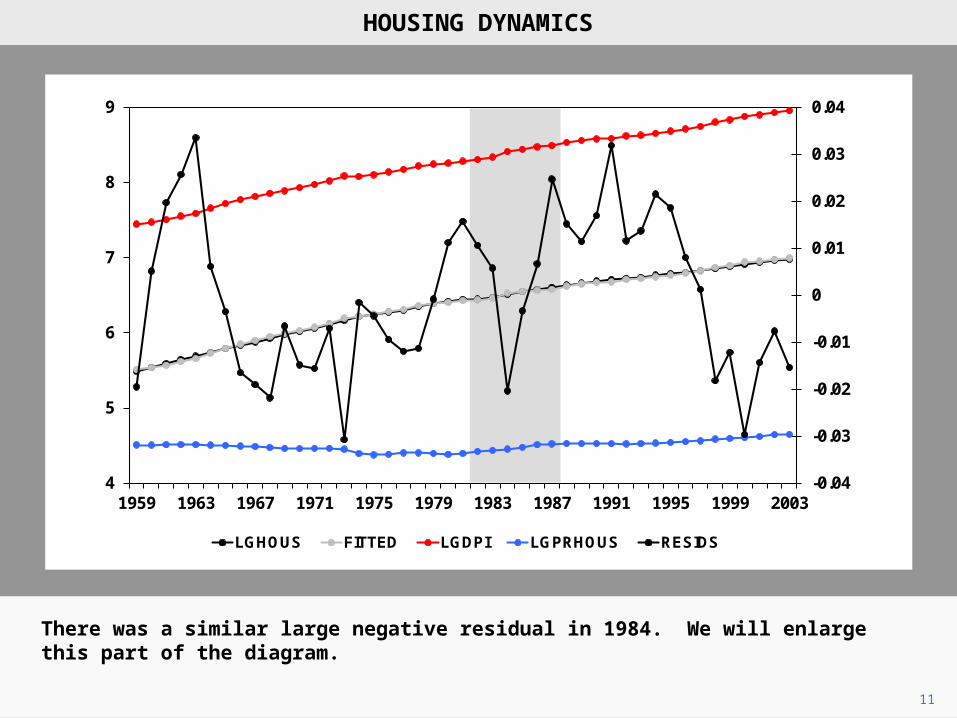
There was a similar large negative residual in 1984. We will enlarge this part of the diagram.
HOUSING DYNAMICS
-0.04
-0.03
-0.02
-0.01
0
0.01
0.02
0.03
0.04
4
5
6
7
8
9
1959 1963 1967 1971 1975 1979 1983 1987 1991 1995 1999 2003
LGHOUS FITTED LGDPI LGPRHOUS RESIDS
6.4
6.5
6.6
1982 1983 1984 1985 1986 1987
8.2
8.3
8.4
8.5
LGHOUS FITTED LGDPI
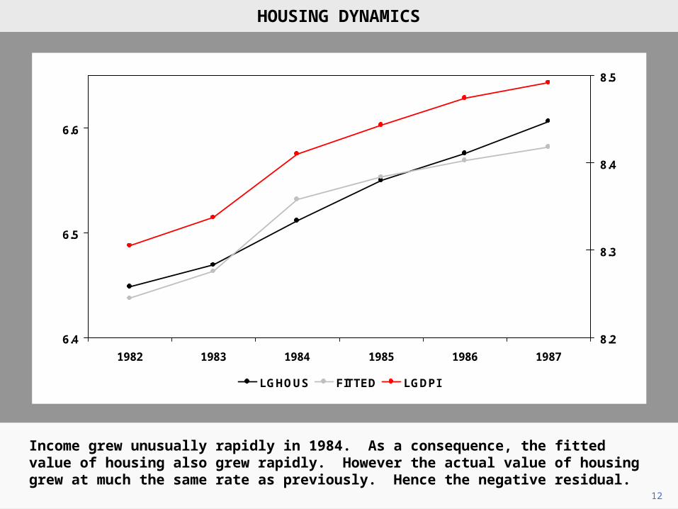
12
Income grew unusually rapidly in 1984. As a consequence, the fitted value of housing also grew rapidly. However the actual value of housing grew at much the same rate as previously. Hence the negative residual.
HOUSING DYNAMICS
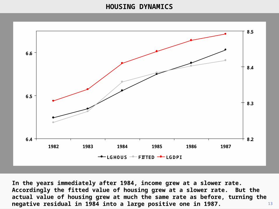
13
In the years immediately after 1984, income grew at a slower rate. Accordingly the fitted value of housing grew at a slower rate. But the actual value of housing grew at much the same rate as before, turning the negative residual in 1984 into a large positive one in 1987.
HOUSING DYNAMICS
6.4
6.5
6.6
1982 1983 1984 1985 1986 1987
8.2
8.3
8.4
8.5
LGHOUS FITTED LGDPI
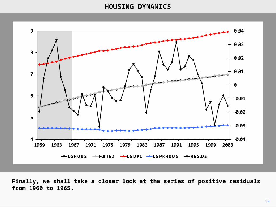
14
Finally, we shall take a closer look at the series of positive residuals from 1960 to 1965.
HOUSING DYNAMICS
-0.04
-0.03
-0.02
-0.01
0
0.01
0.02
0.03
0.04
4
5
6
7
8
9
1959 1963 1967 1971 1975 1979 1983 1987 1991 1995 1999 2003
LGHOUS FITTED LGDPI LGPRHOUS RESIDS
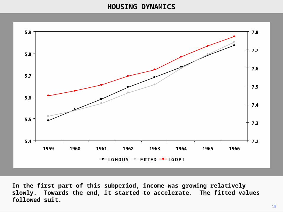
15
In the first part of this subperiod, income was growing relatively slowly. Towards the end, it started to accelerate. The fitted values followed suit.
5.4
5.5
5.6
5.7
5.8
5.9
1959 1960 1961 1962 1963 1964 1965 1966
7.2
7.3
7.4
7.5
7.6
7.7
7.8
LGHOUS FITTED LGDPI
HOUSING DYNAMICS
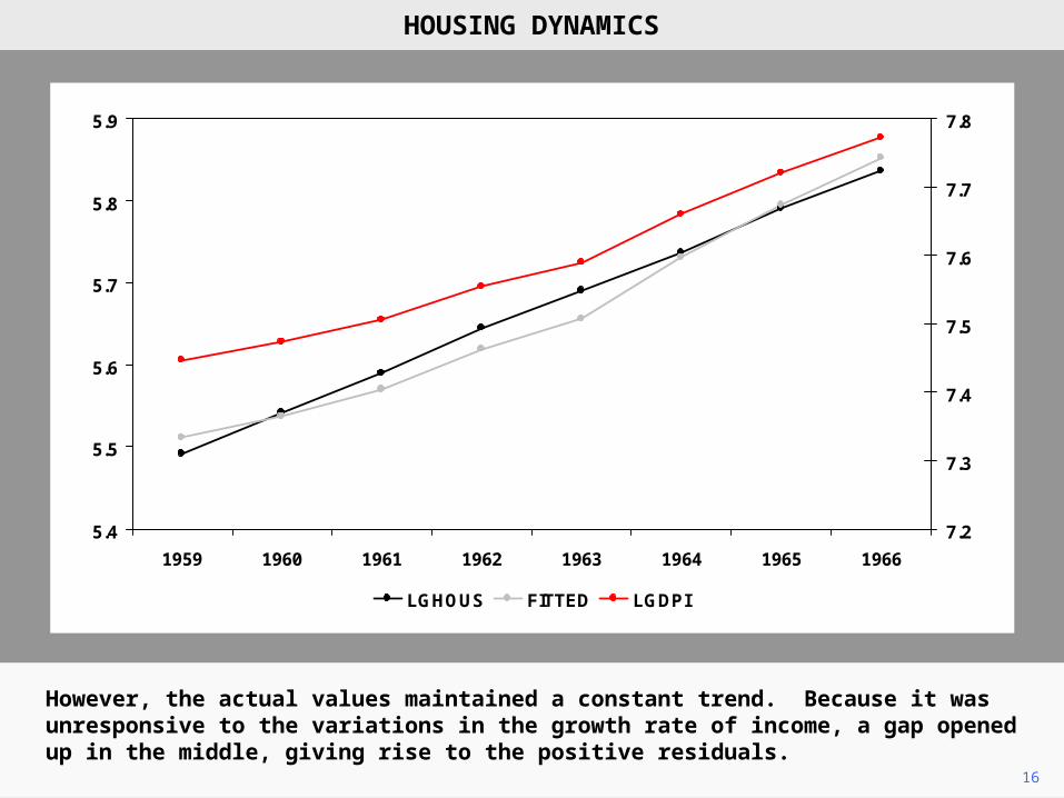
16
However, the actual values maintained a constant trend. Because it was unresponsive to the variations in the growth rate of income, a gap opened up in the middle, giving rise to the positive residuals.
HOUSING DYNAMICS
5.4
5.5
5.6
5.7
5.8
5.9
1959 1960 1961 1962 1963 1964 1965 1966
7.2
7.3
7.4
7.5
7.6
7.7
7.8
LGHOUS FITTED LGDPI
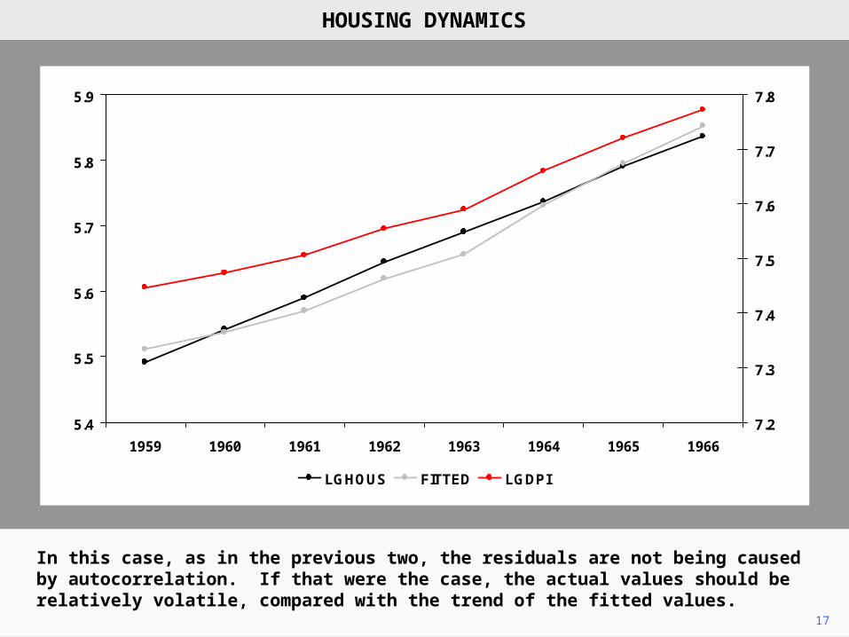
17
In this case, as in the previous two, the residuals are not being caused by autocorrelation. If that were the case, the actual values should be relatively volatile, compared with the trend of the fitted values.
HOUSING DYNAMICS
5.4
5.5
5.6
5.7
5.8
5.9
1959 1960 1961 1962 1963 1964 1965 1966
7.2
7.3
7.4
7.5
7.6
7.7
7.8
LGHOUS FITTED LGDPI
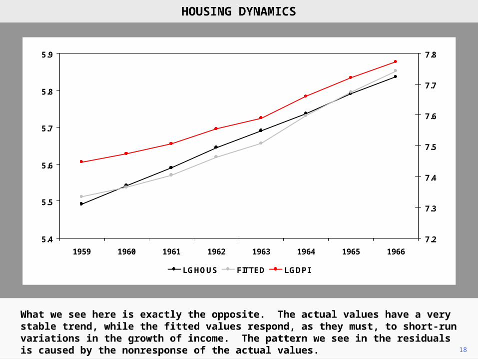
18
What we see here is exactly the opposite. The actual values have a very stable trend, while the fitted values respond, as they must, to short-run variations in the growth of income. The pattern we see in the residuals is caused by the nonresponse of the actual values.
HOUSING DYNAMICS
5.4
5.5
5.6
5.7
5.8
5.9
1959 1960 1961 1962 1963 1964 1965 1966
7.2
7.3
7.4
7.5
7.6
7.7
7.8
LGHOUS FITTED LGDPI
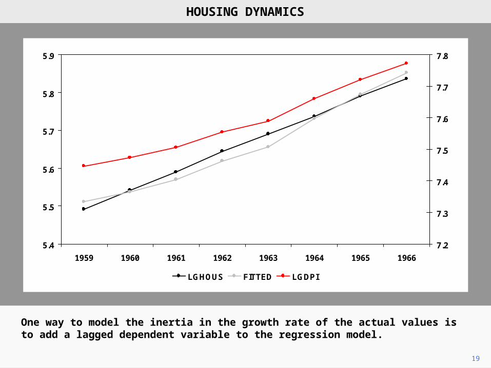
19
One way to model the inertia in the growth rate of the actual values is to add a lagged dependent variable to the regression model.
HOUSING DYNAMICS
5.4
5.5
5.6
5.7
5.8
5.9
1959 1960 1961 1962 1963 1964 1965 1966
7.2
7.3
7.4
7.5
7.6
7.7
7.8
LGHOUS FITTED LGDPI
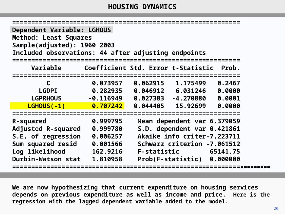
20
We are now hypothesizing that current expenditure on housing services depends on previous expenditure as well as income and price. Here is the regression with the lagged dependent variable added to the model.
HOUSING DYNAMICS
============================================================Dependent Variable: LGHOUS Method: Least Squares Sample(adjusted): 1960 2003 Included observations: 44 after adjusting endpoints ============================================================ Variable Coefficient Std. Error t-Statistic Prob. ============================================================ C 0.073957 0.062915 1.175499 0.2467 LGDPI 0.282935 0.046912 6.031246 0.0000 LGPRHOUS -0.116949 0.027383 -4.270880 0.0001 LGHOUS(-1) 0.707242 0.044405 15.92699 0.0000============================================================R-squared 0.999795 Mean dependent var 6.379059Adjusted R-squared 0.999780 S.D. dependent var 0.421861S.E. of regression 0.006257 Akaike info criter-7.223711Sum squared resid 0.001566 Schwarz criterion -7.061512Log likelihood 162.9216 F-statistic 65141.75Durbin-Watson stat 1.810958 Prob(F-statistic) 0.000000=====================================================================
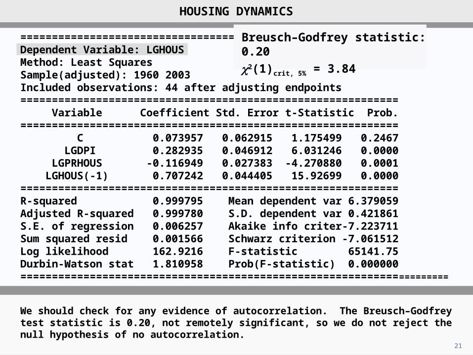
21
We should check for any evidence of autocorrelation. The Breusch–Godfrey test statistic is 0.20, not remotely significant, so we do not reject the null hypothesis of no autocorrelation.
HOUSING DYNAMICS
============================================================Dependent Variable: LGHOUS Method: Least Squares Sample(adjusted): 1960 2003 Included observations: 44 after adjusting endpoints ============================================================ Variable Coefficient Std. Error t-Statistic Prob. ============================================================ C 0.073957 0.062915 1.175499 0.2467 LGDPI 0.282935 0.046912 6.031246 0.0000 LGPRHOUS -0.116949 0.027383 -4.270880 0.0001 LGHOUS(-1) 0.707242 0.044405 15.92699 0.0000============================================================R-squared 0.999795 Mean dependent var 6.379059Adjusted R-squared 0.999780 S.D. dependent var 0.421861S.E. of regression 0.006257 Akaike info criter-7.223711Sum squared resid 0.001566 Schwarz criterion -7.061512Log likelihood 162.9216 F-statistic 65141.75Durbin-Watson stat 1.810958 Prob(F-statistic) 0.000000=====================================================================
Breusch–Godfrey statistic: 0.20
c2(1)crit, 5% = 3.84
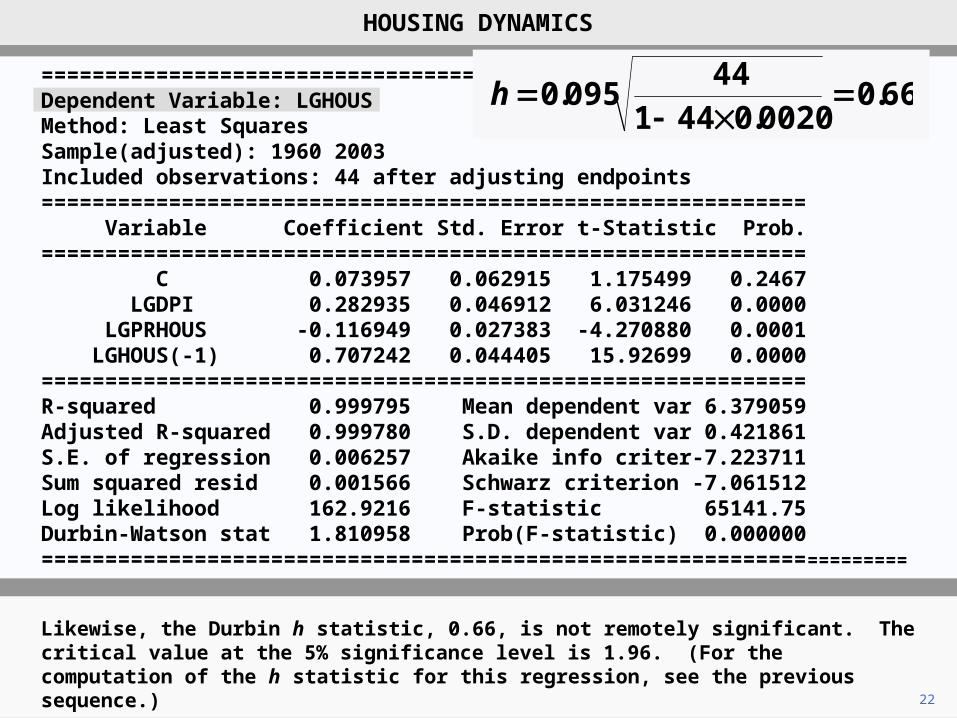
22
Likewise, the Durbin h statistic, 0.66, is not remotely significant. The critical value at the 5% significance level is 1.96. (For the computation of the h statistic for this regression, see the previous sequence.)
HOUSING DYNAMICS
============================================================Dependent Variable: LGHOUS Method: Least Squares Sample(adjusted): 1960 2003 Included observations: 44 after adjusting endpoints ============================================================ Variable Coefficient Std. Error t-Statistic Prob. ============================================================ C 0.073957 0.062915 1.175499 0.2467 LGDPI 0.282935 0.046912 6.031246 0.0000 LGPRHOUS -0.116949 0.027383 -4.270880 0.0001 LGHOUS(-1) 0.707242 0.044405 15.92699 0.0000============================================================R-squared 0.999795 Mean dependent var 6.379059Adjusted R-squared 0.999780 S.D. dependent var 0.421861S.E. of regression 0.006257 Akaike info criter-7.223711Sum squared resid 0.001566 Schwarz criterion -7.061512Log likelihood 162.9216 F-statistic 65141.75Durbin-Watson stat 1.810958 Prob(F-statistic) 0.000000=====================================================================
66.00020.0441
44095.0
h
23
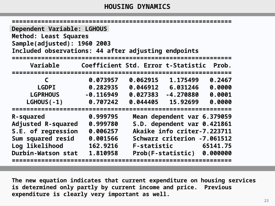
The new equation indicates that current expenditure on housing services is determined only partly by current income and price. Previous expenditure is clearly very important as well.
HOUSING DYNAMICS
============================================================Dependent Variable: LGHOUS Method: Least Squares Sample(adjusted): 1960 2003 Included observations: 44 after adjusting endpoints ============================================================ Variable Coefficient Std. Error t-Statistic Prob. ============================================================ C 0.073957 0.062915 1.175499 0.2467 LGDPI 0.282935 0.046912 6.031246 0.0000 LGPRHOUS -0.116949 0.027383 -4.270880 0.0001 LGHOUS(-1) 0.707242 0.044405 15.92699 0.0000============================================================R-squared 0.999795 Mean dependent var 6.379059Adjusted R-squared 0.999780 S.D. dependent var 0.421861S.E. of regression 0.006257 Akaike info criter-7.223711Sum squared resid 0.001566 Schwarz criterion -7.061512Log likelihood 162.9216 F-statistic 65141.75Durbin-Watson stat 1.810958 Prob(F-statistic) 0.000000============================================================
24
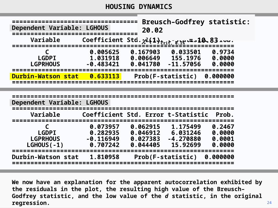
We now have an explanation for the apparent autocorrelation exhibited by the residuals in the plot, the resulting high value of the Breusch–Godfrey statistic, and the low value of the d statistic, in the original regression.
HOUSING DYNAMICS
============================================================Dependent Variable: LGHOUS ============================================================ Variable Coefficient Std. Error t-Statistic Prob. ============================================================ C 0.005625 0.167903 0.033501 0.9734 LGDPI 1.031918 0.006649 155.1976 0.0000 LGPRHOUS -0.483421 0.041780 -11.57056 0.0000============================================================Durbin-Watson stat 0.633113 Prob(F-statistic) 0.000000============================================================
============================================================Dependent Variable: LGHOUS ============================================================ Variable Coefficient Std. Error t-Statistic Prob. ============================================================ C 0.073957 0.062915 1.175499 0.2467 LGDPI 0.282935 0.046912 6.031246 0.0000 LGPRHOUS -0.116949 0.027383 -4.270880 0.0001 LGHOUS(-1) 0.707242 0.044405 15.92699 0.0000============================================================Durbin-Watson stat 1.810958 Prob(F-statistic) 0.000000============================================================
Breusch–Godfrey statistic: 20.02
c2(1)crit, 0.1% = 10.83
24
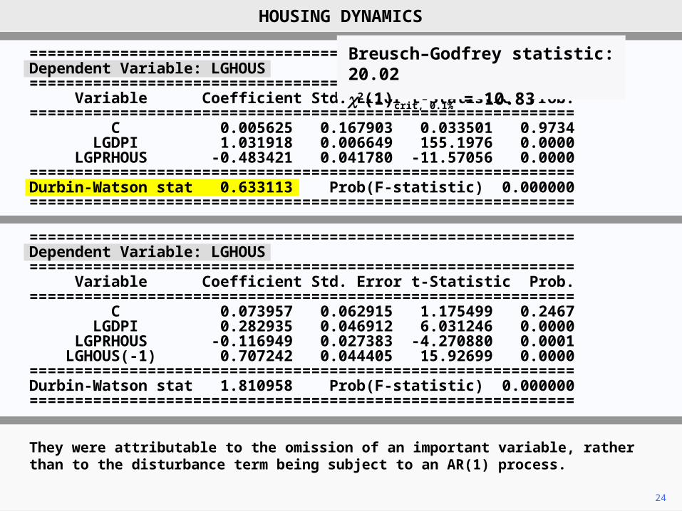
They were attributable to the omission of an important variable, rather than to the disturbance term being subject to an AR(1) process.
HOUSING DYNAMICS
============================================================Dependent Variable: LGHOUS ============================================================ Variable Coefficient Std. Error t-Statistic Prob. ============================================================ C 0.005625 0.167903 0.033501 0.9734 LGDPI 1.031918 0.006649 155.1976 0.0000 LGPRHOUS -0.483421 0.041780 -11.57056 0.0000============================================================Durbin-Watson stat 0.633113 Prob(F-statistic) 0.000000============================================================
============================================================Dependent Variable: LGHOUS ============================================================ Variable Coefficient Std. Error t-Statistic Prob. ============================================================ C 0.073957 0.062915 1.175499 0.2467 LGDPI 0.282935 0.046912 6.031246 0.0000 LGPRHOUS -0.116949 0.027383 -4.270880 0.0001 LGHOUS(-1) 0.707242 0.044405 15.92699 0.0000============================================================Durbin-Watson stat 1.810958 Prob(F-statistic) 0.000000============================================================
Breusch–Godfrey statistic: 20.02
c2(1)crit, 0.1% = 10.83
25
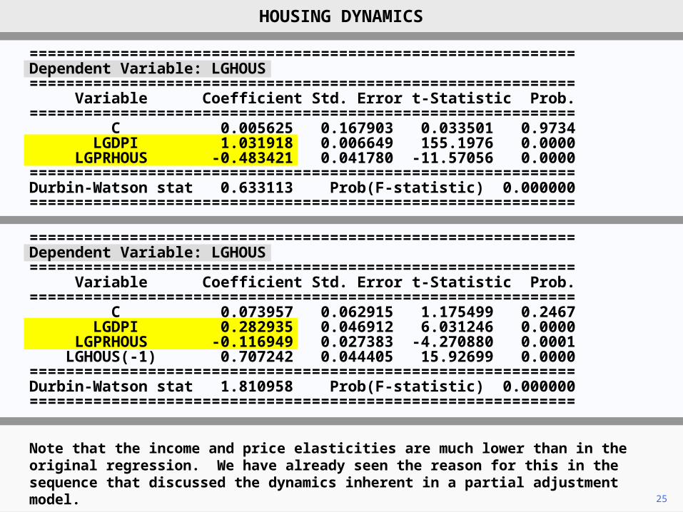
Note that the income and price elasticities are much lower than in the original regression. We have already seen the reason for this in the sequence that discussed the dynamics inherent in a partial adjustment model.
HOUSING DYNAMICS
============================================================Dependent Variable: LGHOUS ============================================================ Variable Coefficient Std. Error t-Statistic Prob. ============================================================ C 0.005625 0.167903 0.033501 0.9734 LGDPI 1.031918 0.006649 155.1976 0.0000 LGPRHOUS -0.483421 0.041780 -11.57056 0.0000============================================================Durbin-Watson stat 0.633113 Prob(F-statistic) 0.000000============================================================
============================================================Dependent Variable: LGHOUS ============================================================ Variable Coefficient Std. Error t-Statistic Prob. ============================================================ C 0.073957 0.062915 1.175499 0.2467 LGDPI 0.282935 0.046912 6.031246 0.0000 LGPRHOUS -0.116949 0.027383 -4.270880 0.0001 LGHOUS(-1) 0.707242 0.044405 15.92699 0.0000============================================================Durbin-Watson stat 1.810958 Prob(F-statistic) 0.000000============================================================

Copyright Christopher Dougherty 2013.
These slideshows may be downloaded by anyone, anywhere for personal use.
Subject to respect for copyright and, where appropriate, attribution, they may be
used as a resource for teaching an econometrics course. There is no need to
refer to the author.
The content of this slideshow comes from Section 12.4 of C. Dougherty,
Introduction to Econometrics, fourth edition 2011, Oxford University Press.
Additional (free) resources for both students and instructors may be
downloaded from the OUP Online Resource Centre
http://www.oup.com/uk/orc/bin/9780199567089/.
Individuals studying econometrics on their own who feel that they might benefit
from participation in a formal course should consider the London School of
Economics summer school course
EC212 Introduction to Econometrics
http://www2.lse.ac.uk/study/summerSchools/summerSchool/Home.aspx
or the University of London International Programmes distance learning course
EC2020 Elements of Econometrics
www.londoninternational.ac.uk/lse.
2013.03.04