Embed Size (px)
Citation preview

¹-Calculus
Based on:•“Model Checking”, E. Clarke and O. Grumberg (ch. 6, 7)•“Symbolic Model Checking: 10^20 States and Beyond”, Burch, Clark, et al•“Introduction to Modal Mu-Calculi”, J. Bradfield and C. Stirling
Agenda
• Review
• Some fixpoint theory
• Syntax and semantics of ¹-Calculus
• Examples
• Symbolic Model Checking
• Applications

Reminder: Kripke Structure
• M = ( S, R, L )
p
p,q
q
AP = { p, q }

Reminder: CTL* (I)
• State formulae:– p 2 AP– If f and g are state formulae, so are:
f Æ g :f f Ç g– If f is a path formula, the following are state
formulae:
Af Ef

Reminder: CTL* (II)
• Path formulae:– If f is a state formula, it is also a path formula– If f and g are path formula, so are:
f Æ g :f f Ç g– If f and g are path formula, so are:
X f G fF ff U gf W g
…
f f f f f
f
f f f g
f f f g
f f f f
…
…

Agenda
• Review
Some fixpoint theory
• Syntax and semantics of ¹-Calculus
• Examples
• Symbolic Model Checking
• Applications

Fixpoints: definitions (I)
• The power-set lattice– Defined over P(S) for some finite set S– Partial order: µ
– Example: { 1 , 2 , 3 }
{ 1 } { 2 }
;
{ 1 , 2 } { 1 , 3 } { 2 , 3 }
{ 3 }

Fixpoints: definitions (II)
• Predicate transformer:¿ : P(S) ! P(S) asdf
• F 2 P(S) is a fixpoint of ¿ iff ¿(F) = F
S S¿

Fixpoints: definitions (III)
• F 2 P(S) is a least fixpoint of ¿ iff– F is a fixpoint of ¿, and– If G is a fixpoint of ¿, then F µ G
Notation: ¹X . ¿(X)
• F 2 P(S) is a greatest fixpoint of ¿ iff– F is a fixpoint of ¿, and– If G is a fixpoint of ¿, then G µ F
Notation: ºX . ¿(X)
F
G

Fixpoint properties (I)
• Is there always a fixpoint?
• No, e.g.:
S { 1 } P(S) = { ;, { 1 } }
¿( ; ) { 1 }
¿( { 1 } ) ;

Fixpoint properties (II)
• If there is a fixpoint,
is there always a least fixpoint?
• No, e.g.:
S { 1 , 2 }
¿( { 2 } ) { 2 }
¿( { 1 } ) { 1 }
¿( ; ) { 1 }

Monotonous functions
• ¿ is monotonic iff
for all F µ G : ¿(F) µ ¿(G)
¿
F
G
¿(G)¿(F)

Fixpoint properties (IV)
• Theorem (Knaster-Tarski):If ¿ is monotonous and S is finite, ¿ has a
unique least fixpoint and a unique greatest fixpoint.
• Proof: constructive.

Computing least fixpoints
Qold := ;
Qnew = ¿(Qold)
while Qold Qnew do
Qold := Qnew
Qnew := ¿(Qold)
end while
return Qnew
Need to show:- Termination- Result is a least fixpoint- Result is unique

Correctness (I)
• Qi : the value of Qnew in the i-th iteration
Qold := ;
Qnew = ¿(Qold)
while Qold Qnew do
Qold := Qnew
Qnew := ¿(Qold)
end while
return Qnew
; … =
Q0 Q1 Q2 Qn Qn+1
¿(;)
¿ ¿ ¿¿
¿(;) ¿n(;) ¿n+1(;)
= Q!

Correctness (II)
• Lemma: Qi µ Qi+1 for all i
• Proof by induction:– Base: i = 0
Qold := ;
Qnew = ¿(Qold)
while Qold Qnew do
Qold := Qnew
Qnew := ¿(Qold)
end while
return Qnew
;
Q0 Q1
(;)
¿
µ

Correctness (III)
• Lemma: Qi µ Qi+1 for all i
• Proof by induction:– Step:
Qold := ;
Qnew = ¿(Qold)
while Qold Qnew do
Qold := Qnew
Qnew := ¿(Qold)
end while
return Qnew
Qi-1
¿
µ
Qi
¿
µ?
Qi+1
Inductionhypothesis
Qi-1 µ Qi
¿(Qi-1) µ ¿(Qi)Qi = = Qi +1
¿ is monotonic

Correctness (IV)
Lemma: Qi µ Qi+1 for all i
• Termination:
S is finite
Qold := ;
Qnew = ¿(Qold)
while Qold Qnew do
Qold := Qnew
Qnew := ¿(Qold)
end while
return Qnew
; … =
Q0 Q1 Q2 Qn Qn+1
¿(;)
¿ ¿ ¿¿
¿(;) ¿n(;) ¿n+1(;)
µ µ µµ
Need to show: ) Termination- Result is a least fixpoint- Result is unique

Correctness (V)
• Q! is a least fixpoint:
– Let G be some fixpoint.
– Need to show: Q ! µ G
– We will show: Qi µ G for all i
• Base: Q0 = ; µ G
• Step:
Assume Qi µ G
Qi+1 = ¿(Qi ) µ ¿(G) = G
Qold := ;
Qnew = ¿(Qold)
while Qold Qnew do
Qold := Qnew
Qnew := ¿(Qold)
end while
return Qnew
Need to show: Termination ) Result is a least fixpoint- Result is unique

Correctness (VI)
• The least fixpoint is unique:– Let F and G be least fixpoints– F µ G and G µ F ) F = G

The Initial Estimate
• We used Q0 = ;
• Can start with any “conservative” estimate– I µ least fixpoint

Computing greatest fixpoints
Qold := S
Qnew = ¿(Qold)
while Qold Qnew do
Qold := Qnew
Qnew := ¿(Qold)
end while
return Qnew

Agenda
• Review
• Some fixpoint theory
Syntax and semantics of ¹-Calculus
• Examples
• Symbolic Model Checking
• Applications

¹-Calculus (I)
• Let AP be a set of atomic propositions
• Let VAR = { Y1, Y2, … } be a set of relational variables
• The formulas of ¹-Calculus:– p 2 AP– Y 2 VAR– If f and g are formulas, so are f Ç g, f Æ g,
f

¹-Calculus (II)
• The formulas of ¹-Calculus (cont’d):– If f is a formula, so are ¤f and }f
– If Y is a relational variable and f is a formula, the following are formulas:
• ¹Y . f• ºY . f
AX EX
bindY
x. P(x)¹Y . f(Y)
A formula is closed if all itsfixpoint variables are bound
¹-Calculus Semantics (I)
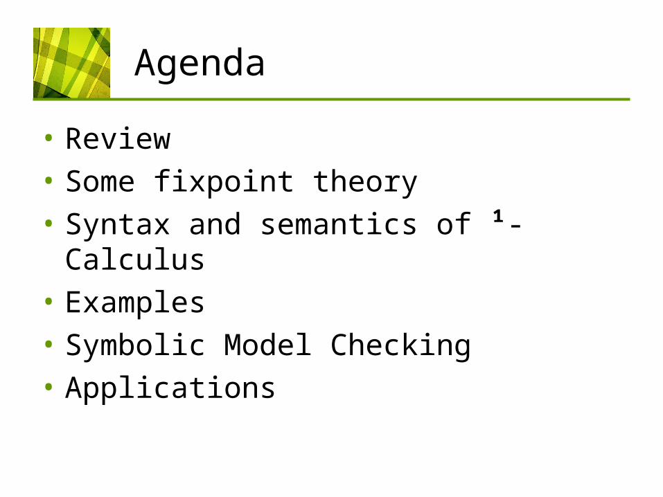
• For Y 2 VAR, Y is a formula.
• But what does it mean?
• e : VAR ! 2S is an environment
• Define: e[Q Ã W] is e with W substituted for Q– (e[Q Ã W])(Q) = W
• The environment is not needed for closed formulas

¹-Calculus Semantics (II)
• A formula f is interpreted as a set of states in which f is true
• Notation: «f¬Me
• «p¬Me = { s 2 S | p 2 L(s) }• «Y¬Me = e(Y)• «:f¬Me = S n «f¬Me• «f Æ g¬Me = «f¬Me Å «g¬Me• «f Ç g¬Me = «f¬Me [ «g¬Me
M,s ⊨ f s «f¬M

• «}f ¬Me = { s | 9t : R(s, t) Æ t 2 «f¬Me }
• «¤f ¬Me = { s | 8t : R(s, t) ! t 2 «f¬Me }
• «¹Y.f¬Me is the least fixpoint of:
¿(W) = «f¬Me[Y Ã W ]
• «ºY.f¬Me is the greatest fixpoint
¹-Calculus Semantics (II)
s s
«f¬«f¬

Restrictions on ¹-Calculus
• Are all formulae monotonic?– f Æ g, f Ç g– :f) fixpoint variables must be under an even
number of negations
¹Y . :YºY . :( Y Ç p )¹Y . :( :Y Ç p )
¿( ; ) { 1 }
¿( { 1 } ) ;
¹Y . :( :Y Ç p )¹Y . (::Y Æ :p )¹Y . (Y Æ :p )
:
¹-Calculus is closedunder negation

Agenda
• Review
• Some fixpoint theory
• Syntax and semantics of ¹-Calculus
Examples
• Symbolic Model Checking
• Applications

Why are fixpoints interesting?
• Recall from Logic I:– I( A, P ) : the smallest set W such that
•A µ W, and• If x 2 W and f 2 P then x 2 W.
– I( A, P ) = ¹Y. A Ç P( Y )
A
P

• x 2 «¹Y . ¿(Y)¬
• “Finite iteration”
• Example:– EF ' = ¹Y . ' Ç }Y
Intuition for least fixpoints
; …x

Intuition for greatest fixpoints
• x 2 «ºY . ¿(Y)¬
• “Invariant”
• Example:– EG ' = ºY . ' Æ }Y
…x x x x x=S =

• ¹Y . q Ç ( p Æ ¤Y ) = ?
A[ p U q ]
• ºY . q Ç ( p Æ ¤Y ) = ?
A[ p W q ]
¹-Calculus aerobic (I)
q
Y0Y1
p
Y2
p …

¹-Calculus aerobic (II)
• ¹Y . ºZ . ( p Æ ¤Y ) Ç ( :p Æ ¤Z ) = ?– Can pass through Y a finite number of times
• Each time p holds
– Can pass through Z infinitely• Each time p doesn’t hold
) “p is true only finitely often on all paths”

¹-Calculus aerobic (III)
• ¹Y . ºZ . ( p Æ ¤Y ) Ç ( :p Æ ¤Z ) = ?
• Inner computation 1: Y0 = ;, Z00 = S
– Z!0 = ºZ . :p Æ ¤Z = AG :p
S
p
pp
:p
:p :p :p :p …
AG :p
Notation:Yi : ith estimate for YZij : ith estimate for Z,using the jth estimate for Y! denotes the last iteration

¹-Calculus aerobic (IV)
• ¹Y . ºZ . ( p Æ ¤Y ) Ç ( :p Æ ¤Z ) = ?• Outer iteration 1:
– Y1 = ( p Æ ¤Y 0 ) Ç ( :p Æ ¤Z! 0 )
AG :p
:p :p :p :p …
AG :p

¹-Calculus aerobic (V)
• ¹Y . ºZ . ( p Æ ¤Y ) Ç ( :p Æ ¤Z ) = ?• Inner computation 2:
– Z!1 = ºZ . ( p Æ ¤Y1 ) Ç ( :p Æ ¤Z)
AG :p
:p :p :p :p …
AG :p
p: p
:p p :p …AG :p
:p
p :p :p :p …
AG :p
A[:p W ( p Æ ¤Y1 )]

¹-Calculus aerobic (VI)
• ¹Y . ºZ . ( p Æ ¤Y ) Ç ( :p Æ ¤Z ) = ?• Outer iteration 2:
– Y2 = ( p Æ ¤Y1 ) Ç ( :p Æ ¤Z! 2 )
AG :p
p :p
AG :p
Y1 Z! 2
p:p :p :p :p …
AG :p
:p p :p …AG :p
:p
p :p :p :p …
AG :p

¹-Calculus aerobic (VI)
• ¹Y . ºZ . ( p Æ ¤Y ) Ç ( :p Æ ¤Z ) = ?• Every inner computation:
A[:p W ( p Æ ¤Yn )]– Add a “layer” of :p (with infinite behaviors)
• Every outer iteration: ( p Æ ¤Yn ) Ç ( :p Æ ¤Zm )
– Add a single p

¹-Calculus aerobic (VII)
• ¹Y . ºZ . ( p Æ ¤Y ) Ç ( :p Æ ¤Z ) = ?
• p can appear a finite number of times
:p p p :p …
AG :p
:pp:p:pp p
finite no.

Agenda
• Review
• Some fixpoint theory
• Syntax and semantics of ¹-Calculus
• Examples
Symbolic Model Checking
• Applications
Symbolic Model Checking
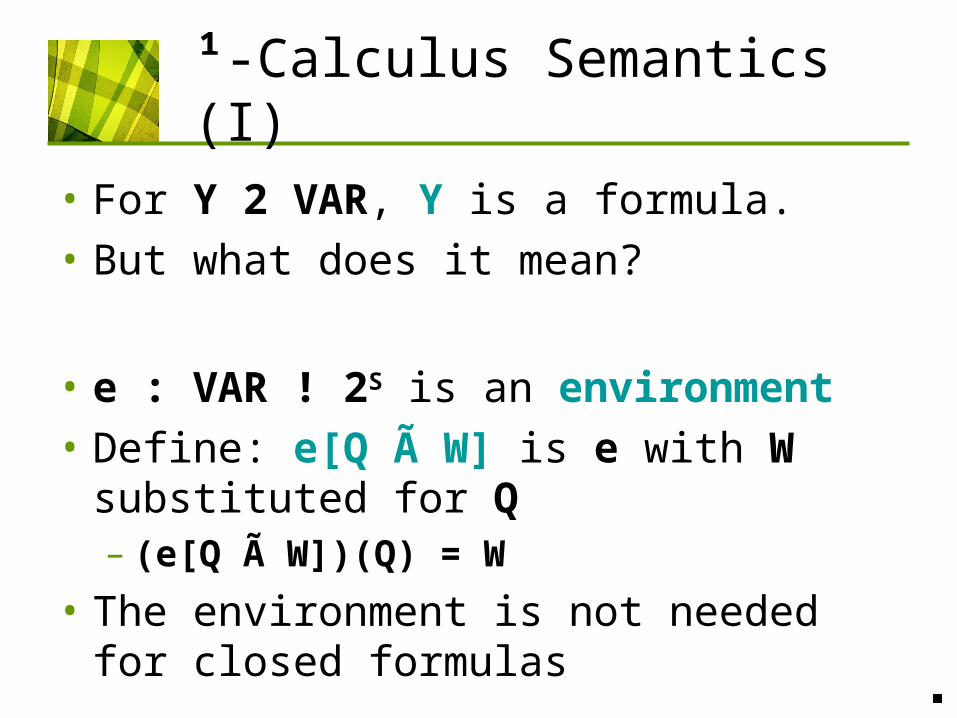
eval( f, e )
f
M, e
states thatsatisfy f

Model Checking Algorithm (I)
• if f = p :
return { s | p 2 L(s) }• if f = Q :
return e(Q)
• if f = g1 Æ g2 :
return eval( g1 , e ) Å eval( g2 , e )
• if f = g1 Ç g2 :
return eval( g1 , e ) [ eval( g2 , e )

Model Checking Algorithm (II)
• if f = } g :
return { s | 9t[R(s, t) Æ t 2 eval( g, e)] }
• if f = ¤g : return { s | 8t[R(s, t) ! eval( g,
e)(t)] }

Model Checking Algorithm (III)
• if f = ¹Y . g(Y) :
Qnew = ;
repeat
Qold = Qnew
Qnew = eval( g, e[Y Ã Qnew] )
until Qnew = Qold
return Qnew

Model Checking Algorithm (III)
• if f = ºY . g(Y) :
Qnew = S
repeat
Qold = Qnew
Qnew = eval( g, e[Y Ã Qnew] )
until Qnew = Qold
return Qnew

Model Checking Complexity (I)
if f = p :return { s | p 2 L(s) }
if f = Q :return e(Q)
if f = g1 Æ g2 :
return eval( g1 , e ) Å eval( g2 , e )
if f = g1 Ç g2 :
return eval( g1 , e ) [ eval( g2 , e )
if f = } g :return { s | 9t[R(s, t) Æ t 2 eval( g,
e)] }if f = ¤g :
return { s | 8t[R(s, t) ! eval( g, e)(t)] }
O( |M| )

Model Checking Complexity (II)
• if f = ¹Y . g(Y) :Qnew = ;repeat
Qold = Qnew
Qnew = eval( g, e[Y Ã Qnew] )
until Qnew = Qold
return Qnew
O( |S| )
O( |M| ¢ |f| ¢ |S|k)
nesting depth
Overall complexity:
Repeat entirecomputationof eval(g)

Improved Model Checking (I)
• Example: ¹Y . g(Y, ¹Z . h(Y, Z))
¹Y ¹Z
; ;
= Z ! 0 = ¹Z . h(;, Z)Y1 = g(;, Z ! 0) =
= Z ! 1 = ¹Z . h(Y1, Z)Y2 = g(Y1, Z!1) =
|S| iterations
|S| iterations
|S| iterations
O(|S|2) ) O(|S| + |S|)
Before:Now:

Improved Model Checking (II)
• What about ºY . g(Y, ¹Z . h(Y, Z)) ?
ºY ¹Z
;
= Z! 0 = ¹Z . h(;, Z)Y1 = g(;, Z ! 0) =
= Z ! 1= ¹Z . h(Y1, Z)
S

Improved Model Checking (II)
• Conclusion– Restart only on alternation
O( |M| ¢ |f| ¢ |S|k)
nesting depth
O( |M| ¢ |f| ¢ |S|d)
alternation depth
)
¹ … º … ¹ …
d

Complexity Considerations
• ¹-Calculus Model checking 2 NP Å co-NP• L = { ( M, s, f ) | M,s ² f }• A nondeterministic polynomial algorithm:
Given M, s, f,– For each greatest fixpoint in f (insideout):
• Guess a value Q• Check that Q is a fixpoint
– Model-check the rest of f• All fixpoints are ¹• Complexity: O( |M| ¢ |f | )
ºY . ¿(Y) ) Q
¿(Q) = Q

Complexity Considerations
• ¹-Calculus Model checking 2 NP Å co-NP
• Correctness:– If ( M, s, f ) 2 L, correct guess ) “yes”.– If ( M, s, f ) L:
• Suppose G is the real greatest fixpoint•Q µ G• f is monotonous• Since s «f¬,
the answer will be “no”
« f ¬
states therun will
compute

Agenda
• Review• Some fixpoint theory• Syntax and semantics of ¹-Calculus• Examples• Symbolic Model Checking
Applications– The power of ¹-Calculus– Translating CTL to ¹-Calculus– Adding fairness constraints– Checking bisimulation

¹-Calculus
The power of ¹-Calculus
CTL*
LTL CTL

CTL* vs. ¹-Calculus (II)
• Can’t express in CTL*:
“p is reachable in an even number of steps”
• In ¹-Calculus:
¹Y . p Ç }}Y
…
p
0 1 2 3 4

CTL* vs. ¹-Calculus (I)
• Can’t express in CTL*:
“p holds in every odd-numbered state on every path”
• In ¹-Calculus:
ºY . p Æ ¤¤Y
…
p p

CTL to ¹-Calculus
• AX f = ¤f • EX f = }f• EF f = ¹Y . f Ç }Y• AF f = ¹Y . f Ç ¤Y• EG f = ºY . f Æ }Y• AG f = ºY . f Æ ¤Y• E[ f U g ] = ¹Y . g Ç ( f Æ }Y )• A[ f U g ] = ¹Y . g Ç ( f Æ ¤Y )

Agenda
• Review• Some fixpoint theory• Syntax and semantics of ¹-Calculus• Examples• Symbolic Model Checking
• Applications– The power of ¹-Calculus– Translating CTL to ¹-Calculus
Adding fairness constraints– Checking bisimulation

Fairness constraints (I)
• Motivation:
p1
p2
p3
request
grantrelease
mutex
scheduler

Fairness Constraints (II)
• No starvation: “every process that requests the lock will eventually get it”
• A possible execution:
• Admissible execution: every process takes an infinite number of steps
p1
req1
p1
grant1
p2
req2
p2 p2 p2 …

Fairness Constraints (III)
• Fairness constraints:
C = ( C1, …, Ck )
• For a path ¼ = s0 s1 … :
inf(¼) = { t | t = si for an infinite number of i’s }
• A path ¼ is fair iff inf(¼) Å Ci ; for all i

Fairness Constraints (IV)
• Fairness cannot be expressed in unfair CTL
• Fair semantics:
• s ²F E ' (notation: s ² EF ') iff there exists a fair path ¼ from s such that ¼ ²F '
• s ²F A ' (notation: s ² A F ') iff for all fair paths ¼ from s, ¼ ²F '

FCTL to ¹-Calculus (I)
• EF G f = ?
ºZ . [ f Æ (Æ EX E[ f U (Ci Æ Z)] ) ]
EF G fff f
ff
C1 C2C3
n
i = 1

• EF G f = ?
ºZ . [ f Æ (Æ EX E[ f U (Ci Æ Z)] ) ]
FCTL to ¹-Calculus (II)
EF G fff f
ff
C1 C2C3
n
i = 1
fC1 C2
C3

Agenda
• Review• Some fixpoint theory• Syntax and semantics of ¹-Calculus• Examples• Symbolic Model Checking
• Applications– The power of ¹-Calculus– Translating CTL to ¹-Calculus– Adding fairness constraints
Checking bisimulation

Checking Bisimulation (I)
• Let M = ( S, s0, R, L ) and
M’ = ( S’, s0’, R’, L’ ) be Kripkestructures over AP
• H µ S’ £ S’ is a bisimulation iff forall ( s, s’ ) 2 H,
1. L1(s) = L2(s’)2. If ( s, t ) 2 R, then there exists t’ 2 S’
such that ( t, t’ ) 2 H and ( s’, t’ ) 2 R’3. If ( s’, t’ ) 2 R’, then there exists t 2 S
such that ( t, t’ ) 2 H and ( s, t ) 2 R
s s’
t t’t’t

M’M
Checking Bisimulation (II)
• M ´bis M’ if there exists a bisimulation H over M, M’ such that– For every s0 2 S0 there exists s0’ 2 S0’ such
that (s0, s’0) 2 H
– For every s0’ 2 S0’ there exists s0 2 S0 such that (s0, s’0) 2 H

Checking Bisimulation (III)
• How can we check if M ´bis M’ ?– Where will we obtain H ?
• Lemma: if M ´bis M’ then there exists a maximal bisimulation Hmax over M, M’
– If H1 and H2 are bisimulations, so is H1 [ H2
– Take Hmax = union of all the bisimulations
• Our strategy:– Compute Hmax
– Check if ( s0, s0’ ) 2 Hmax

Checking Bisimulation (IV)
• Hmax = ºH . ¿( H )
• ¿ ( H ) = H( s, s’ ) Æ8t[R( s, t ) ! 9t’( R’( s’, t’ ) Æ H( t’, t’ ) )]Æ8t’[R’( s’, t’ ) ! 9t( R( s, t ) Æ H( t, t’ ) )]
• Not a ¹-Calculus formula…
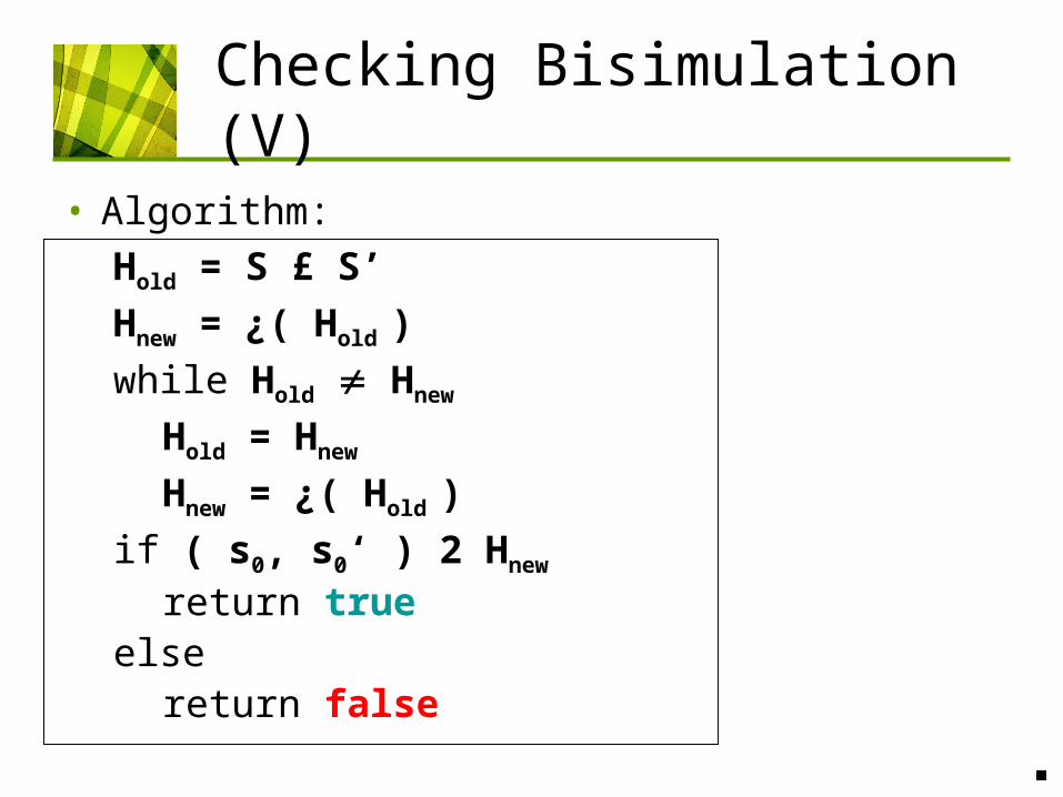
Checking Bisimulation (V)
• Algorithm:
Hold = S £ S’
Hnew = ¿( Hold )
while Hold Hnew
Hold = Hnew
Hnew = ¿( Hold )
if ( s0, s0‘ ) 2 Hnew
return trueelse
return false

Agenda
• Review
• Some fixpoint theory
• Syntax and semantics of ¹-Calculus
• Examples
• Symbolic Model Checking
• Applications
![A Multi-Encoding Approach for LTL Symbolic …...A Multi-Encoding Approach for LTL Symbolic Satisfiability Checking 3 by Clarke, Grumberg,and Hamaguchi [10], has become the de facto](https://img.pdfslide.us/doc/110x75/5f0f5afa7e708231d443bfa8/a-multi-encoding-approach-for-ltl-symbolic-a-multi-encoding-approach-for-ltl.jpg)


![[Noel Burch] Fritz Lang](https://img.pdfslide.us/doc/110x75/55cf8636550346484b954fc8/noel-burch-fritz-lang-55f058298566e.jpg)