© Boardworks Ltd 2005 1 of 53 © Boardworks Ltd 2005 1 of 53 AS-Level Maths: Core 1 for Edexcel C1.4 Algebra and functions 4 This icon indicates the slide

© Boardworks Ltd 20051 of 53 © Boardworks Ltd 20051 of 53

AS-Level Maths: Core 1for Edexcel

C1.4 Algebra and functions 4

This icon indicates the slide contains activities created in Flash. These activities are not editable.

For more detailed instructions, see the Getting Started presentation.

© Boardworks Ltd 20052 of 53

Co

nte

nts


Plotting and sketching graphs

Graphs of functions

Using graphs to solve equations

Transforming graphs of functions

Examination-style questions



Plotting graphs

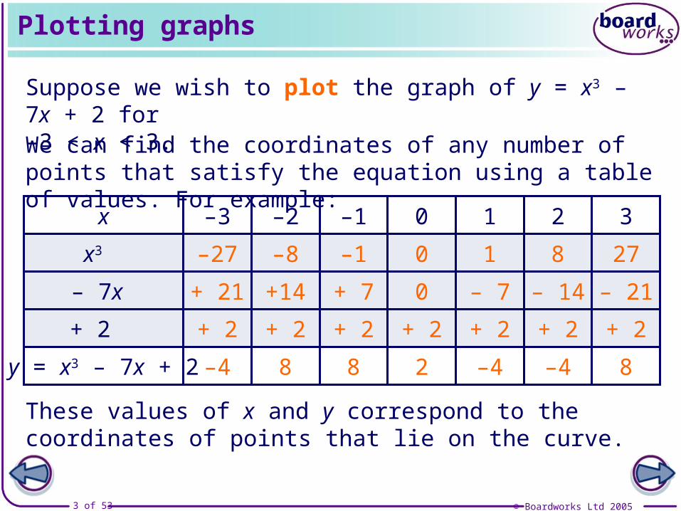
Suppose we wish to plot the graph of y = x3 – 7x + 2 for –3 < x < 3.We can find the coordinates of any number of points that satisfy the equation using a table of values. For example:

These values of x and y correspond to the coordinates of points that lie on the curve.

x

x3

– 7x

+ 2

y = x3 – 7x + 2

–3 –2 –1 0 1 2 3

–27 –8 –1 0 1 8 27

+ 21 +14 + 7 0 – 7 – 14 – 21

+ 2 + 2 + 2 + 2 + 2 + 2 + 2

–4 8 8 2 –4 –4 8


Plotting graphs

The points given in the table are plotted …

x0–2 –1–3 1 2 3

–2

–4

2

4

6

8

10

y

… and the points are then joined together with a smooth curve.

The shape of this graph is characteristic of a cubic function.

x –3 –2 –1 0 1 2 3

y = x3 – 7x + 2 –4 8 8 2 –4 –4 8


Sketching graphs

To help us sketch a graph given its equation we can find:

Points where the curve intercepts the x-axisThese are found by putting y = 0 in the equation of the graph.

Points where the curve intercepts the y-axisThese are found by putting x = 0 in the equation of the graph.

Turning pointsA turning point is a point where the gradient of a graph changes from being positive to negative or vice versa.It can be a maximum or a minimum.

The value of y when x is very large and positive

The value of y when x is very large and negative

When the general shape of a graph is known it is more usual to sketch the graph.


Sketching graphs

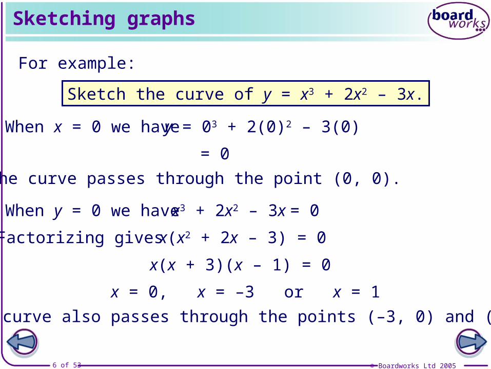
For example:

Sketch the curve of y = x3 + 2x2 – 3x.

When x = 0 we have y = 03 + 2(0)2 – 3(0)

= 0

So the curve passes through the point (0, 0).

When y = 0 we have x3 + 2x2 – 3x = 0

Factorizing gives x(x2 + 2x – 3) = 0

x(x + 3)(x – 1) = 0

x = 0, x = –3 or x = 1

So the curve also passes through the points (–3, 0) and (1, 0).


Sketching graphs

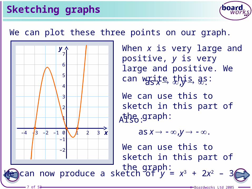
We can plot these three points on our graph.

x0–2 –1–3 1 2 3–1

–2

1

2

3

4

5

y

–4

6

7When x is very large and positive, y is very large and positive. We can write this as:

as , .x y

We can use this to sketch in this part of the graph:

Also:

as , .x y

We can now produce a sketch of y = x3 + 2x2 – 3x.

We can use this to sketch in this part of the graph:


Co

nte

nts



Graphs of functions




Graphs of functions


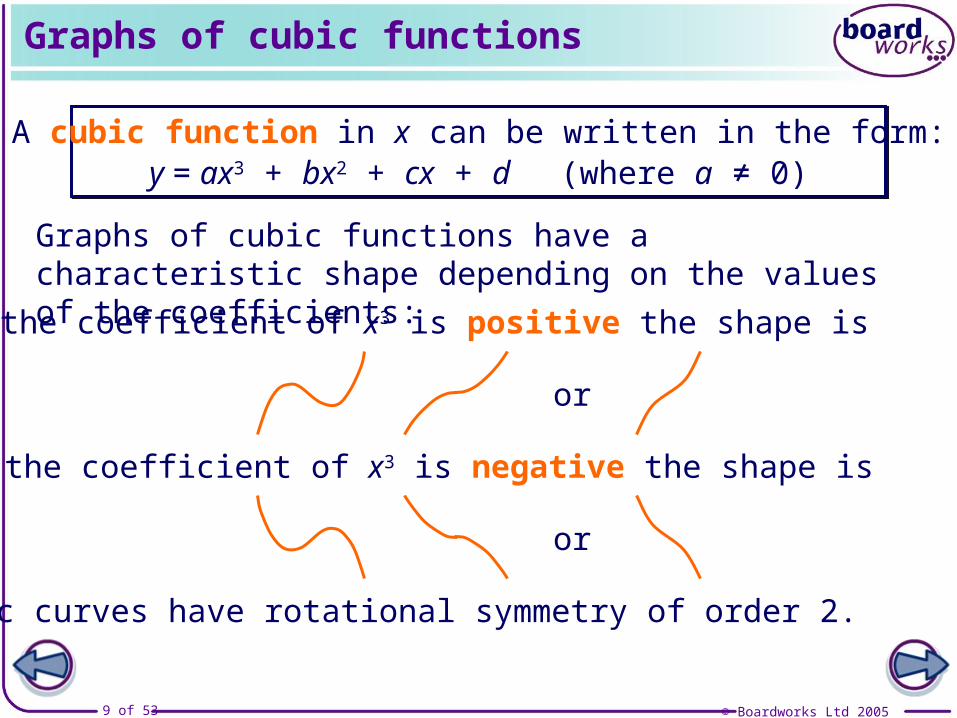
Graphs of cubic functions

y = ax3 + bx2 + cx + d (where a ≠ 0)A cubic function in x can be written in the form:

Graphs of cubic functions have a characteristic shape depending on the values of the coefficients:

When the coefficient of x3 is positive the shape is

When the coefficient of x3 is negative the shape is

or

or

Cubic curves have rotational symmetry of order 2.


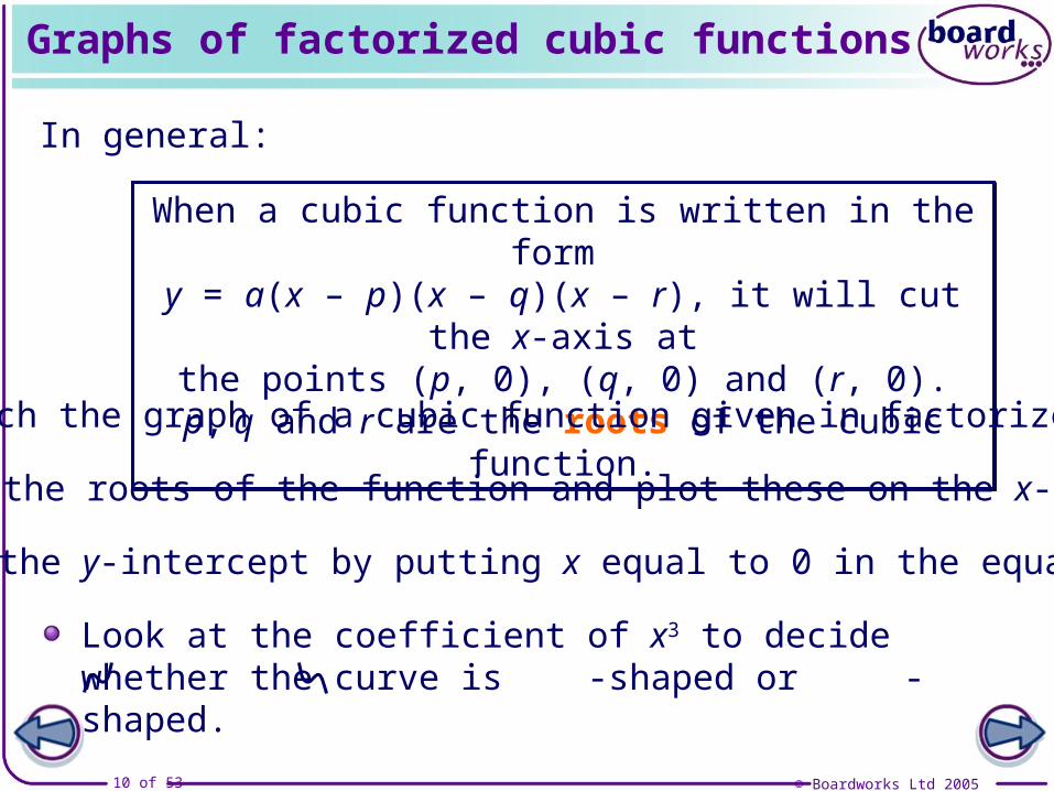
Graphs of factorized cubic functions

When a cubic function is written in the form y = a(x – p)(x – q)(x – r), it will cut the x-axis at

the points (p, 0), (q, 0) and (r, 0).p, q and r are the roots of the cubic function.

When a cubic function is written in the form y = a(x – p)(x – q)(x – r), it will cut the x-axis at

the points (p, 0), (q, 0) and (r, 0).p, q and r are the roots of the cubic function.

In general:

To sketch the graph of a cubic function given in factorized form,

Find the roots of the function and plot these on the x-axis.

Find the y-intercept by putting x equal to 0 in the equation.

Look at the coefficient of x3 to decide whether the curve is N -shaped or -shaped.


The graphs of y = x2 and y = x3

You should be familiar with the graphs of y = x2 and y = x3:

0 x

y

0 x

yy = x3y = x3y = x2y = x2

This is a quadratic function

This is a quadratic function

This is a cubic function

This is a cubic function


Graphs of the form y = kxn


0 x

y1=y

x

The graph of y = 1/x

This is a reciprocal function

This is a reciprocal function

Notice that the curve gets closer and closer to the x- and y-axes but never touches them.

The x- and y-axes form asymptotes.

1= xyYou should also be familiar with the graph of .

The graph of is an example of a discontinuous function.

1= xy


Graphs of the form y = kx–n


The graph of y =

This graph can only be drawn for positive values of x.

This is because we cannot find the square root of a negative number.

=y xAnother interesting graph is .

The curve is therefore only drawn in the first quadrant.

0 x

y

=y x

Compare this to the graph of y2 = x.

y2 = x

Also, remember that is defined as the positive square root of x.

=y x

x


Graphs of the form y = k n x


Co

nte

nts



Graphs of functions







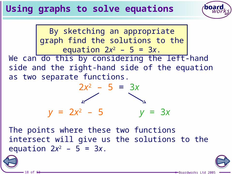
By sketching an appropriate graph find the solutions to the equation 2x2 – 5 = 3x.

We can do this by considering the left-hand side and the right-hand side of the equation as two separate functions.

2x2 – 5 = 3x

y = 2x2 – 5 y = 3x

The points where these two functions intersect will give us the solutions to the equation 2x2 – 5 = 3x.



–1–2–3–4 0 1 2 3 4–2

–4

–6

2

4

6

8

10 y = 2x2 – 5y = 3x

(–1,–3)

(2.5, 7.5)

The graphs of y = 2x2 – 5 and y = 3x intersect at the points:

The x-values of these coordinates give us the solutions to the equation 2x2 – 5 = 3x as

(–1, –3)

and (2.5, 7.5).

x = –1

and x = 2.5



Alternatively, we can rearrange the equation so that all the terms are on the left-hand side:

The line y = 0 is the x-axis. This means that the solutions to the equation 2x2 – 3x – 5 = 0 can be found where the function y = 2x2 – 3x – 5 crosses the x-axis.

2x2 – 3x – 5 = 0

y = 2x2 – 3x – 5 y = 0

These points represent the roots of the function y = 2x2 – 3x – 5.



–1–2–3–4 0 1 2 3 4–2

–4

–6

2

4

6

8

10 y = 2x2 – 3x – 5

y = 0(–1,0) (2.5, 0)

The graph of y = 2x2 – 3x – 5 crosses the x-axis at the points:

(–1, 0)

and (2.5, 0).

The x-values of these coordinates give us the same solutions:

x = –1

and x = 2.5



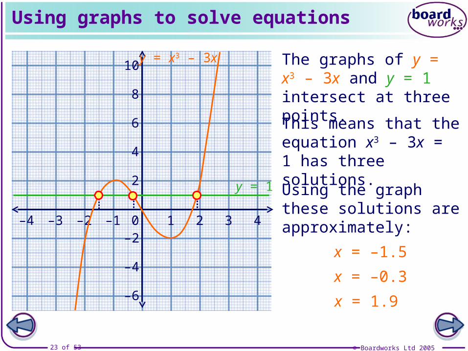
Use a graph to solve the equation x3 – 3x = 1.

This equation does not have any rational solutions and so the graph can only be used to find approximate solutions.

A cubic equation can have up to three solutions and so the graph can also tell us how many solutions there are.

Again, we can consider the left-hand side and the right-hand side of the equation as two separate functions and find thex-coordinates of their points of intersection.

x3 – 3x = 1

y = x3 – 3x y = 1


–1–2–3–4 0 1 2 3 4–2

–4

–6

2

4

6

8

10


y = x3 – 3x

y = 1

The graphs of y = x3 – 3x and y = 1 intersect at three points.

This means that the equation x3 – 3x = 1 has three solutions.

Using the graph these solutions are approximately:

x = –1.5

x = –0.3

x = 1.9


Co

nte

nts



Graphs of functions







Graphs can be transformed by translating, reflecting, stretching or rotating them.

The equation of the transformed graph will be related to the equation of the original graph.

When investigating transformations it is most useful to express functions using function notation.

For example, suppose we wish to investigate transformations of the function f(x) = x2.

The equation of the graph of y = x2, can be written as y = f(x).


x

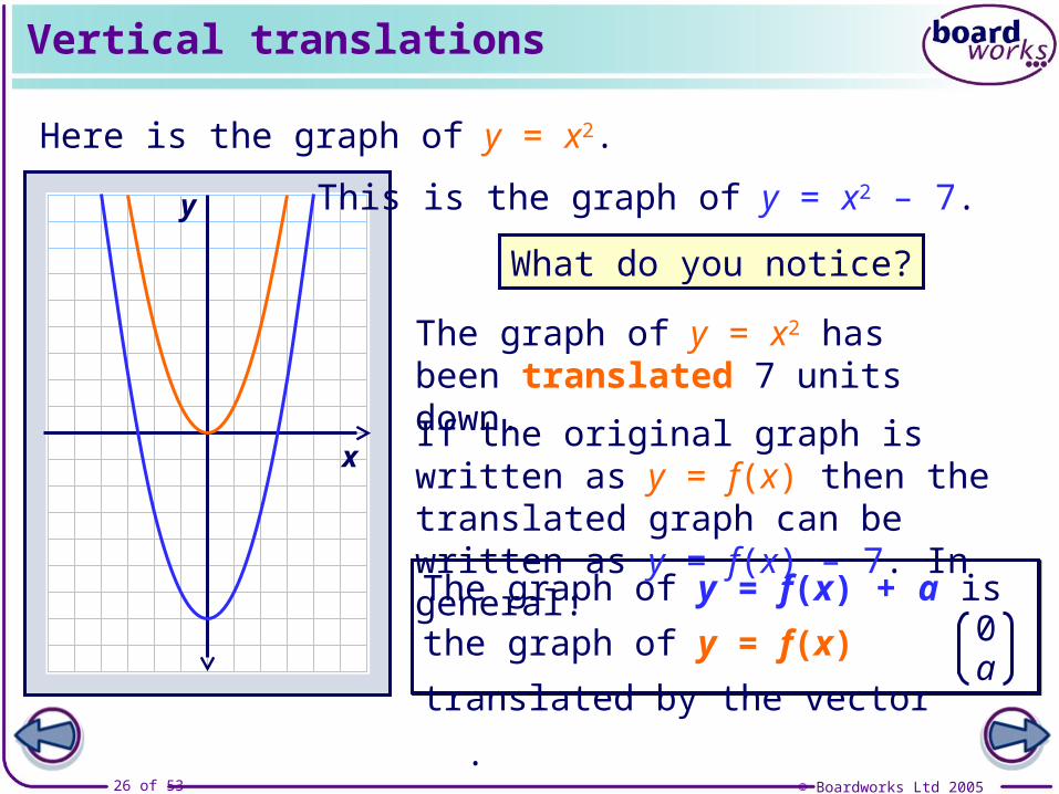
Vertical translations

This is the graph of y = x2 – 7.

What do you notice?

Here is the graph of y = x2.

y

The graph of y = f(x) + a is the graph

of y = f(x) translated by the vector .0a

The graph of y = x2 has been translated 7 units down.

If the original graph is written as y = f(x) then the translated graph can be written as y = f(x) – 7. In general:


Translating quadratic functions vertically


Translating cubic functions vertically


Translating reciprocal functions vertically


x

Horizontal translations

The graph of y = f(x + a) is the graph

of y = f(x) translated by the vector .–a0

y

Again, here is the graph of y = x2.

This is the graph of y = (x + 3)2.

What do you notice?

The graph of y = x2 has been translated 3 units to the left.

If the original graph is written as y = f(x) then the translated graph can be written as y = f(x + 3). In general:


Translating quadratic functions horizontally


Translating cubic functions horizontally


Translating reciprocal functions horizontally


x

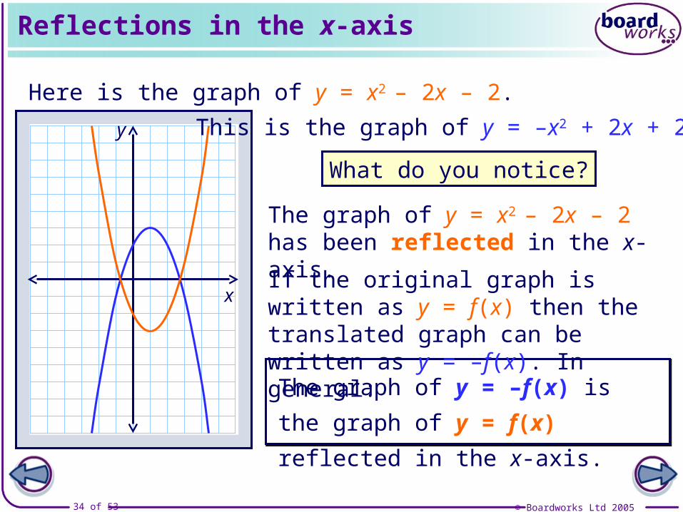
Reflections in the x-axis

The graph of y = –f(x) is the graph of

y = f(x) reflected in the x-axis.

Here is the graph of y = x2 – 2x – 2.

y This is the graph of y = –x2 + 2x + 2.

What do you notice?

The graph of y = x2 – 2x – 2 has been reflected in the x-axis.

If the original graph is written as y = f(x) then the translated graph can be written as y = –f(x). In general:


Reflecting quadratic functions in the x-axis


Reflecting cubic functions in the x-axis


Reflecting reciprocal functions in the x-axis


Reflections in the y-axis

Here is the graph of y = x3 + 4x2 – 3.

The graph of y = f(–x) is the graph of

y = f(x) reflected in the y-axis.

x

y This is the graph of y = (–x)3 + 4(–x)2 – 3.

What do you notice?

The graph of y = x3 + 4x2 – 3 has been reflected in the y-axis.

If the original graph is written as y = f(x) then the translated graph can be written as y = f(–x). In general:


Reflecting quadratic functions in the y-axis


Reflecting cubic functions in the y-axis


Reflecting reciprocal functions in the y-axis


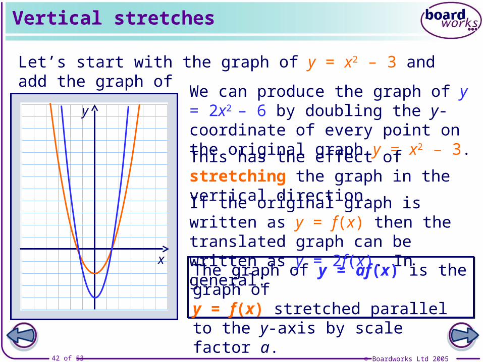
Vertical stretches

We can produce the graph of y = 2x2 – 6 by doubling the y-coordinate of every point on the original graph y = x2 – 3.

This has the effect of stretching the graph in the vertical direction.

Let’s start with the graph of y = x2 – 3 and add the graph ofy = 2x2 – 6.

The graph of y = af(x) is the graph of y = f(x) stretched parallel to the y-axis by scale factor a.

x

y

If the original graph is written as y = f(x) then the translated graph can be written as y = 2f(x). In general:


Stretching quadratic functions vertically


Stretching cubic functions vertically


Stretching reciprocal functions vertically


Horizontal stretches

The graph of y = f(ax) is the graph of y = f(x) stretched parallel to the x-axis by scale factor .a

1

x

y

Let’s start with the graph of y = x2 + 3x – 4 and add the graph ofy = (2x)2 + 3(2x) – 4.

We can produce the second graph by halving the x-coordinate of every point on the original graph.

This has the effect of compressing the graph in the horizontal direction.

If the original graph is written as y = f(x) then the translated graph can be written as y = f(2x). In general:


Stretching quadratic functions horizontally


Stretching cubic functions horizontally


Stretching reciprocal functions horizontally


Co

nte

nts



Graphs of functions






Examination-style question

This diagram shows the graph of y = f(x) which has a minimum point at (2, –3).

y

(2, –3)

a) Sketch the following graphs on separate sets of axes, indicating the turning point in each case.

i) y = f(x + 4)

ii) y = f(2x)

b) Given that f(x) = ax2 + bx + 5 find the values of a and b.

x



a) i) y = f(x + 4) ii) y = f(2x)

y

(–2, –3)

x

y

(1, –3)

x



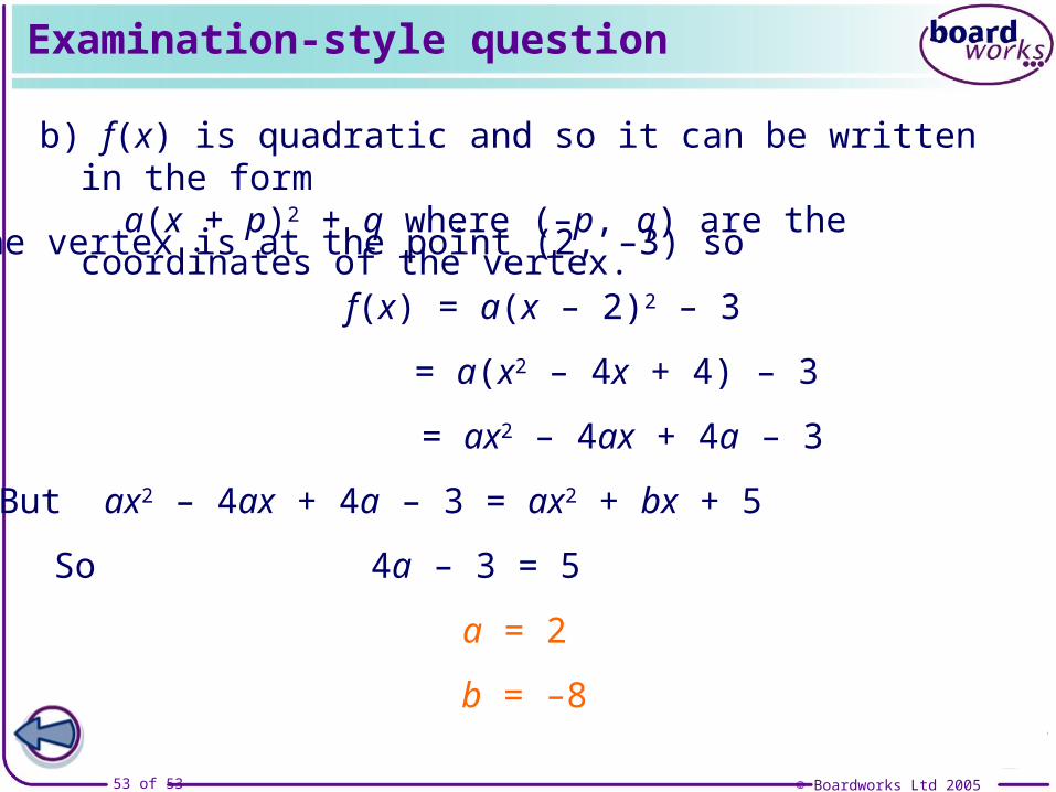
b) f(x) is quadratic and so it can be written in the form a(x + p)2 + q where (–p, q) are the coordinates of the vertex.

The vertex is at the point (2, –3) so

f(x) = a(x – 2)2 – 3

= a(x2 – 4x + 4) – 3

= ax2 – 4ax + 4a – 3

But ax2 – 4ax + 4a – 3 = ax2 + bx + 5

So 4a – 3 = 5

a = 2

b = –8

Documents

© Boardworks Ltd 2005 1 of 53 © Boardworks Ltd 2005 1 of 53 AS-Level Maths: Core 1 for Edexcel C1.4 Algebra and functions 4 This icon indicates the slide