Charles University in Prague

Faculty of Mathematics and Physics

MASTER THESIS

Bc. Filip Dvořák

AI Planning with Time and Resource Constraints

Department of Theoretical Computer Science and Mathematical Logic

Supervisor: Doc. RNDr. Roman Barták, Ph.D.

Field of study: Theoretical Computer Science

2009

  

Acknowledgements

I thank my supervisor, Doc. RNDr. Roman Barták, Ph.D., for his patient guidance and for his critical comments that helped me make this thesis better.

I thank my parents for their continuous support through the work on this thesis and through all my studies.

I hereby declare that I have written this diploma thesis on my own and solely with the use of cited references. I agree with lending and publishing of this work.

In Prague on August 6, 2009 Bc. Filip Dvořák

  

Contents

 

1  Introduction ............................................................................................................. 6 

2  Planning ................................................................................................................... 8 

2.1  Principal representations for planning ............................................................... 9 

2.2  Search techniques for planning ........................................................................ 11 

2.2.1  STRIPS algorithm ............................................................................................... 12 

2.2.2  Plan space planning ............................................................................................ 12 

2.2.3  Planning graph .................................................................................................... 14 

2.2.4  Domain transition graph ..................................................................................... 16 

2.2.5  Landmarks .......................................................................................................... 17 

3  Planning with time ................................................................................................ 19 

3.1  Qualitative and quantitative notion of time ..................................................... 19 

3.2  Temporal constraint network ........................................................................... 20 

3.3  Simple temporal problem ................................................................................ 21 

4  Planning with resources ........................................................................................ 24 

4.1  Resource categories ......................................................................................... 24 

4.2  Scheduling ....................................................................................................... 26 

4.3  Integrating planning and scheduling ................................................................ 27 

5  Planning systems ................................................................................................... 28 

5.1  CPT planner ..................................................................................................... 28 

5.1.1  Representation .................................................................................................... 28 

5.1.2  Search technique ................................................................................................. 28 

5.1.3  Summary ............................................................................................................. 29 

5.2  Constraint Network on Timelines .................................................................... 30 

5.2.1  Representation .................................................................................................... 30 

5.2.2  Search technique ................................................................................................. 31 

5.2.3  Summary ............................................................................................................. 31 

5.3  Timeline based Representation Framework .................................................... 32 

5.3.1  Component based approach ................................................................................ 32 

5.3.2  Architecture ........................................................................................................ 32 

5.3.3  Summary ............................................................................................................. 33 

6  Our planning system ............................................................................................. 34 

6.1  Conceptual model ............................................................................................ 36 

  

6.2  Simple Temporal Network............................................................................... 39 

6.2.1  Qualitative relations ............................................................................................ 40 

6.2.2  STP-minimality and incremental maintenance ................................................... 41 

6.3  Temporal databases.......................................................................................... 43 

6.4  Resource manager ............................................................................................ 44 

6.4.1  Single-capacity Reusable Resource .................................................................... 48 

6.4.2  Multi-capacity Replenishable Resource ............................................................. 48 

6.4.3  Reservoirs ........................................................................................................... 50 

6.5  Representation ................................................................................................. 53 

6.5.1  Translation .......................................................................................................... 53 

6.5.2  The planning problem ......................................................................................... 56 

6.6  Search algorithm .............................................................................................. 58 

6.6.1  Search procedures ............................................................................................... 59 

6.6.2  Improving solutions ............................................................................................ 67 

7  Testing .................................................................................................................... 68 

7.1  Domains ........................................................................................................... 68 

7.2  Competition participants .................................................................................. 69 

7.3  Testing environment ........................................................................................ 70 

7.4  Results .............................................................................................................. 71 

7.4.1  Discussion ........................................................................................................... 75 

7.5  Implementation notes ....................................................................................... 76 

8  Conclusions ............................................................................................................ 78 

8.1  Future work ...................................................................................................... 79 

Bibliography .................................................................................................................. 80 

Appendix: CD contents ................................................................................................ 84 

  

Název práce: Plánování s omezenými zdroji a časem Autor: Bc. Filip Dvořák Katedra (ústav): Katedra teoretické informatiky a matematické logiky Vedoucí diplomové práce: Doc. RNDr. Roman Barták, Ph.D. E-mail vedoucího: bartak@ktiml.mff.cuni.cz

Abstrakt: Automatizované plánování hraje bezesporu klíčovou roli v mnoha oblastech lidského zájmu, kde složité a proměnlivé úlohy vyžadují efektivní řešení a omezení možných chyb. Další motivací pro výzkum plánování je zachycení výpočetních aspektů umělé inteligence, kde plánování je jedním z klíčových elementů coby uvažování nutné k jednání. Zavedení času a zdrojů do plánování je důležitým krokem pro modelování problémů z reálného světa, nicméně plánování je samo o sobě v obecném případě velmi těžké a zavedení času a zdrojů plánování dělá ještě těžším. V této práci prozkoumáme z teoretického hlediska aspekty plánování, uvažování o čase a uvažování o zdrojích. Na základě tohoto průzkumu navrhneme vlastní suboptimální a doménově nezávislý plá-novací systém zaměřený na plánování, kde čas hraje hlavní roli, a zdroje jsou omezené. Navržený systém otestujeme na plánovacích problémech s časem a zdroji z mezinárodní plánovací soutěže roku 2008 a výsledky navrženého plánovacího systé-mu porovnáme s výsledky plánovacích systémů, které se účastnili této soutěže.

Klíčová slova: plánování se zdroji a časem, jednoduché časové sítě, grafy doménových přechodů, stavové proměnné

Title: AI Planning with Time and Resource Constraints Author: Bc. Filip Dvořák Department: Department of Theoretical Computer Science and Mathematical Logic Supervisor: Doc. RNDr. Roman Barták, Ph.D. Supervisor's e-mail address: bartak@ktiml.mff.cuni.cz

Abstract: Automated planning plays an important role in many fields of human interest, where complex and changing tasks involve demanding efficiency and error-avoidance requirements. Research in planning is also motivated by capturing the computational aspects of Artificial Intelligence, where planning, being a reasoning side of acting, is one of the key elements. Introduction of time and resources into planning is an impor-tant step towards modelling problems from the real world, however planning is generally hard and introduction of time and resources makes it even harder. In this the-sis we explore theoretical aspects of planning, temporal reasoning and resource reasoning. Based on these studies we develop our own suboptimal domain-independent planning system that focuses on planning, where time plays a major role and resources are constrained. We test the developed planning system on the planning problems with time and resources from the International Planning Competition 2008 and compare our results with the competition participants.

Keywords: planning with time and resources, simple temporal networks, domain transi-tion graphs, state variables

6  

1 Introduction

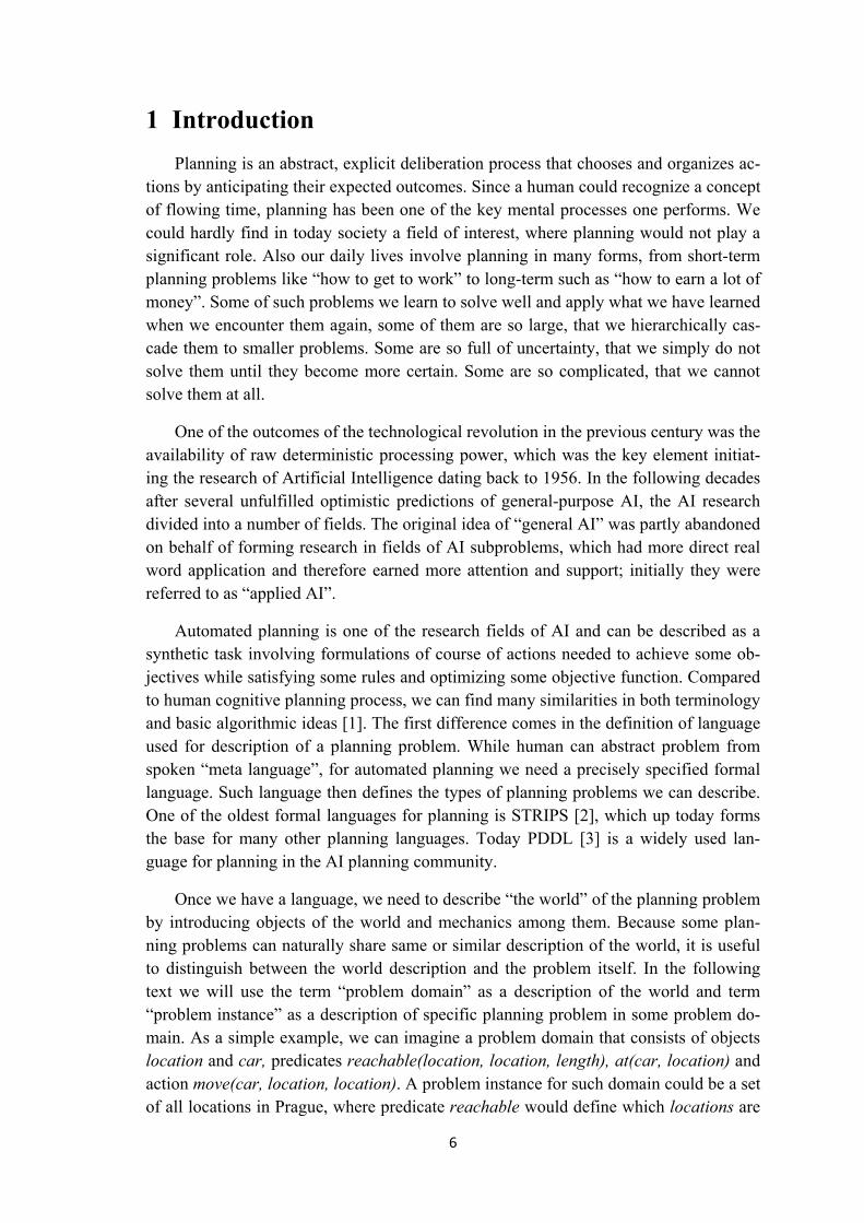
Planning is an abstract, explicit deliberation process that chooses and organizes ac-tions by anticipating their expected outcomes. Since a human could recognize a concept of flowing time, planning has been one of the key mental processes one performs. We could hardly find in today society a field of interest, where planning would not play a significant role. Also our daily lives involve planning in many forms, from short-term planning problems like “how to get to work” to long-term such as “how to earn a lot of money”. Some of such problems we learn to solve well and apply what we have learned when we encounter them again, some of them are so large, that we hierarchically cas-cade them to smaller problems. Some are so full of uncertainty, that we simply do not solve them until they become more certain. Some are so complicated, that we cannot solve them at all.

One of the outcomes of the technological revolution in the previous century was the availability of raw deterministic processing power, which was the key element initiat-ing the research of Artificial Intelligence dating back to 1956. In the following decades after several unfulfilled optimistic predictions of general-purpose AI, the AI research divided into a number of fields. The original idea of “general AI” was partly abandoned on behalf of forming research in fields of AI subproblems, which had more direct real word application and therefore earned more attention and support; initially they were referred to as “applied AI”.

Automated planning is one of the research fields of AI and can be described as a synthetic task involving formulations of course of actions needed to achieve some ob-jectives while satisfying some rules and optimizing some objective function. Compared to human cognitive planning process, we can find many similarities in both terminology and basic algorithmic ideas [1]. The first difference comes in the definition of language used for description of a planning problem. While human can abstract problem from spoken “meta language”, for automated planning we need a precisely specified formal language. Such language then defines the types of planning problems we can describe. One of the oldest formal languages for planning is STRIPS [2], which up today forms the base for many other planning languages. Today PDDL [3] is a widely used lan-guage for planning in the AI planning community.

Once we have a language, we need to describe “the world” of the planning problem by introducing objects of the world and mechanics among them. Because some plan-ning problems can naturally share same or similar description of the world, it is useful to distinguish between the world description and the problem itself. In the following text we will use the term “problem domain” as a description of the world and term “problem instance” as a description of specific planning problem in some problem do-main. As a simple example, we can imagine a problem domain that consists of objects location and car, predicates reachable(location, location, length), at(car, location) and action move(car, location, location). A problem instance for such domain could be a set of all locations in Prague, where predicate reachable would define which locations are

7  

connected by roads of certain length and predicate at would define the initial and the goal locations of the cars. If we wrote a planner for such a domain, which in this case could be a simple shortest-path graph algorithm, we would be able to switch the prob-lem instance from Prague to London, use different cars, and our planner would be able to solve such problem as well. However if we alter the problem domain, our planner will not be able to solve any problem instance. Such planner would be called domain-dependent. The planner that can solve problem instances of any domain defined in a formal language can be called domain-independent. Of course the real universality of a domain-independent planner is still constrained by the expressiveness of chosen formal language. One can predict that writing a domain-independent planner is more compli-cated than staying domain-dependent. It is, additionally independency can come with sacrifices in solution quality, additional runtime requirements and even with worse computational complexity so we can end up as Jack of all trades, master of none. Therefore, what motivation do we have for domain-independent planners? There are two main reasons. Theoretical, being able to solve planning problems for any domain from certain formal language eventually leads to creating one of the most essentials blocks of “general AI”, once the expressiveness of underlying language, hardware technology and computer science reach certain point. And practical, in many cases the performance of a domain-independent planner can be sufficient compared to the state-of-the-art domain-dependent approach and even if it is not, it is generally much easier to adapt a domain-independent planner for certain domain, therefore increasing its per-formance, than to adapt a domain-dependent planner to a significantly different domain.

Our goal in this thesis is to look into various ways of describing, representing and solving planning problems with time and resource constraints, and propose, implement and benchmark our own prototype of planning system while staying as domain-independent as possible.

In the following chapter we look into ways how a planning problem can be repre-sented, how we can search for a solution of the planning problem, and how we can further explore the structure of the planning problem. In the third chapter we describe how the structure of time can be introduced into planning and we further concentrate on quantitative notion of time and the simple temporal problem. In the fourth chapter we introduce the concept of resources, present categories of resources, and discuss how the resources are used in scheduling and planning. In the fifth chapter we describe three approaches to the integration of planning and scheduling. In the sixth chapter we intro-duce structures and algorithms used in our system. In the seventh chapter we describe the planning problems we solve and our evaluation methodology for the results, which we consequently present and discuss. We summarize our approach in the final chapter and we propose the directions for further development.

8  

2 Planning

Real world planning problems usually differ from each other significantly, various approaches were taken dealing with e.g.: path and motion planning, perception plan-ning, navigation planning, manipulation planning, communication planning or different branches of social and economic planning. These approaches often rely on their own domain representations and problem specific techniques limiting its reusability and transferability to other branches of planning problems. Finding a common ground for representing planning problems has always been a challenge as the representation of various real world features and emphasis on different aspects of problem are required.

For describing the main elements of a planning problem while leaving aside the al-gorithmic approaches it is useful to create a theoretical concept of a dynamic system. For this purpose we use a model of discrete-event system, which is also common in other areas of research, e.g. communications, industrial engineering, control theory, operational research and many branches of computer science.

Formally, a discrete-event system is a quadruple ∑ = (S, A, E, ), where:

S = {s1, s2, ...} is a finite or recursively enumerable set of states;

A = {a1, a2, ...} is a finite or recursively enumerable set of actions;

E = {e1, e2, ...} is a finite or recursively enumerable set of events; and

: S × A × E → 2S is a state transition function.

The discrete-event system can be represented as a directed graph, where nodes rep-resent states and an arc between two nodes v1 and v2 exists iff v2 (v1, a, e) for some a A and e E. It is also useful to introduce a neutral action no-action and a neutral event no-event allowing us to consider state transitions caused solely by an event or an action. While both events and actions can cause a change of the state, we use the ac-tions to describe the changes that we can control and the events to describe the uncontrollable changes. The purpose of planning is to find which actions to apply to which states to achieve some objective when starting from some given situation. Using our simple domain from introduction, we can imagine an event to be a change, which e.g. arbitrary disables some road.

For purpose of this thesis we will additionally constrain this model by several as-sumptions:

We assume we have a complete knowledge of the system. This assumption can also be referred to as a fully observable system; contrary without this assump-tion, we would be referring to planning with uncertainty.

9  

We assume that the set of events is empty. The system can be called static; ad-ditionally we are not concerned with any changes that may occur while we are planning. In other words we are planning offline.

We assume the system to be deterministic by considering the transition func-tion to always bring a deterministic system to a single other state.

While our model of the discrete-event system might seem sufficient for the descrip-tion of a planning problem, it is not feasible, except for the most trivial cases, to represent all states explicitly due to combinatorial explosion of enumeration. Consider-ing our toy-example, with 30 cars and 100 locations our graph would have 1060 nodes. Hence it is essential to work with a compact implicit representation, which would de-scribe useful subsets of state space and allow an effective searching approach.

2.1 Principal representations for planning

In planning we can generally find three principal concepts of representation: set-theoretic, classical and state-variable [4]. These representations are equal in its expres-sive power and transferable among each other. We can usually refer to them as “classical representations”. While techniques discussed in this thesis are building upon more compound representations, we will use classical representations as a reference point.

In a set-theoretic representation, each state of the world is a set of propositions, and each action is a syntactic expression specifying which propositions belong to the state in order for the action to be applicable and which propositions the action will add or remove in order to make a new state of the world. We can represent actions as a triple (preconditions, negative effects, positive effects).

In a classical representation, the states and actions are like the ones described for set-theoretical representations except that first-order literals and logical connectives are used instead of propositions.

In a state-variable representation, each state is represented by a tuple of values of n state variables {x1, x2, ..., xn}, and each action is represented by a partial function that maps this tuple into some other tuple of values of the n state vari-ables.

Using our toy-example, we can create representations for the following problem. We assume we have cars car1, car2 and locations loc1, loc2, initially car1 is at loc1 and car2 is at loc2. Our objective is to swap the locations of the cars. Figure 2.1 depicts the formulation of problem in the three representations.

10  

set-theoretic representation propositions: {car1-loc1, car1-loc2, car2-loc1, car2-loc2} actions: move-car1-loc1-loc2({car1-loc1}, {car1-loc1}, {car1-loc2}) move-car1-loc2-loc1({car1-loc2}, {car1-loc2}, {car1-loc1}) move-car2-loc1-loc2({car2-loc1}, {car2-loc1}, {car2-loc2}) move-car2-loc2-loc1({car2-loc2}, {car2-loc2}, {car2-loc1}) initial state: {car1-loc1, car2-loc2} goal state: {car1-loc2, car2-loc1} classical representation constants: {car1, car2, loc1, loc2} predicates: {car(x), loc(x), at(x, y)} operators: move(x, y, z): preconditions: car(x), loc(y), loc(z), at(x, y) effects: not at(x, y), at(x, z) initial state: {car(car1), car(car2), loc(loc1), loc(loc2), at(car1, loc1), at(car2, loc2)} goal state: {at(car1, loc2), at(car2, loc1)} state-variable representation objects: car {car1, car2}, loc {loc1, loc2} state variables: at(car, loc): states × car → loc operators: move(x car, y loc, z loc): preconditions: at(x) = y effects: at(x) = z initial state: {at(car1) = loc1, at(car2) = loc2} goal state: {at(car1) = loc2, at(car2) = loc1}

Figure 2.1: Example of different representations of the toy-problem with two cars and two locations.

Classical and state-variable representations are more expressive than the set-theoretic representation in sense of amount of information they can encode, although all three representations can still encode the same set of planning domains. While in the set-theoretic representation we are grounding all elements, in classical and state-variable representations we gain additional information by e.g. encoding position of a car as a single valued function through state-variable, which is more natural in sense that one car cannot occur at several locations at once. If we restrict all atoms and state-variables to be ground, these representations would be essentially equivalent allowing translation to each other with at most linear increase in size [4].

 

11  

2.2 Search techniques for planning

Among the first decisions that come in question when we think about searching for a plan is the specification of the search space. There are generally two concepts of search space; either we can search through the space of states of the system or we can search through the space of partially specified plans. While in the space of states the edges represent the transitions between the states caused by an action or an event, in plan space the edges represent the refinement operations intended to further complete a partial plan. In theory, planning in plan space can be seen as a generalization of state space planning. One can imagine a choice of the applicable action being a refinement of a plan.

Planning is generally hard, PSPACE-complete for a restricted case, where actions are limited to a single non-negated precondition [5]. Consequently searching for opti-mal plans is much harder than searching for feasible plans; therefore many today competitive domain-independent planning systems are incomplete incorporating some form of non-admissible heuristic. In practice we often do not need optimal plans, which are sometimes too hard to find, and we resort to plans which are good in sense of some measurable quality.

How do we measure the quality of a plan? In the beginning of automated planning research there was actually a single criterion, the existence of a plan, therefore finding any plan was sufficient and formulated planning problems reflected it. Later, with the increased spectrum of problems, planning community became interested not only in finding plans, but also in finding particularly good plans. An obvious measure for qual-ity can be the length of a plan, in other words, the number of actions used to reach a goal state from the initial state. Alternatively we can associate a cost with each action and represent plan quality as a sum of all action costs in a plan. Once we extend plan-ning with time, we can use the total time of a plan as the measure of quality. Extending planning with resources brings another way how to measure quality through objective function on evolution of resource usage. We can extend a planning problem with some form of preferences or soft constraints and measure the number of their possibly weighted violations. In this thesis we usually stick to a single criterion, although in practical application it is useful to combine several measurements methods, e.g. to minimise the total-time and soft-constraint violations, especially in cases when a human planner is a part of the planning process.

In this section we start by introducing STRIPS algorithm as a principal representa-tive of the state space planning. Consequently we describe planning in the plan space, introduce the concepts of two useful structures, a planning graph and a domain transi-tion graph, and finally we describe the concept of landmarks.

 

12  

2.2.1 STRIPS algorithm

Searching for a plan in state space we can generally think of two concepts, we can either search for a way from the initial state to the goal state or from the goal state to the initial state. Those concepts are usually referred to as “forward search” and “back-ward search”. The strategy of choosing the next state in a search is the defining point of a state space planning system.

The pioneering planner in state space planning was Stanford Research Institute Problem Solver, shortly STRIPS, developed in 1971 [2]. Its initial practical purpose was a control of a small robot, planning and performing simple tasks. Due to limited processing power at that time it was essential to significantly prune the state space; therefore the original algorithm was incomplete. STRIPS algorithm can be conceptually described as follows:

1. Extract the differences between the current state and the goal state.

2. Identify relevant operators for reducing these differences.

3. Solve the subproblem of producing a state where such a relevant operator can be applied.

4. Repeat until all goals are satisfied.

The heuristic choice of relevant operator in step 2 is based on difference measure-ment, which consists of the number of remaining goals and the number and types of remaining predicates in the remaining goals. Step 3, in other words, represents solving all preconditions of operator chosen at step 2. One of well known downsides of the STRIPS algorithm is Sussman anomaly, which occurs, when an operator solving a pre-condition deletes one of already achieved goals. STRIPS algorithm and its different extensions are up today still heavily used in practice, e.g. in computer games. Later developed formal language of inputs for STRIPS planner is the base for most languages used today for expressing planning problems.

2.2.2 Plan space planning

Plan space planning differs from state space planning not only in the search space but also in the description of a solution plan, which is no longer a sequence of actions but a set of partially instantiated operators together with ordering constraints and bind-ing constraints. Formally, a partial plan is a quadruple π = (A, , B, L), where:

A = {a1, a2, ..., ak} is a set of partially instantiated planning operators.

is a set of ordering constraints on A of the form (ai aj)

B is a set of binding constraints on the variables of actions in A of the form x = y, x ≠ y, or x Dx, where Dx is a subset of the domain of x.

13  

L is a set of causal links of the form , such that ai and aj are actions in

A, the constraint (ai aj) is in , proposition p is an effect of ai and precondi-tion of aj, and the binding constraints for variables of ai and aj appearing in p are in B.

The search space is an implicit directed graph, whose nodes are partial plans and whose edges correspond to refinement operations. A refinement operation consists of one or more additions of following into a partial plan: an action into A, an ordering constraint into , a binding constraint into B or a causal link into L.

The addition of an action into a partial plan performs a refinement by supporting one of the subgoals, which can be either a plan goal or a condition of another previ-ously added action. Because initial and goal states are usually represented as a set of actions with no preconditions, respectively no effects, we consider the reason for an addition of action being always support for the precondition of another action. Added action also needs to happen before the action, whose condition it supports, therefore we need to add an ordering constraint between these two actions. Consequently we would like to ensure, that another action does not delete the supported proposition after it gained its support but before it was needed. Therefore we are adding a causal link be-tween the two actions marking it with the proposition and we determine if the added action does threaten any other already existing causal links, which would have to be later solved as a flaw of the partial plan. Finally adding the binding constraints ensures that both the supported and the supporting action are concerned with the same atomic proposition.

Search in plan space planning can be conceptually described as a loop over solving flaws in a partial plan, where a flaw can be an unsupported precondition of an action, or an action threatening some causal link. A threat to an existing causal link can be re-solved by either binding threatening action before or after both actions forming the causal link or adding binding constraints to the variables of the threatening action such that the conflict proposition of the causal link is not threatened. The search strategy in plan space planning is determined by decision points, which are the choice of the flaw to solve, the choice of supporting action for certain precondition and the choice of a way of resolving a threatened causal link.

Once all flaws of a partial plan are resolved and and B are consistent, we have found a set of plans, from which we can extract the final ground plan. However the extraction itself can be another search problem, according to some measurement of plan quality.

Comparing state space planning and plan space planning, we can find the following main differences:

Nodes in plan space search are generally more computationally demanding. While in state space we compute just the transition function, the refinement op-

14  

erations in plan space may involve expensive consistency checking and threat management.

In state space planning the solution plan is a sequence of actions, while in plan space planning the structure of the solution plan is a set of partially ordered ac-tions. Therefore plan space planning can be extended with the concept of time and concurrent actions more naturally.

In plan space the notion of explicit states during search is lost; therefore it is generally harder to benefit from domain-specific heuristic and control knowl-edge.

2.2.3 Planning graph

The solution plans in state space planning consisted of a sequence of actions; in plan space planning the solution plans represented a set of partially ordered actions. Planning graph techniques take the middle ground with a plan being represented by a sequence of sets of actions. While plan space planning maintains a least commitment approach with partially instantiated and partially ordered actions, planning graph ap-proaches make strong commitments with fully instantiated and positioned actions. The approaches rely on two powerful and interrelated ideas: reachability analysis, which addresses the issue of whatever a state is reachable from some given state, and disjunc-tive refinement, which addresses the flaws through the disjunction of resolvers.

In state space we can define reachability of state s1 from state s0 in k steps by creat-ing a reachability tree of depth k, whose nodes are the states and edges correspond to the applicable actions. Such tree then also solves any planning problem from state s0 with the number of actions less or equal to k. Since some nodes can be reached by dif-ferent paths, the reachability tree can be factorized into a graph. However even such a reachability graph grows quickly with increasing k and eventually covers all reachable states in the state space.

The major contribution of the planning graph technique is the relaxation of reach-ability. While the reachability graph gives a sufficient condition, the planning graph gives only necessary condition for reachability. However the planning graph is of poly-nomial size and can be computed in polynomial time in the size of input.

The leading idea of the planning graph structure is to consider every level of the hypothetical reachability tree not as specific states but as a union of propositions in those states. While in the reachability graph a node is associated with the propositions that necessarily hold for that node, in the planning graph a node contains propositions that possibly hold. However the union of sets of propositions for several states does not preserve consistency, e.g. using our toy-example, we could have a car at several loca-tions at once. We can solve this by keeping a track of incompatible pairs of propositions.

15  

The planning graph is a directed layered graph, where arcs exist only from one layer to the next. Nodes in level 0 represent propositions of the initial state s0 of a plan-ning problem. Every further level contains two layers, an action layer and a proposition layer. The action layer contains a set of actions whose preconditions are nodes in the previous proposition layer. The proposition layer contains a set of positive effects of actions from the previous layer. An action node in an action layer is connected with incoming arcs from its preconditions in the previous layer and with outgoing arcs to its positive and negative effects in the next layer. Since our goal is to represent multiple states in state space, we consider negative effects of actions to be non-deleting; addi-tionally we need to carry persistent propositions between the proposition layers, therefore we enrich a set of actions by no-op actions, where for each proposition a no-op action’s single precondition and positive effect is the proposition.

For defining the incompatibility of propositions and actions, we start with the defi-nition of dependency between actions. We say that two actions a and b are depend iff either of the following holds:

effects-(a) [precond(b) effects+(b)] ≠ or

effects-(b) [precond(a) effects+(a)] ≠ .

Where effects- and effects+ denote negative and positive effects of an action. Con-sequently two actions are independent if they are not dependent and a set of actions is independent if it is pair-wise independent.

The incompatibility relation between actions and between propositions in a plan-ning graph is defined as follows:

Two actions a and b in an action layer are incompatible if either a and b are de-pendent or if a precondition of a is incompatible with a precondition of b.

Two propositions p and q in the proposition layer are incompatible, if every ac-tion in the previous action layer that has p as a positive effect (including no-op actions) is incompatible with every action that produces q, and there is no ac-tion that produces both p and q.

While dependency of actions is a static property of the problem domain, incompati-bility relations take into account additional constraints of the problem. Furthermore propositions and actions in a planning graph monotonically increase from one level to the next, while incompatible pairs monotonically decrease. These monotonic properties are essential for the complexity and termination of the planning graph techniques, which is further discussed e.g. in [4].

A layered plan is a sequence of sets of actions, which is a solution of planning prob-lem iff each set of actions is independent and sequentially applicable to the initial state.

16  

Planning graph was introduced as a part of GraphPlan planner [6], which performed significantly better than previous state space planners. Additionally the richness of the planning graph structure opened a way to broad development of extensions and re-search, and consequently brought significant improvement of performance, in sense of scalability and efficiency, in state space planning.

2.2.4 Domain transition graph

The concept of domain transition graph is strongly related to the state variable rep-resentation. The domain of a single state variable is a set of values, which the state variable can attain. Informally, the domain transition graph for certain state variable is a directed graph, where nodes represent values from the state variable domain and arcs represent actions, whose effects contain assignment of value for the state variable. The concept of domain transition graphs was firstly introduced in [7] as a part of SAS+ rep-resentation; recently it was extended with conditional effects and axioms in [8] as a part of Multi-valued Planning Task representation used in Fast Downward planner.

The benefit of state variable representation is an aggregation of mutually exclusive, shortly mutex, propositions into state variables. This aggregation can be done initially in the definition of the planning domain. However sometimes it may not be an easy and natural task for a human planner to explore and formulate state variables in a range of its possible coverage. The reason is that the state variables may no longer be interpreted as a simple description of some meaningful real world feature. Therefore generating state variables automatically is desirable.

A technique for generation of state variable developed in [8] relies on the concept of invariant synthesis. Generally, invariant in a planning problem is a property of the world state, which is satisfied in all world states reachable from the initial state. Invari-ants in planning have been studied in different contexts, usually in SAT-based planning, e.g. in [9]. For the purpose of state variables generation we are especially interested in mutex invariant, which holds the information, that a certain set of proposi-tions is pairwise mutually exclusive and therefore can be encoded as a single state variable. However we have to deal with two additional problems. Invariants discovery and proving is generally hard; in fact it can be as hard as planning itself. Consequently once we discover mutex invariants defining sets of mutex propositions, these sets will share propositions, and since our goal is to generate as few state variables as possible, while covering all propositions, we have obtained a set covering problem, which is in this case NP-complete.

Multiple approaches to mutex invariant synthesis have been introduced in literature, e.g. in [9] and [10]. Although the discovery is generally hard, a slightly relaxed ap-proach of form “guess and check” is often reasonably productive. Similarly a simple greedy algorithm produces suitable coverage of the mutex sets for purpose of state vari-ables. Afterall, we cannot spend all the time creating optimal representation and leave

17  

no time to planning itself. Due to space limitation we do not describe specific ap-proaches to invariant synthesis in detail.

For illustration we can extend our toy-example with passengers who can either walk or drive between locations. While driving requires a road, walking does not; however walking takes longer, hence walking between certain locations is not an option. Assum-ing we have three locations, one car and one passenger, possible domain transition graphs are depicted in Figure 2.2.

Figure 2.2: Domain transitions graphs for a problem with three locations, one car and one passenger.

2.2.5 Landmarks

Landmarks are facts that must be true at some point in every valid solution of a planning problem. Since the validity of a solution requires all goals to be satisfied, we can see the goals as trivial landmarks. One motivation for landmarks can be decomposi-tion of a possibly large planning problem into smaller subproblems, which would exponentially speed up the planning process. However such decomposition may not always be possible or effective due to high interdependency among the landmarks. Planning system SGPlan takes this lead and its version SGPlan6 won the recent IPC in deterministic temporal satisfaction track [11].

As usual in automated planning, finding all landmarks can be hard. Additionally the contribution of landmarks itself may not be as large, unless we can find some orderings between them. The goal ordering is one of the longstanding issues in automated plan-ning. Among the recent contributions to a problem of goal ordering we find [12], where authors introduce concepts of several orderings, which were later extended for land-marks in [13]. Another extension of landmarks, proposed in [14], was used in heuristic planning system LAMA, which won the recent IPC in deterministic sequential satisfac-tion track [11].

18  

Some landmarks can be found easily, goals are essentially landmarks. In case we are working with domain transition graphs, we can efficiently extract additional land-marks from the graph; assuming there is an initial node and a goal node in the graph then a landmark is a node, which is contained in every path from the initial node to the goal node. One of general techniques for landmark extraction is backchaining. We de-scribe the backchaining with using relaxed planning graph as proposed in [13].

The planning graph is built as described earlier; the relaxation consists of ignoring all negative effects of actions. Hence there are no incompatibility relations in the graph, which now encodes an overapproximation of reachability. Using backchaining, we start with some landmark (may be a goal) and search through the preconditions of the “earli-est” actions that achieve the landmark; any precondition shared among all the earliest actions is a candidate to be a landmark, where “early” is a greedy approximation of reachability from the initial state. Consequently we can order newly found candidates before the initial landmark. The process is iterated unless there are no new candidates. Consequently the candidates we found are evaluated. The sufficient condition for a candidate to be a landmark is based on solving the relaxed task; using the relaxed plan-ning graph, we remove all actions that can add the candidate and if the task becomes unsolvable, we have found a landmark.

An extension proposed in [14] uses a more general concept of landmark. Instead of single proposition being a landmark, we can consider a set of disjunctive propositions forming a landmark; hence a disjunctive landmark. While such disjunctive landmark cannot be easily used as a subgoal, it can still be beneficially used for leading a search algorithm, e.g. by measuring the distance from a goal by the number of disjunctive landmarks that have not been achieved.

For illustration we can imagine an example problem of a passenger, who needs to get from some location A in a city, which has an airport at location E and a shipyard at location D, to location G in another city, which has both airport and shipyard at location F. Figure 2.3 depicts landmarks we may find.

Figure 2.3: Example of landmarks found in the travelling example, A and B are trivial landmarks, {C,D} and {E,D} are disjunctive landmarks, B and F are discovered through domain transition graph.

 

19  

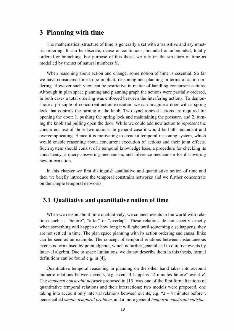
3 Planning with time

The mathematical structure of time is generally a set with a transitive and asymmet-ric ordering. It can be discrete, dense or continuous, bounded or unbounded, totally ordered or branching. For purpose of this thesis we rely on the structure of time as modelled by the set of natural numbers .

When reasoning about action and change, some notion of time is essential. So far we have considered time to be implicit, reasoning and planning in terms of action or-dering. However such view can be restrictive in matter of handling concurrent actions. Although in plan space planning and planning graph the actions were partially ordered, in both cases a total ordering was enforced between the interfering actions. To demon-strate a principle of concurrent action execution we can imagine a door with a spring lock that controls the turning of the knob. Two synchronized actions are required for opening the door: 1. pushing the spring lock and maintaining the pressure, and 2. turn-ing the knob and pulling open the door. While we could add new action to represent the concurrent use of those two actions, in general case it would be both redundant and overcomplicating. Hence it is motivating to create a temporal reasoning system, which would enable reasoning about concurrent execution of actions and their joint effects. Such system should consist of a temporal knowledge base, a procedure for checking its consistency, a query-answering mechanism, and inference mechanism for discovering new information.

In this chapter we first distinguish qualitative and quantitative notion of time and then we briefly introduce the temporal constraint networks and we further concentrate on the simple temporal networks.

3.1 Qualitative and quantitative notion of time

When we reason about time qualitatively, we connect events in the world with rela-tions such as “before”, “after” or “overlap”. These relations do not specify exactly when something will happen or how long it will take until something else happens; they are not settled in time. The plan space planning with its action ordering and causal links can be seen as an example. The concept of temporal relations between instantaneous events is formalised by point algebra, which is further generalised to durative events by interval algebra. Due to space limitations, we do not describe them in this thesis, formal definitions can be found e.g. in [4].

Quantitative temporal reasoning in planning on the other hand takes into account numeric relations between events, e.g. event A happens “2 minutes before” event B. The temporal constraint network proposed in [15] was one of the first formalizations of quantitative temporal relations and their interactions; two models were proposed, one taking into account only interval relations between events, e.g. “2 – 8 minutes before”, hence called simple temporal problem, and a more general temporal constraint satisfac-

20  

tion problem, which allowed disjunctive relations, e.g. “2 - 3 or 7 – 8 minutes before”. Both models are widely used, e.g. in medical informatics, air traffic control and auto-mated planning and scheduling. We describe both models in the next two sections.

3.2 Temporal constraint network

Temporal constraint satisfaction problem, shortly TCSP, is built upon constraint satisfaction problem formalism [16]. Formally, TCSP is a kind of CSP, where:

{x1, ..., xn} is a set of variables, whose domains are in ; each variable repre-sents a time point.

{c1, ..., cm} is a set of unary and binary constraint, where each constraint is rep-resented by a set of intervals {[a1, b1], ..., [ak, bk]}.

A unary constraint restricts the domain of a variable to the given set of intervals; it represents the disjunction (a1 ≤ xi ≤ b1) ... (ak ≤ xi ≤ bk).

A binary constraint restricts the permissible values for the distance xj – xi; it repre-sents the disjunction (a1 ≤ xj - xi ≤ b1) ... (ak ≤ xj – xi ≤ bk).

Since we usually need to relate time points to some global starting point, the “be-ginning of the world”, it is useful to add a variable representing it. Such variable x0 than allows to rewrite unary constraints on variables to binary constraints representing the distance from x0, whose domain is restricted to a single value.

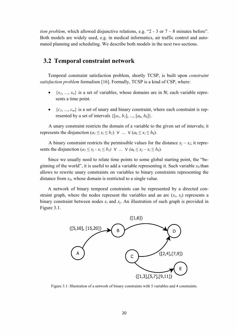
A network of binary temporal constraints can be represented by a directed con-straint graph, where the nodes represent the variables and an arc (xi, xj) represents a binary constraint between nodes xi and xj. An illustration of such graph is provided in Figure 3.1.

Figure 3.1: Illustration of a network of binary constraints with 5 variables and 4 constraints.

 

21  

Given a constraint network we are usually interested in the following questions:

Is the network consistent?

What is the minimal domain of xi?

What is the minimal constraint between xi and xj?

Generally all these questions are NP-hard. An algorithm proposed in [4] can find a minimal network in O(n3ke), where n is a number of nodes, k is the maximal number of intervals any constraint can have and e is the number of arcs. Other algorithms for con-sistency checking are proposed e.g. in [16].

In this thesis we are interested in a special case of TCSP, where each constraint is limited to single interval. This case is known as simple temporal problem, shortly STP. For simplicity we formalise operations on STP instead of TCSP, the reader may find appropriate formal definitions for TCSP e.g. in [16].

3.3 Simple temporal problem

In STP every binary constraint between two time points (xi,xj) represents a minimal and maximal distance between them; we can write such constraint as a ≤ xj - xi ≤ b. A simple temporal problem is a pair (X,C), where:

X = {x1, ..., xn} is a set of time point variables in the same sense as in TCSP.

C is a set of intervals, where each interval rij = [aij, bij] represents the constraint between time point variables xi and xj of the form aij ≤ xj - xi ≤ bij.

Consequently we can see that [aij, bij] = [-bji, -aji]. The composition and intersection operations are defined as follows:

Composition: rij · rjk = [aij + ajk, bij + bjk], which corresponds to the sum of the two constraints: aij + ajk ≤ xj - xi + xk - xj ≤ bij + bjk → aik ≤ xk - xi ≤ bik.

Intersection: rij r’ij = [max{aij, a’ij}, min{bij, b’ij}], which represents the con-junction max{aij, a’ij} ≤ xj - xi ≤ min{bij, b’ij}.

We say that STP (X,C) is consistent if there exists at least one solution that satisfies all constraints, where a solution is an assignment of values to time point variables of the form (x1 = v1, ..., xn = vn). We call the problem of deciding, if a given instance of STP is consistent, the STP-consistency.

Since constraints given in some general instance of STP may not represent the ac-tual time between two time points and deciding consistency through searching for possible assignments of values to time point variables is not very effective, we try to

22  

reduce the constraints with transitive closure operation defined as: rij ← rij (rik · rkj). An example of such reduction is shown in Figure 3.2.

Figure 3.2: Example of transitive closure propagation; since event C happens at least 1 time unit after event B and event B happens at least 5 time units after A, we deduce that event C happens at least 6 time

units after event A; similarly for maximal time distance.

The propagation of transitive closure upon consistent STP tightens constraints to its minimal form. Such constraint network is then called minimal in sense that every point in any interval rij belongs to some solution. The minimal network has a desirable prop-erty that any solution can be extracted without backtracking, simply by choosing step by step variable assignments satisfying all constraints from already assigned variables; while minimality of the network guarantees that there will always be a set of values to choose from. We refer to the problem of finding minimal network as STP-minimality. For example in Figure 3.2 we have achieved a minimal network.

STP-minimality from the definition implies STP-consistency; also minimal network for inconsistent STP is not defined. Due to deep research in CSP field we can find vari-ous algorithms with different properties for solving both STP-minimality and STP-consistency. Since propagation of transitive closure solves STP-minimality, the most notable are path-consistency algorithms. A simple case of path-consistency algorithm for purpose of STP-minimality is the Floyd-Warshall algorithm, which finds shortest paths among all nodes in a graph; in our case the tightest constraints.

Algorithm 3.1 – Floyd-Warshall algorithm for STP

01 F-W(STP = (X,C))

02 foreach xi X

03 foreach xj X \{xi}

04 foreach xk X \{xi,xj}

05 rij ← rij (rik · rkj)

The Floyd-Warshall algorithm computes the minimal network in Θ(n3), where n is number of time points, and if the original network was inconsistent, there will be at least one never satisfiable constraint of the form [aij, bij], where aij > bij; thus deciding STP-consistency.

23  

Various path-consistency algorithms can be found e.g. in [16]. Among recent im-provements of solving STP-minimality we can find adaptation of partial-path-consistency, originally proposed for CSP in [17], as ΔSTP algorithm introduced in [18], which significantly speeds up computation of STP-minimality in sparse networks. An improvement of ΔSTP was introduced in [19] as P3C algorithm.

Since Floyd-Warshall algorithm is complete for STP and solves STP-minimality in Θ(n3), we have established a membership of both STP-consistency and STP-minimality in P complexity class. Further complexity analysis of STP-minimality provided in [19] establishes a membership in NC2; therefore STP-minimality is efficiently parallelisable. To our best knowledge, no parallel algorithm for STP-minimality has yet been pro-posed in literature; hence the exploitation of inherent parallelism of STP-minimality is an open question.

24  

4 Planning with resources

Resource is generally some property of the world, which represents aggregation of a set of properties, which do not need to be distinguished. Using our toy-example with cars and passengers, an example of such property can be the number of places in a car. While we could represent each sitting room uniquely by e.g. predicate passenger-car-room(John, Taxi177, next-to-the-driver), such information is not relevant for a sce-nario, where we are interested solely in transportation of passengers between locations; in such scenario it is not important which sitting room the passenger took in a car, but solely if there was any sitting room in the car he could take, hence reducing the number of available sitting rooms. Although we could still represent sitting rooms in a car uniquely, as we can clearly see that their number is bounded, representing e.g. fuel in the car uniquely is unreasonable due to its continuous characteristics. The concept of resource is a form of abstraction, which leaves aside uniqueness of represented entities; as such it is a natural part of human abstraction process necessary for reasoning about the real world. Therefore the notion of resources is important for expressiveness of problems that can be solved in automated planning.

Historically, resources have been considered a domain of scheduling, in which they were extensively studied. While planning is concerned in finding a set of actions needed to achieve a goal, the scheduling problem consists of finding time and resource allocation for a set of activities. Solving many real world problems naturally requires both planning and scheduling; however separation of both processes may not always be effective, e.g. a problem with many valid plans and a few valid schedules would require many iterations of the planning process. The problem of such sequential model is that planning itself is not enough informed how a plan should be shaped and structured to satisfy constraints later enforced in scheduling process.

In the following sections we first present resource categories that distinguish re-sources by their behaviour in a system. Consequently we briefly introduce scheduling and describe difficulties that arise from the integration of planning into scheduling and the introduction of resources into planning.

4.1 Resource categories

Since many properties of the real world can be considered resources of various characteristics, we need a way how to distinguish them. Here we try to compile a cate-gorization of a large set of resources that can be encountered in real world problems and modelled in AI planning and scheduling. Our categorization is based on previous work in this matter in [20], [21] and [22].

 

25  

Based on the way a resource is consumed and produced, we distinguish between resources that are:

Consumable, when the resource is only consumed in the system; e.g. fuel in a car, which cannot be refuelled.

Producible, when the resource is only produced in the system; e.g. some waste-product of industrial system.

Replenishable, when the resource can be both consumed and produced in the system; e.g. fuel in a car, which can be refuelled.

Reusable, when production and consumption must happen in tandem, e.g. for each consumption there exists a production.

Based on quantities that can be consumed or produced by a resource we distinguish between resources that are:

Discrete, when the resource is consumed, produced, or used in discrete quanti-ties; e.g. sitting rooms in a car.

Continuous, when the resource is consumed, produced, or used in continuous quantities; e.g. fuel in a car.

Based on properties of capacity of a resource, we distinguish between:

Single-capacity, when the resource can be thought of as one unit, which must be consumed as a whole.

Multi-capacity, when the resource represents multiple units which can be used or consumed by different operations.

Fixed Capacity, when the capacity does not change over time.

Variable Capacity, when the capacity of the resource is a function of time; e.g. a battery whose capacity degrades.

Additionally we distinguish between resources that are:

Shared, when multiple activities can access the resource.

Exclusive, when only a single activity can access the resource.

Single-dimensional, when only a single level of the resource is considered; e.g. the number of places in an elevator.

Multi-dimensional, when multiple levels of the resource are considered; e.g. an elevator with the maximal allowed number of passengers and the maximal al-lowed weight.

26  

Clearly we did not touch all the aspects a resource can attain in a real world prob-lem. Uncertainty can be introduced in different forms; resource abstraction can attain different levels, e.g. in [21] authors propose pooled resources, which represent an ag-gregation of multiple resources into a resource pool which is in turn a resource itself.

4.2 Scheduling

We can say that while planning is concerned in finding “what to do” to achieve some objective, scheduling is interested in finding “when and how” to do it. Scheduling is a broad research area. It has been a very active field within operational research for over 50 years. Also the amount of research invested in scheduling significantly exceeds research in AI planning. Today we can find scheduling applied in many various fields of human interest, e.g. industry and manufacturing, economics and computer science.

In [23] scheduling is defined as the problem of allocating scarce resources to activi-ties over time. In this thesis we consider a set of scheduling problems according to the definition proposed in [24]; the scheduling problems consists of:

a set of n activities {A1, ..., An} and

a set of m resources {R1, ..., Rm},

where each activity has a processing time and requires a certain capacity from one or several resources. The resources have given capacity, which cannot be exceeded at any point of time. Further there may be a set of temporal constraints between the activi-ties and a cost function. The problem to be solved is to decide when execute each activity to minimize the overall cost, respecting both temporal and resource constraints.

Based on type of activities in a problem we consider scheduling to be:

non-preemptive, if activities cannot be interrupted; this case is important for planning, as there is a correspondence between activities and actions in plan-ning, and

preemptive, if activities can be interrupted at any time.

Consequently we distinguish between decision and optimalization problems in the usual sense that decision problem consists of deciding, if there exists at least one schedule satisfying all constraints, while optimalization problem consists of finding valid schedule, whose objective function value is minimal. The objective function F can be of various forms; we use Ci to denote the completion time of activity Ai, among the most common we may find:

Makespan: F = max(Ci).

27  

Total weighted flow time: F = ∑ wiCi , where wi is a weight associated with ac-tivity Ai, representing an importance of the activity.

Other well known objective functions can be found e.g. in [24] and [25].

Since variety of scheduling problems is very wide, some description mechanism is needed. Graham’s classification introduced in [26] allows to represent a large number of scheduling problems and is widely used in scheduling theory. The classification uses notation α | β | γ, where:

α specifies the machine environment. α consists of two parameters α1 and α2, where α1 specifies the machines, e.g. α1 = 1 for single machine, α1 = P for iden-tical machines, or α1 {F, J, O}, where the set denotes Flow-Shop, Job-Shop or Open-Shop, which are cases with activities arranged into strongly related subsets [25]; α2 denotes the number of machines.

β specifies the job characteristics.

γ specifies the optimality criterion.

A great source for further information on how well we are able to solve different classes of scheduling problems can be found in a book [25], which is being periodi-cally extended and reprinted with new approaches.

4.3 Integrating planning and scheduling

The motivation for the integration comes from the fact that there is a large number of real world problems, which cannot be solved neither as a pure planning nor pure scheduling problem. Therefore a demand arises for scheduling to handle planning is-sues and for planning to handle resources. Both directions are being explored in research and practical applications and often find a common ground in constraint satis-faction formulation.

The main issue for the scheduling to be able to reason about planning is a different notion of activity. While pure scheduling assumes static set of activities, to handle planning we need to be able to consider activity occurring once, multiple times, or not at all. On the other hand when we extend planning with resources (especially with multi-capacity resources) we cannot easily access the current amount of resource avail-able prior to adding an action which consumes the resource, because the amount is determined relatively to other consuming and producing actions that may not be tempo-rally related to the new action.

During last two decades multiple systems integrating planning and scheduling were proposed in literature. We describe three of them in the next chapter.

28  

5 Planning systems

In this chapter we concentrate on planning systems which incorporate notion of time as an essential part of planning and allow some level of resource integration. In the following section we introduce CPT planner, constraint network on timelines, and time-line-based representation framework.

5.1 CPT planner

Constraint Programming Temporal planner (CPT) [27] is an optimal planner which adopts a constraint satisfaction approach in plan-space planning using admissible heu-ristics hm

[28]. Implementation of the planner achieved top positions in international planning competition 2004 and 2006 [3].

5.1.1 Representation

As defined earlier (Section 2.2.2) states in search tree of plan-space planning repre-sent partial plans. Branching of the search space proceeds by picking a flaw and picking a resolver for the flaw, which is in context of constraint satisfaction realized by propa-gation of corresponding constraints.

The state of the planner is given by a collection of variables, domains and con-straints, where variable and domains have the following meaning:

T(a) represents the starting time of action a. Initially T(a) = [0,∞].

S(p,a) represents the support of precondition p of action a. Initially S(p,a) con-tains all actions which can add p.

T(p,a) represents the starting time of S(p,a). Initially T(p,a) = [0,∞].

InPlan(a) = {true, false} indicates if action a is in the current plan.

The constraints correspond to disjunctions, rules, temporal constraints and their combinations. The consistency of temporal relations is maintained through STP (Sec-tion 3.3) Since describing all the constraints would take several pages, we do not include them here; reader can find them in [27].

5.1.2 Search technique

Same as in plan space planning, CPT searches through partially defined plans by in-troducing resolvers for flaws. Choice of resolvers is realised by propagating new constraint from a binary split [C1;C2], where C1 is the first constraint to be propagated

29  

and C2 is propagated when search using C1 fails (either is proven inconsistent or subop-timal). The binary splits for flaws are generated as follows:

S(p,a) is an open condition if |Domain(S(p,a))| > 1, generating split:

]),(;'),([ aapSaapS

Mutex threat occurs when actions a and a’ are effect interfering, generating split:

)](),'()'()'(

);'()',()()([

aTaadistaduraT

aTaadistaduraT

Support threat occurs when a’ threats a support S(p,a), both a and a’ are in the current plan and a’ may delete p, generating split:

)]'()',()()(

);,()'','(min)'()'([)],([''

aTaadistaduraT

apTaadistaduraTapSDa

Where dur(a) represents the duration of action a and dist(a,b) represents the lower bound on time between the end of action a and the start of action b.

5.1.3 Summary

The planner does not support concurrency of interfering actions due to its represen-tation approach. Resource reasoning is limited to single-capacity resources; however the CSP formulation provides certain robustness for straightforward integration of con-straint-based scheduling, although heuristics would become less useful, as they predict only completion time without any insight in overconsumption conflicts. The collapsed notion of action and action occurrence introduces certain limits into problem size as propagating constraints over all grounded actions that may appear in a plan can be computationally expensive when presented with rich domains. Additionally actions may be needed to occur multiple times in a valid solution for a planning problem, which CPT does not support directly.

These aspects are being further studied; CPT3 attended recent IPC [11], however no other planner was attending temporal optimalization track, hence CPT3 competed in temporal satisfaction track, where it did not stand much chance being optimal planner among heuristic planners. Our summary is based on original CPT introduced in [27]; although newer versions exist, we were not able to find publicly available literature describing them.

 

30  

5.2 Constraint Network on Timelines

So far constraint programming (CP) and planning met in several ways. CP was used as a blackbox solver for subproblems encountered during planning (e.g. STP), other approaches encode the planning problem as a CSP with a fixed length of plans, which is incremented when no solution is found. Constraint Network on Timelines (CNT) proposed in [29] uses a CSP approach extended by timelines, dimension vari-ables and timeline constraints.

5.2.1 Representation

A timeline tl is defined by a pair (d(tl),h(tl)), where d(tl) is a domain of tl and h(tl) is a horizon variable, whose domain is a subset of natural numbers. Given an assign-ment A of h(tl), a timeline tl defines a finite set of timeline variables (t-variables)

]},1[|{),( AitlAtlV i , whose domain of values d(tl-i) is d(tl).

Assuming T is a set of timelines, an assignment A of T is defined as an union of as-signments AH and AV, where AH assigns all horizon variables for timelines in T and AV

assigns all t-variables in Ttl H tlhAtlV

)])([,( , where AH[h(tl)] denotes the assignment

of h(tl) in AH.

Obviously when horizon variable h(tl) of timeline tl is not bounded, the maximal set of t-variables for timeline tl is infinite. Also the size of the set of mandatory vari-ables which are included in each solution is equal to min(h(tl)). Motivation for this definition of horizon variable comes from the need to represent initially unknown and unbounded horizon of timeline development sustaining effective CSP approach. Addi-tionally horizon variables can be constrained as any other CSP variables, which allows a more informed problem modelling (e.g. usage of problem specific invariants and ad-missible heuristics for interdependencies between amounts of steps in the evolution of system features).

A constraint on timelines c is a triple (SV(c),ST(c), fct(c)), where SV(c) is a finite set of classical CSP variables, ST(c) is a finite set of timelines and fct(c) is a function which associates a finite set of CSP constraints with each assignment A of the horizon vari-ables of the timelines in ST(c). The scope of constraints is included in

)]]([,1[),(|{)( tlhAicStltlcS TiV .

A constraint network on timelines is a tuple (V,CV,T,CT), where V is a finite set of variables, Cv is a finite set of constraints whose scopes are included in V, T is a finite set of timelines whose dimensions are included in V and CT is a finite set of constraints

on timelines (SV,ST,fct) such that VSV and TST .

A consistent assignment (a solution) of a constraint network on timelines (V,CV,T,CT) is an assignment of the variables in V and of the timelines in T such that all

31  

CSP constraint in CV and all CSP constraints induced by the constraints on timelines in CT and the assignment of V are satisfied.

The proposed formulation can be seen as a generic constraint-based modelling framework for discrete event dynamic systems covering many frameworks such as automata, synchronized products of automata, timed automata, STRIPS planning, Petri nets and resource-constrained project scheduling as it was proved in [30].

Subsequently a quantitative notion of time can be added as new timeline t of type time, whose domain is included in and i [1,h(t)-1], ti ≤ ti+1. At most one timeline t of type time can be associated with timeline tl, such timeline t is called a time reference of timeline tl. When t is the time reference of timeline tl, then tli represents the value of the value of tl at time ti, h(tl) = h(t) and (ti = tj) (tli = tlj).

Evolution of time referenced timeline tl can be defined as needed, from in planning often used piecewise constant function representing the feature not changing between the time points, to more complicated problem specific functions, e.g. non-linear re-source consumption/production.

5.2.2 Search technique

Algorithm presented in [29] is based on depth-first search with constraint propaga-tion extended by phase that inserts new variables and constraints whenever the minimum number of a horizon variable is modified. This extension phase involves con-straint propagation, which can include value removals triggering another extension phase and so on until fixed point is reached. The proposed algorithm was proved to be correct and terminate if all domains of values are finite. In general the algorithm does not terminate.

5.2.3 Summary

In AI planning the distinction between the modelling framework and the problem model often occurs somewhere between, allowing effective approach for solving a problem at cost of some limitations of modelling language. CNT goes towards problem modelling, defining only the basic entities on top of a CSP, and leaving most of model-ling effort to problem specific modelling. Various kinds of information can be captured in CNT, such as both constraints modelling scheduling aspects and planning aspects, temporal constraints, constraints on both horizon variables and timeline variables, or in general, problem specific invariants and heuristics. Efficiency comes from informed problem modelling through global constraints, constraints between the states, con-straints between the actions, symmetry breaking constraints, constraints pruning suboptimal solutions, or redundant constraints. The second edge of CNT’s freedom in problem modelling is a modelling complexity, which grows notably as each problem can be modelled in different ways potentially involving formulations of dozens of prob-lem specific constraints.

32  

Several problems from IPC [3] were examined, modelled and benchmarked in [29], mostly outperforming chosen optimal planners (MaxPlan, SatPlan and CPT).

Proposed further research includes extension for handling uncertainty and adapta-tion of other constraint programming techniques such as intelligent backtracking, structural decomposition, improved heuristics, limited discrepancy search, soft con-straint propagation, constraint preprocessing and randomization and restart.

5.3 Timeline based Representation Framework

Main motivation for Timeline based Representation Framework (TRF) [31] comes from the need to shorten the time spent to synthesize software and implementation de-tails while building on timelines through introducing higher level of abstraction providing modularity and reusability.

5.3.1 Component based approach

TRF is based on component approach that unifies timelines of different nature un-der the concept of component, which can assume different sets of temporal evolutions and a horizon, over which are these evolutions defined. Behaviour of the component describes a way in which component’s properties vary in time. The component can have multiple behaviours, but only some can be desirable (consistent).

Component evolutions are affected by planning and scheduling decisions. Given a set of components, a set of decisions determine their behaviours, where each compo-nent must provide the implementation for computing its own behaviours based on the set of decisions and must provide the implementation for adjusting the decisions to avoid inconsistencies.

In general, components influence each other’s behaviour. The domain theory speci-fies which combinations of behaviours of all components are desirable (consistent). Synchronization specifies how the decisions introduced by certain component effects other components.

5.3.2 Architecture

TRF is hierarchically divided into three layers: Time/Parameters layer, Component layer and Domain layer.

The Low Time/Parameters layer manages time and parameter information, provid-ing interface for introducing new elements (variables) and imposing constraints on them, and access to elements values (temporal positions and parameters values). This layer contains algorithms for constraint propagation maintaining consistency. The cur-rent implementation is based on solving STP for temporal variables and a CSP solver for parameters.

33  

The Middle Component layer is the modular part of TRF architecture. Component is a module which encapsulates the logic for computing a timeline resulting from deci-sions, evaluating the consistency of the computed timeline with respect to a set of given rules and computing a set of temporal and parameter constraints and further decisions to solve any threat to the consistency of the computed timeline. Points of choice are forwarded to higher layer. Currently TRF provides two types of components: state vari-ables and reusable resources.

The High Domain layer allows users to define both domain theory and plans. A plan is represented as a decision network. Given a set of components, a decision net-work is a graph, where each vertex is a decision defined on a component and each edge is a relation between the components decisions. Relations can be of three types: tempo-ral, value and parameter. A temporal relation between decisions A and B can prescribe temporal requirements such as A equals B, A starts_before B as modelled in interval algebra. A value relation can prescribe requirements such as A equals B and A differs B. A parameter relation is any constraint between the values of the parameters of the two decisions. Such decision network can be then explored.

5.3.3 Summary

TRF offers an attractive perspective for layered and modular integration of plan-ning and scheduling based on components with underlying timelines and constraint programming. The framework could in principle subsume other approaches to planning by modelling their architecture as components and components’ behaviours, while it would also allow employing problem specific heuristics and control rules when needed. However generality comes with efficiency issues and the need to explore large space of possibilities is still present in the decision network. The motivation for TRF initially came from requirements on AI planning and scheduling appearing in European Space Agency in context of effective utilisation of time and resources in Mars Express probe; developed systems RAXEM [32] and MEXAR2 [33] showed significant improvements in efficiency and error-avoidance over human planners and led to formulation of TRF. Consequently a long-term planning system MrSPOCK [34] was developed upon TRF for Mars Express probe.

34  

6 Our planning system

Before we proceed to the description of our planning system, we shall first present the choices of conception we have made. The assignment of our thesis was to:

“propose and implement own planning system with the focus on planning with durative actions that require limited resources for their execution”.

The initial questions we asked ourselves were:

What planning problems will we solve?

How well will we solve the problems?

How will we determine what is a well solved problem?

When developing a planning system, there are generally two boundaries between which we can be moving. One is pure theoretical, where the planning system is devel-oped on sophisticated toy-problems, and the other is pure practical, where the planning system is tuned to solve a specific real world planning problem; although such system may no longer be a planner but an informed algorithm solving the planning problem. In recent two decades, research in the planning community has moved increasingly to-wards the application of planners to realistic problems, among which we can find e.g. observation scheduling, planetary rover exploration, spacecraft control, logistic plan-ning, plant control and manufacturing. International Planning Competition [3] has acted as another motivation element for development of competitive planning systems bi-annually since 1998. Today IPC is a part of International Conference on Automated Planning and Scheduling [35]. In the context of the first IPC a new language was de-veloped for both domain and problem definition. Problem Domain Definition Language (PDDL) [3] started as a descendant from several other languages, notably STRIPS and ADL, and is incrementally extended with new features by the time of every new arriv-ing competition. Importantly for us, since version 2.1 PDDL supports durative actions and numeric fluents which allowed the introduction of resources into planning problems in IPC.

Therefore a reasonable answer to our first question was to use the planning prob-lems proposed in IPC, specifically problems proposed in deterministic temporal track of the recent IPC2008, which leads us to the second and third questions. Real world planning problems often do not require optimal solutions which can be too hard to find and finding optimal solutions with domain-independent planners becomes even harder as their knowledge of the problem is limited by the expressiveness of the underlying language. Therefore in recent years, according to the movement of AI planning with time and resources towards realistic problems, heuristic planning systems attracted sig-nificant attention; e.g. in IPC2008 temporal optimalization track was cancelled due to lack of participants.

35  

Based on these facts, we have decided not to search for optimal solutions but in-stead develop a strategy which would be able to reasonably solve planning problems with time and resources proposed in the deterministic temporal satisfaction track of IPC2008. This decision allows us to answer the third question. Since the measure of quality for all problems in the chosen track is the total time (makespan), we concentrate our strategy on this aspect. Consequently by keeping the same rules as used in the com-petition (runtime limits), we will be able to compare our results with the competition participants and determine and discuss how well we have solved the planning problems based on this comparison.

We adopt the state variable representation (Section 2.1) and extend it with time an-notation via temporal databases (Section 6.3); a similar extension has been done e.g. in the context of Chronicles [4]. We further construct the domain transition graphs (Sec-tion 2.2.4) upon the state variables and create the resource instances (Section 6.4) for the resources that occur in the (original) planning problem. We store the temporal rela-tions in the simple temporal network (Section 6.2).

An action in our planning system (Section 6.5) is a collection of changes of the state variables’ value, requests on the value of the state variable and resource events on the resource instances. The changes, requests and resource events of the action may occur at the beginning, at the end, or over the duration of the action. An action instance is an action with time points assigned to the beginning and the end, which propagates the time points into the changes, requests and resource events.

The planning problem in our system (Section 6.5.2) consists of the set of actions, set of the temporal databases, set of the resource instances and the set of goal values of the state variables. The solution of the planning problem (Section 6.5.2) is a set of scheduled action instances (a plan) such that the last values of the state variables’ tem-poral evolutions are the goal values (we do not have intermediate goals), all temporal databases are consistent, all resource instances are consistent, and all changes, requests and resource events from the actions instances in the plan are settled in the correspond-ing temporal databases and resource instances. Our planning algorithm (Section 6.6) searches for the solutions in a space of partial plans by inserting the action instances into the plan, and inserting changes, requests and resource events of the action instances into the temporal databases and resource instances, while it maintains the consistency of the resource instances, simple temporal network and temporal databases.

In this chapter we first present how our planning system is structured through a conceptual model; then we describe individual components of our planning system and describe how we represent a planning problem. Further we introduce our approach to solving a planning problem and introduce our search algorithm. Consequently in the next chapter we present our results for the set of planning problems from IPC2008 and compare them to the results of other planning systems that participated in the competi-tion.

36  

6.1 Conceptual model

Our conceptual model (Figure 6.1) is similar to other models proposed in the con-text of e.g. Timeline-based Representation Framework (Section 5.3) and Chronicles [4]. We build upon a Simple Temporal Network (Section 3.3) which maintains qualitative temporal relations between the time points that are further used for temporal annotation of resource events, maintained by resource manager, and evolutions of state variables, maintained in temporal databases. Our search algorithm does not run directly on the temporal databases but upon the domain transition graphs (Section 2.2.4). The search algorithm can impose new temporal constraints into the temporal network based on the lower bound heuristic extracted from the domain transition graphs and in turn the search algorithm uses the state evaluation function upon the temporal network.

Figure 6.1: The conceptual model of our planning system.

The purpose of the simple temporal network is to maintain the minimal qualitative temporal relations between the time points. The time points are inserted into the net-work by either an addition of an action into the plan (one time point for the start and one for the end of the action), or by inserting a new goal value of a state variable, which is temporally annotated by one new time point. These time points are further used in the resource manager and the temporal databases as the temporal parameters of resource events, changes of values of the state variables, and requests on a state variable to keep a value. We define the operations upon the simple temporal network in Section 6.2.

The resource manager contains a set of resource instances that model the resources we have translated from the original planning problem. Each such resource instance contains a set of resource events, which represent productions and consumptions of the resource. A resource event is inserted into a resource instance when an action that con-tains the resource event is inserted into a plan. The purpose of the resource manager is to incrementally maintain all resource events in each resource instance and determine if

37  

a newly inserted resource event causes a resource conflict. The resource conflict can be an overconsumption or an overproduction of the resource instance. The conflict may cause a need to either update the temporal network, or add a new action into a plan. We define the resource manager and the resource instances in Section 6.4.

For each state variable we use a temporal database that contains the evolution of the state variable in time. The evolution is stored as a sequence of changes of the value of the state variable. These changes are settled in time by time points from the simple temporal network, where each change contains two time points, one for the start and one for the end of the change (the changes have a duration). These time points are the time points used as parameters for the actions. Additionally between each two conse-quent changes we can insert multiple requests on keeping the value of state variable for certain period of time defined by a pair of time points. An example of such temporal database for a state variable with domain {1, 2, 3} is illustrated in Figure 6.2. The tem-poral relations between time points t1 – t10 are stored in the simple temporal network. We define the temporal databases in Section 6.3.

Figure 6.2: Changes and requests in a temporal database; change[tx,ty] p → q represents a change of the value of the state variable from p to q that happens during time interval defined by time points tx and ty.

One purpose of the domain transition graphs is to store the actions that contain changes of the state variables. With each arc (a, b) of the domain transition graph for a state variable we associate actions that contain a change a → b, where a and b are nodes of the graph. Another purpose of the graph is to provide the search algorithm with the lengths of the shortest paths between nodes, where the length of the path re-flects either minimal duration of actions associated with arcs, or the number of arcs traversed. An example of a domain transition graph for the state variable’s domain {A, B, C, D} is illustrated in Figure 6.3. The shortest paths are calculated once per problem instance; notice the shortest paths for a single arc may be different for the number of arcs traversed and for the minimal time needed. Traversing an arc in the domain transi-tion graph corresponds to an addition of an action into a plan and an insertion of the change of a value into the corresponding temporal database.

The problem we solve is traversing all the domain transition graphs from the initial values to the goal values. Since we are planning with time, we need the goal values to be the last values in the temporal evolutions of the state variables, in other words, the last changes in the temporal databases must change the values to the goal values.

38  

Figure 6.3: Domain transition graph for a state variable’s domain {A, B, C, D}, where action are associ-ated with arcs, for an action(x), x represents the duration of the action, and new arcs have been added. t

represents the minimal number of arcs that need to be traversed to achieve a change of state variable, and w represents the minimal time needed to achieve the change.

The principal idea of our search algorithm is to take the goals one by one and trav-erse the domain transition graphs from the initial values to the goal values. However traversing a single arc in a domain transition graph represents adding one of the actions associated with the arc into the plan. Such action then also represents traversing an arc in other domain transition graphs (an action generally occurs multiple times in the graphs), and the action may contain a request on certain value of some state variable. To support these collateral transitions and requests, we need to traverse all the other domain transition graphs to the point when the original transitions and requests do not break the chain of changes in the temporal databases, which is in principle the same problem as traversing the graph to satisfy a goal, when we extend the chain of changes from the initial value to the goal value.

The chain of changes (Figure 6.2) can be extended either at the end by connecting it with another chain or by adding a hitch between two consecutive changes; the chain cannot be extended at the beginning, since it represents the initial value of the state variable. An example of such extensions is illustrated in Figure 6.4.

Figure 6.4: Illustration of an example when a chain of changes in a temporal database is extended once at the end (4→2; 2→1), and once by a hitch (2→5; 5→2) to support a request.

39  

The chosen extension of a chain of changes in a temporal database depends on the “cost” of such extension. Since the evaluation criterion for the plans we find is the makespan, we prefer less time demanding extensions, where the demand on time is calculated recursively from all extensions caused by the original graph traversal and all extensions caused by collateral traversals; we formally define this calculation as a state evaluation function in Section 6.7.

Informally, we can describe our search algorithm as the following iteration:

Until all goals are satisfied:

o choose one unsatisfied goal representing a goal value of a state variable,

o extend the end of chain of changes in a temporal database corresponding to the state variable by traversing the domain transition graph, where the last change in the extended chain supports the goal value, there are no conflicts on the resource instances, and the extension is the least time demanding among all possible extensions.

We are planning in a space of partially specified plans. Considering the plan space planning (Section 2.2.2), our actions are grounded except for temporal parameters and the causal links are implicitly satisfied by the extensions of the chains of changes.

6.2 Simple Temporal Network

We have introduced the Simple Temporal Problem in Section 3.3 and concerned ourselves with two problems, STP-consistency and STP-minimality. In further text we consider only the simple temporal network, although we call it a temporal network or simply a network. By propagation of a constraint on the temporal network we refer to enforcing path consistency of the network which makes the network minimal [16].

Having a minimal temporal network (X, C), we introduce an operation update(ti, tj, a, b), where ti, tj X, a,b and a ≤ b, and define it to be:

a consistent update of the temporal network (X, C) if max(a, aij) ≤ min(b, bij), and

an inconsistent update of the temporal network (X,C) otherwise.

A consistent update operation update(ti, tj, a, b) of a network (X,C) is realised by assignments:

aij ← max(a, aij), and

bij ← min(b, bij).

40  

In further text we use simply “update” instead of “applying update operation”; ad-ditionally we consider consistent updates unless specified otherwise.

For a minimal temporal network (X,C) and a set of consistent updates S = {up1, ..., upn} we say that S is a consistent update of (X,C) iff we can apply the updates from S in any order and the final network is consistent.

6.2.1 Qualitative relations

A simple temporal network allows expressing quantitative temporal relations be-tween events in the world. However we would like to express qualitative relations as well. Before defining qualitative relations on a simple temporal network we need to introduce a new constant sup and modify the addition operation; a (– sup, sup):

a + sup → sup,

a + (– sup) → – sup,

sup + sup → sup,

(– sup) + (– sup) → – sup,

(– sup) + sup is not defined, however it cannot occur.

The constant sup represents for our purposes some large enough number that shall never be reached through addition; such constant then allows us to express locally infi-nite time which we need for the definition of qualitative temporal relations.

Consequently we can define qualitative relations between two time points ti and tj in a minimal network (X,C) as follows:

ti happens possibly before tj iff update(ti, tj, 1, sup) is consistent; we denote it as PB(ti, tj).

ti happens necessarily before tj iff PB(ti, tj) holds and update(ti, tj, –sup, 0) is in-consistent; we denote it as NB(ti, tj).

ti is undefined to tj iff both PB(ti, tj) and PB(tj, ti) hold.

ti happens possibly before or at the same time as tj iff PB(ti, tj) holds or up-date(ti, tj, 0, 0) is consistent; we denote it as PBE(ti, tj).

ti happens necessarily before or at the same time as tj iff PBE(ti, tj) holds and update(ti, tj, –sup, –1) is inconsistent; we denote it as NBE(ti, tj).

Symmetrical relations are not strictly needed to be defined, since we can obtain them by swapping the time points.

41  

Consequently to enforce some of these relations upon a minimal network (X,C), we use the update operation in the following way:

If PB(ti, tj) holds then we can enforce NB(ti, tj) by update(ti, tj, 1, sup).

If PBE(ti, tj) holds then we can enforce NBE(ti, tj) by update(ti, tj, 0, sup).

6.2.2 STP-minimality and incremental maintenance

Minimal temporal network has several important properties:

1. If the minimal temporal network exists, it is consistent.

2. Binary constraint between any two time points can be accessed in constant time.

3. For any new constraint between two time points of the minimal network we can determine in constant time whether the new constraint causes inconsistency of the network.

4. Any subnetwork of a minimal network is also minimal, where a subnetwork represents a complete subgraph of the complete graph representing the original network. Consequently any new constraint that preserves consistency of the minimal subnetwork can be propagated in the subnetwork making it again minimal. And finally, a subnetwork, upon which we have propagated new con-straints, can be merged with the original network by propagating into the original network all binary constraints that have changed in the subnetwork.

The first property comes directly from the definition of the minimal network.

The second property is obvious, since by propagation of transitive closure we have found binary constraints between all pairs of time points.

The third property holds, because a new constraint r’ between two time points ti and tj is consistent with the minimal network iff r r’ ≠ where r is the original con-straint between ti and tj; the third property then follows from the second.

The fourth property is based on the fact that we can find a solution (an instantiation of time points) from a minimal network with a backtrack-free algorithm (also known as decomposability [16]). Assuming we have a minimal temporal network and its subnet-work which was updated by several constraints and minimalized, we can find a solution of the subnetwork backtrack-free by sequentially instantiating time points to values satisfying constraints between the newly instantiated time point and all previous time points. Since existence of such instantiation comes from the minimality of the subnet-work, we can continue by instantiating the time points from the original network; any solution of the updated subnetwork must be necessarily a solution of the original sub-network, since a propagation of a new constraint can only reduce the number of solutions but cannot create new ones. We have found a solution of the original temporal

42  

network which also satisfies the updated subnetwork (taking only the corresponding time points). Therefore we can update the original network with the changed constraints from the updated subnetwork and since we have a solution, the updated temporal net-work is consistent and can be minimalized.

These properties act as a motivation force for maintaining a minimal temporal net-work. Based on our conceptual model, both the resource manager and the temporal databases benefit from the constant access time to constraints between the time points. The third property then allows detecting new inconsistent constraints as early as they might be introduced. Consequently the fourth property is important for efficiency, al-lowing us to solve subproblems, which involve introduction of new constraints, on significantly a smaller network.

However maintaining a minimal temporal network is costly. The Floyd-Warshall algorithm (Section 3.3) can compute a minimal network in Θ(n3), where n is the num-ber of time points; hence solving STP-minimality. Still our temporal network is maintained incrementally by introducing new time points and constraints among them, therefore we do not actually need to solve STP-minimality from scratch, but only minimalize a temporal network whose minimality was invalidated by newly updated constraint. For this purpose we use incremental full path consistency algorithm (IFPC) proposed in [19]. The input of the algorithm is a minimal temporal network (X,C) and a new constraint represented by a interval r’ij = [a,b], where time points ti, tj X.

Algorithm 6.1: Incremental full path consistency

01 IFPC((X,C), r’ij) 02 if r’ij rij = return inconsistent

03 if r’ij rij = rij return (X,C) //the network is minimal

04 rij ← r’ij rij //performing update

05 P ←

06 Q ← 07 foreach tk X, k ≠ i, k ≠ j

08 if rkj (rki · rij) ≠ rkj 09 rkj ← rkj (rki · rij) 10 P ← P {k} 11 if rik (rij · rjk) ≠ rik 12 rik ← rik (rij · rjk) 13 Q ← Q {k} 14 foreach p P, q Q, p ≠ q

15 rpq ← rpq (rpi · riq) 16 return (X,C)

The IFPC algorithm has a worst-case time complexity of O(n2), where n is the number of time points in (X,C); the first loop (lines 07-13) iterates (n – 2)-times, while

43  

the second loop (lines 14-15) iterates ((n – 2)2 – (n – 2))-times in the worst case sce-nario, when all pairs of time points need to be updated. The choice of i at line 15 is arbitrary, we could have chosen j as well. The algorithm is correct and complete, which was proved in [19].

6.3 Temporal databases

The purpose of temporal database is to store information on how a state variable evolves in time. We have informally introduced state variables in Section 2.1; the do-main of a state variable is a set {p1, ..., pn}, where p1, ..., pn-1 represent mutually exclusive propositions of a planning problem and pn is an additional proposition repre-senting unknown value; for simplicity we consider the set totally ordered. Using the example from Figure 2.2, the domain of the state variable would be the set {pass_at(pass, loc1), pass_at(pass, loc2), pass_at(pass, loc3), boarded(pass, car), none-of-those}.

Since the time evolution of a state variable is a piecewise constant function, we can express and store the time evolution of a state variable as a set of changes of the state variable’s value. Additionally we need to represent requests on a state variable to keep certain value for a period of time. Using qualitative temporal relations we have defined for a simple temporal network, we define changes and requests for a state variable with domain D and a minimal temporal network (X,C) as follows:

change is a quadruple (ts, te, vini, vfinal), where ts, te X, NBE(ts,te), vini, vfinal D, and

request is a triple (ts, te, v), where ts, te X, NBE(ts,te), v D.

Several implications come from this definition:

We allow changes of values such as vini = vfinal; although semantically it is not a change of value, such change can be introduced during planning as a form of blocking the time period, over which the change occurs.

Both changes and requests can be instant (ts = te); this generally has no influ-ence on our planning system.

The value of a state variable is undefined during the time interval of any change; this is a desired property, however notice that the value none-of-those is a well defined value of a state variable (it represents the fact that all other propositions represented by the values are negated). Additionally, no two changes can intersect.

44  

Consequently we define the temporal database TDB for a state variable to be a to-tally ordered set {ch1, R1, ..., chn, Rn}, where chi is a change and Ri = {(ts1, te1, v1), ..., (tsm, tem, vm)} is a set of requests.

For a temporal network (X,C), we say that TDB = {ch1, R1, ..., chn, Rn} is consistent iff chi, Ri, chi+1, Ri+1 TDB: vfinal-i = vini-i+1, NBE(tei,tsi+1) and (tsj, tej, vj) Ri: vfinal-i = vj, NBE(tei,tsj) and NBE(tej,tsi+1). In other words, the temporal database is consistent iff the changes and sets of requests form a chain as illustrated in Figure 6.2 and all the time points in requests and changes are ordered according to this chain.

Our concept of the temporal database is similar to temporal databases and Chroni-cles proposed in [4] and IxTeT planner [36], although compared to Chronicles we merge events and persistent conditions by allowing non-instant changes. The total or-dering of the changes is determined by the search algorithm.

6.4 Resource manager

Our resource manager plays a role of all-purpose resource solver which aggregates multiple categories of resources and techniques for solving them. In practice, when we are presented with a new problem, the resource manager creates a set of resource in-stances corresponding to the resources occurring in the problem. Using the domain of our toy-problem with cars and passengers, such set of resource instances might be {fuel-car1, fuel-car2, sitting-rooms-car1, sitting-rooms-car2}.

The purpose of resource manager is to:

inform the search algorithm when a new resource event would introduce either inconsistency of the underlying simple temporal network or inconsistency of some resource instance;

maintain the sets of resolvers to resource conflicts and inform the search algo-rithm when they become inconsistent;

update the underlying simple temporal network with new constraints following the least-commitment principle.

The construction of resource manager is depicted in Figure 6.5. The search algo-rithm introduces new resource events to the resource manager which are consequently directed to the corresponding resource instance; the resource event is a polymorphic structure that contains different information dependent on the resource category it tar-gets, hence we define the resource events separately for each resource category.

A resource instance, which received a new resource event, then triggers the corre-sponding solver. The solver performs a reasoning that involves updates of the temporal network and produces multiple sets of resolvers, where a resolver is an update opera-

45  

tion. These new sets of resolvers are further aggregated with other sets into one struc-ture; notice the behaviour of aggregation is dependent on the specific solver; hence we define these behaviours separately for each solver.

The aggregated sets of resolvers are basically a set of sets of resolvers, where we remember for every set of resolvers the corresponding resource instance for which the resolvers were produced; we need this correspondence for specific behaviours of ag-gregation. We also maintain only consistent updates as resolvers.

Formally, a set of sets of resolvers is a set SR = {S1, ..., Sn}, where Si = {R1, ..., Rm} and Rj is a consistent update operation.

Figure 6.5: Illustration of resource manager concept and its relations to simple temporal network and search algorithm.

46  

Assuming we have a temporal network (X,C) and a set SR, we say that:

SR = {S1, ..., Sn} is consistent with respect to (X,C) iff there exists such set U = {R1, ..., Rn} that Ri U: Ri Si and U is a consistent update of (X,C).

SR is inconsistent iff it is not consistent.

Our definition of consistency reflects the semantics of our solvers; a solver pro-duces sets of resolvers and from each such set we must choose a resolver that updates the temporal network; therefore by updating the temporal network we resolve the origi-nal conflict of the resource instance, which was the reason for the production of resolvers.

Further implications come from the definition:

SR = is trivially consistent; this comes from the universal quantification over the empty set and reflects that if there are no sets of resolvers, there are no re-source conflicts.

If SR then SR is trivially inconsistent; we cannot choose a resolver from empty set, hence we cannot resolve the resource conflict.

Although we keep only consistent resolvers in SR, generally their combinations may not be consistent; e.g. {update(ti,tj,1,sup), update(ti,tj,–sup,–1)} is an inconsistent update. Additionally resolvers can occur in SR multiple times in different sets. We can see there is a straight resemblance with constraint satisfaction problem; for a set SR = {S1,...,Sn} we can define CSP variables {x1,...,xn} with domains dom(xi) = Si. We could further define binary constraints as consistent pairs of updates and propagate the con-straint through arc-consistency, which could significantly reduce the size of the problem. Another inspiration we may take from CSP is the dual encoding [16]. Instead of searching for a resolver for each set from SR = {S1,...,Sn}, we can search for resolvers in Si.

We say that DSR is a dual form of SR = {S1,...,Sn} if DSR = {(M1,R1),...,(Mm,Rm)}, where Si = {R1,...,Rm} and Mj = {b1,...,bn}, where bi = 1 if Rj Si and bi = 0 if Rj Si.

Mj is practically a binary mask that represents which sets Si are satisfied by resolver Rj. The obvious advantage of DSR is that when there is a large number of resolvers shared among sets Si we can find the set U faster than by picking resolvers directly from sets Si. Additionally the choice of resolver can be guided by the information from binary masks, e.g. we can choose a resolver whose binary mask is the largest comple-ment to the current mask, where the current mask represents all resolvers we have chosen so far. On the other hand, DSR is more difficult to maintain and brings minimal benefit when there are a few resolvers shared among sets Si.

The problem we solve is how to determine if SR is consistent without unnecessarily updating the temporal network (X,C); we do not want to update the network, because

47  

some resource conflicts can be resolved by actions. For this purpose we extract a sub-network (X’,C’), where X’ contains all time points that appear in the resolvers in SR. We did not implement binary constraints; instead we consider only one global con-straint which is represented by the consistency of the subnetwork we have extracted.

Algorithm 6.2: SRCC (SR-consistency check)

01 SRC(STN,SR) 02 if SR = return consistent

03 choose S SR

04 foreach R S 05 STN’ ← STN updated with R 06 SR’ ← SR\{S} 07 SR’ ← SR’\{inconsistent resolvers with respect to STN’} 08 if STN’ is consistent 09 ret ← SRC(STN’,SR’) 10 if ret = consistent return consistent 11 return inconsistent

The input of the SRCC algorithm is a simple temporal network (X,C) and a set of sets of resolvers SR. The algorithm determines if SR is consistent or inconsistent with respect to (X,C). At line 05 we create a new copy (STN’) of the simple temporal net-work (STN) and update this copy with resolver R using IFPC algorithm (Algorithm 6.1). At line 07 we filter out from SR’ all inconsistent resolvers with respect to STN’. The completeness of the algorithm comes from lines 03 and 04, where we systemati-cally explore all sets of resolvers, and for each set we try all resolvers. The algorithm is correct, because the order, in which the temporal network is updated by resolvers, does not affects consistency of the network. The algorithm is in principle a depth-first search.

For the purpose of our planning system we have implemented three resource solvers:

Single-capacity Reusable Resource solver. This is a simple solver that solely preservers that no events can overlap in time.

Multi-capacity Replenishable Resource solver with relative consumption events and absolute production events. Relative consumption events represent events that consume a resource in a relative way, e.g. driving a car between two locations consumes certain amount of fuel depending on the distance between locations, while absolute production events represent assignment of certain level to the resource, e.g. refuelling a car sets the amount of fuel to its maximal capacity.

48  

Multi-capacity Replenishable Resource solver with relative consumption and production events. This resource is also known as a reservoir [37]. We adopt the minimal critical sets approach on precedence graphs as proposed in [4] and extend it to reservoirs as proposed in [37].

We further describe these solvers in the following subsections.

6.4.1 Single-capacity Reusable Resource

Single-capacity reusable resource corresponds to a single machine that can support only one activity at any time; as defined in scheduling [24]. Instead of activities we use events carrying the same meaning.

An instance of this resource is defined as a set {(ts1, te1), ..., (tsn,ten)}, where (tsi, tei) is an resource event for this resource and tsi, tei are time points from the underlying sim-ple temporal network. To determine whether a newly introduced event (ts, te) causes any conflict with events from the resource instance, we check all pairs ((ts, te), (tsi,tei)).

For a temporal network (X,C), a resource instance {(ts1, te1), ..., (tsn,ten)}, a new event (ts, te) for this resource instance, and each pair ((ts, te), (tsi,tei)) we act as follows:

If both PBE(te, tsi) and PBE(tei, ts) hold, we produce a new set of resolvers {up-date(te, tsi, 0, sup), update(tei, ts, 0, sup)},

if PBE(te, tsi) holds and PBE(tei, ts) does not, we enforce NBE(te, tsi),

if PBE(tei, ts) holds and PBE(te, tsi) does not, we enforce NBE(tei, ts), and

if neither PBE(te, tsi) nor PBE(tei, ts) hold, we produce an empty set of resolv-ers, which trivially implies inconsistency.

The produced sets of resolvers are then aggregated into SR.

6.4.2 Multi-capacity Replenishable Resource

Replenishable resource is generally a resource that can be both consumed and pro-duced in the system. Here we consider only resources that are consumed in relative way and produced in absolute way; this choice is caused by the set of the planning problems we have been solving.

For a temporal network (X,C) and a resource instance we define:

a production event PE = (val, t), where val and t X ,

a consumption event CE = (val, t) val \ and t X.

Consequently we define a resource instance as a totally ordered set RI = {PE1, CEs1, ..., PEn, CEsn}, where PEi is a production event and CEsi is a set of consumption

49  

events. The ordering is defined as PEi, CEsi, PEi+1 RI, (valj, tj) CEsi: NBE(ti,tj), NBE(tj,ti+1), and we denote it as PEi < CEsi < PEi+1. Also PEn < CEsn.

We say that a resource instance RI = {PE1, CEs1, ..., PEn, CEsn} is consistent iff

PEi, CEsi, PEi+1 RI: PEi < CEsi < PEi+1, PEn < CEsn, and

PEi, CEsi RI: vali + ∑valj ≥ 0.

In other words, the production events and the sets of the consumption events are to-tally ordered, and the consumption events do not overconsume the amount produced by the previous production event.

For a new resource event, temporal network (X,C) and a resource instance we act as follows:

When a new production event PE = (val, t) is introduced for a resource instance {PE1,...,PEn}, we find a PEi such that PE < PEi and PE PEi-1. Then we in-sert PE into the resource instance after PEi-1, insert an empty set representing CEs after PE and move from CEsi-1 to CEs all consumptions events which sat-isfy PBE(t,tk), where (valk,tk) CEsi-1.

When a new consumption event (val, t) is introduced for a resource instance {PE1, ..., PEn}, we find a PEi such that NBE(ti, t) and either i = n or NBE(t,ti+1). Then we insert (val,t) into CEsi.

These insertions may invalidate the least-commitment approach to the resource management; we insert both the production and the consumption events at the last posi-tion they can take in the current (partially ordered) chain of events, and the redistribution of the consumption events caused by the insertion of a new production event is also predetermined. However according to our experiments, the “temporal window” of the possible positions, where we could insert an event, is usually very nar-row and the positions are reduced to one; this is caused by the temporal constraints on the time point t that arise from the collateral insertions of changes and requests into the temporal databases (changes and requests from the action that caused the resource event).

Notice we can use the same approach for the symmetrical case, when consumption is absolute and production is relative. Figure 6.6 illustrates how the new events are in-serted into the resource instance.

We make a strong semantic assumption that an assignment of the resource level represents a production of the resource. However absolute events can be used in a more general way where we may not even be able determine if the event corresponds to a production or a consumption of the resource. Therefore usage of this approach is de-pendent on the insight we have into the way a specific resource in the planning problem is used.

50  

Figure 6.6: An example insertion of new resource events. The resource instance is initially consistent (20-19 ≥ 0 and 15-5 ≥ 0). A new consumption event that consumes 8 units is inserted (bold), and the

resource becomes inconsistent (20-27 < 0). The inconsistency is then resolved by an insertion of a new production event (18) and redistribution of the consumption events (bold).

6.4.3 Reservoirs

The reservoirs are generally multi-capacity replenishable resources with relative consumption and production events.

For a temporal network (X,C), the resource event E on a reservoir is a pair (val,t), where val and t X; the consumption events have val < 0 and the production events have val > 0 (event with val = 0 has no influence on the reservoir). Consequently a resource instance is a pair (EV, cap), where cap is the capacity of the resource and EV = {E1, ..., En} is a set of events.

We further say that event Ei collides with event Ej if neither of the following holds:

vali > 0, valj < 0 and NBE(ti, tj), nor

vali < 0, valj > 0 and NBE(tj, ti).

The background of this relation consists of several ideas:

1. For a reservoir (EV, cap) we assume each consumption event (vali, ti) to be a requirement |vali| over a time interval [ti, sup], and each production event (valj, tj) to be a requirement |valj| over a time interval [-sup, tj]. Further we assume, that we have available x units, where x = cap + ∑|valj|, where (valj, tj) EV is a consumption event. We have obtained a reformulation of the reservoir to a multi-capacity reusable resource as proposed in [37].

2. To find the resource conflicts for a multi-capacity reusable resource we follow the approach from [38] and [4]. We consider a precedence graph, where nodes correspond to requirements and an edge between two nodes exits iff the time intervals of requirements corresponding to nodes may overlap.

51  

We can now see that our collision relation determines a precedence graph on events in the reservoir and since we store temporal relations in temporal network, we do not need to explicitly build the precedence graph.

To demonstrate the principle of the reformulation, we take a simple example of a resource instance (EV, 100), where EV = {(-70, t1), (-60, t2), (30, t3), (40, t4), (-40, t5)}, we further assume that there are temporal relations between time points as illustrated in Figure 6.7, which also illustrates how the resource events on the reservoir are trans-formed into the requirements on the reusable resource. Our collision relation determines the potential intersections between the time intervals of the requirements; in other words, it relates all pairs of events excluding the pairs, whose intervals in refor-mulated task cannot intersect, e.g. E4 and E5 in Figure 6.7. The resulting precedence graph for the example is illustrated in Figure 6.8.

Figure 6.7: Transformation of the reservoir into a multi-capacity reusable resource. Dotted lines represent temporal relation necessarily before.

Figure 6.8: The precedence graph for a multi-capacity reusable resource. The capacity of the resource is 170 (capacity of the reservoir + requirements of all production events). Lines represent potential intersec-

tion of the time intervals of the requirements. Bold lines represent the complete subgraph that overconsumes the resource (70+40+30+60 > 170).

The precedence graph tells us, which requirements may overlap in time, therefore if there exists any complete subgraph (a clique), whose nodes represent requirements that together consume more units than we have available, we have found a potential re-

52  

source conflict. We are especially interested in the minimal overconsuming sets of re-quirements, since by preventing resource conflicts on all the minimal sets we prevent all the conflicts. These sets are also referred to as minimal critical sets (MCS). To find all MCSs we use algorithm proposed in [4].

Algorithm 6.3: MCS-expand

01 MCS-expand(C,P) //initially C = , P = EV

02 foreach Ei P

03 P’ ← {Ej P| j < i, Ei collides with Ej}

04 C’ ← C’ {Ei} 05 if C’ is overconsuming

06 MCSs ← MCSs {C’}

07 else if P’ ≠ 08 MCS-expand(C’,P’)

The algorithm takes as an input an empty set and a set of events and then greedily searches for MCSs. The events in EV are considered to have some total ordering. Once the algorithm finishes, the variable MCSs contains all found minimal critical sets.

To prevent a resource conflict represented by a MCS we need to remove some edge (Ei, Ej) from the precedence graph, where Ei and Ej are in the MCS; our definition of the collision relation provides us with guidance. To find all resolvers of potential re-source conflict for a MCS we search for all pairs (Ei, Ej), where i ≠ j, Ei, Ej MCS, vali < 0, valj > 0 and PBE(tj, ti); for each such pair we introduce a new resolver update(tj, ti, 0, sup) for this MCS.

Figure 6.8 illustrates a precedence graph for the example in Figure 6.7; we have found one MCS = {E1, E2, E3, E4} and the only edge that can be removed from the precedence graph is (E3, E2). For this edge we create a resolver update(t3, t2, 0, sup). If the temporal network is updated with this resolver, then the production event E3 will occur before the consumption event E2, which prevents the overconsumption conflict.

Once we have a set of resolvers for each MCS, we remove from SR all sets of re-solvers that belonged to the concerned resource instance and introduce into SR our newly constructed sets of resolvers. In other words, we rebuild the sets of resolvers whenever a new resource event is inserted into the resource instance.

It is important to note that the transformation from a reservoir to a reusable re-source allows us to handle only the overconsumption resource conflicts; to find the resolvers for the overproduction conflicts we would have to create another symmetrical transformation to handle them. However, based on the planning problems we have en-countered, there often exist only overconsumption conflicts in reservoirs, e.g. sitting-rooms in a car is a reservoir which cannot create overproduction conflict; since a con-sumption represents a passenger entering car (consuming available space) and

53  

production represents a passenger leaving a car then an action that caused overproduc-tion conflict wouldn’t be ever supported.

6.5 Representation

Based on definitions of temporal network, temporal database and resource instance, we define an action. An action is a sextuple A = (tps, tpe, dur, CHs, RQs, REs), where

tps and tpe are time point parameters; upon the introduction of the action into a plan we associate them with the time points from temporal network.

dur is a duration of the action,

CHs is a set of changes of the state variables’ value,

RQs is a set of requests on the state variables,

REs is a set of resource events for the resource instance.

According to this definition, we could also refer to an action as a partially specified temporal operator [4]. However to distinguish between operators in PDDL we use the term “action” as defined and when an action becomes instantiated with time points we call it an action instance.

Before we define the planning problem and the solution, we describe how we trans-late a planning problem from PDDL representation into our representation.

6.5.1 Translation

The translation of a planning problem defined in PDDL to our representation con-sists of several steps:

1. Using the translation module from Temporal Fast Downward planning system [39] we translate the PDDL representation to a state variable representation. This translation includes grounding all operators in PDDL. The state variables forms a set SV = {sv1, ..., svn}, where svi is a state variable. We denote the set of all grounded operators as AS, in further text we use the term “actions” instead of grounded operators.

2. We create a new simple temporal network (X,C) with two time points ts, te and update it with update(ts, te, 0, sup). These two time points represent “the begin-ning of the world” and “the end of the world”; we denote them as t-start and t-end. Any further time point t inserted into the network satisfies NBE(t-start, t) and NBE(t, t-end).

54  

3. For each state variable svi SV we create a temporal database TDBi, insert new time point t-endi into X and insert new change (t-start, t-start, v-inii, v-inii) into TDBi, where v-inii represents the initial value of the state variable and t-endi represents “the local end of the world”; any time point t that appears in a re-quest or a change in TDBi satisfies NBE(t, t-endi).

4. For each state variable we create a domain transition graph DTG. The nodes of DTG correspond to the elements of state variable domain. With each arc (vali, valj) DTG we associate a set of actions ASk AS such that all actions in ASk contain a change for this state variable that changes vali to valj.

5. Consequently we use both the state variable translation and the original formu-lation of the problem in PDDL to translate numeric fluents to resource instances. We further search for domain transition graphs such that they contain only a single arc (vali, vali); for each such DTG we create an additional re-source instance of single-capacity reusable resource, then we remove all such domain transition graphs and corresponding temporal databases from our repre-sentation.

6. We translate all operations with numerical fluents to resource events and asso-ciate them with corresponding actions; this includes addition of new resource events for removed state variables in step 5.

Problem Domain Definition Language is being continuously extended with each in-ternational planning competition and currently supports broad range of features. Our planning system supports durative actions, strips and in a limited way numeric fluents; we support numeric fluents as long as we can translate them into resources. Further description of the extensions of PDDL can be found in [3].

The translation we use at step 1 extends with durative actions the translation pro-posed in context of Fast Downward planner [8] , which we have briefly introduced in Section 2.2.4. Steps 5-7 are technically simple; hence we do not describe them in detail. Notice at step 5 we substitute state variables with resource instances based on the struc-ture of DTG; this is the case of state variables that represent real world features like “phone line is in use” or “worker is busy” and therefore we can encode them as one-machine resources. For example we can imagine an action pass-through that represents a person moving through a door, which is so narrow that no two persons can pass through the door simultaneously. Such action would contain a change ¬occupied→occupied at the beginning, and occupied→¬occupied at the end. We merge such two changes into a change ¬occupied→¬occupied over the action interval; we can merge them as long as there is no other action that contains a request or a change re-quiring occupied. Now the domain transition graph for the state variable capturing the propositions occupied and ¬occupied contains only single arc ¬occupied→¬occupied and the actions associated with this arc are only the grounded instances of the action pass-through. Such state variable and the corresponding temporal database and the do-

55  

main transition graph we remove, we create a new instance of the single-capacity reus-able resource, and in the action pass-through we swap the change ¬occupied→¬occupied for a resource event on this resource instance. This transforma-tion saves us some strong decision of temporal relations when searching for a plan.

To demonstrate the translation, we illustrate how we translate a simple example with 2 passengers {P1, P2}, 1 car, and 5 locations {A, B, C, D, E}. At step 1 we receive a set SV = {sv1, sv2, svc} of three state variables, two for the passengers and one for the car, and a set of actions AS, where the initial values of the state variables are sv1 ← A, sv2 ← D and svc ← A. The temporal network and the temporal databases we create at step 3 are illustrated in Figure 6.9.

Figure 6.9: On the left we illustrate the temporal databases for the state variables with changes represent-ing initial values. On the right side we illustrate the initial temporal network, where t-end1, t-end2 and t-

endc are the time points representing the end of corresponding temporal databases. Notice we do not show the arcs obtained from the transitive closure. Notice that any further time point t that is inserted into

the temporal network must satisfy NBE(t-start, t) and NBE(t, t-endi) for all temporal databases.

Figure 6.10: The domain transition graphs for state variables svc (on the left), sv1 and sv2 (on the right).

At step 4 we create the domain transition graphs for each state variable. The graphs are illustrated in Figure 6.10. At step 5 we create the resource instances {fuel, space} for the fuel in the car and the sitting-rooms in the car and add into actions correspond-ing resource events; all board actions contain a resource event (-1, t) for the space

56  

resource, unboard actions contain an event (1, t) for the space resource, and all drive actions contain an event (x, t) for the fuel resource, where x differs for each action (ob-tained by grounding at step 1), and t is a time point parameter. Both space and fuel resources have a fixed capacity, and the resource fuel is initially updated with a produc-tion event that represents the initial fuel in the car.

6.5.2 The planning problem

In our planning system we define the planning problem as a sextuple (STN, TDBs, DTGs, RIs, AS, Goals), where:

STN is a simple temporal network,

TDBs is a set of temporal databases,

DTGs is a set of domain transition graphs,

AS is a set of actions,

RIs is a set of resource instance, and

Goals is a set of goal values of the state variables, which should the state vari-ables attain at the end of theirs temporal evolutions.

The structures in the planning problem are constructed and connected as we have described in the previous section.

A solution for the planning problem (STN, TDBs, DTGs, RIs, AS, Goals) is a quin-tuple (STN’, TDBs’, RIs’, SR, Plan), where

STN’ is a minimal simple temporal network that evolved from STN by addition of time points and constraints,

TDBs’ is a set of consistent temporal databases that evolved from TDBs by ad-dition of changes and requests,

the set SR upon the set of resource instances RIs’ is empty, where RIs’ evolved from RIs by addition of resource events,

Plan = {A1, ..., An} is a set of action instances such that all changes, requests and resource events exist in corresponding temporal databases and resource in-stances, and

all the goal values of the state variables from Goals are the final values of the last changes in the corresponding temporal databases.

Notice the set SR is an auxiliary structure maintained by the resource manager; as such it is not a part of the problem definition, although it is a part of the solution and states of the search algorithm.

57  

From the solution (STN’, TDBs’, RIs’, SR, Plan) we can extract a plan, which solves the original planning problem, in the following way:

1. Since STN’ = (X, C) is minimal, we can instantiate all time points from X by starting with t-start ← 0 and assign the minimal possible value to every other time point backtrack-free (Section 3.3). This instantiation schedules all requests and changes in temporal databases, all resource events in the resource instances and all actions in the Plan.

2. Because all temporal databases in TDBs’ are consistent, time evolutions of the state variables are well defined (Section 6.3); in other words, at any time the state variable has a single value.

3. Since SR is empty (trivially consistent), there are no remaining resource con-flicts, and since it is consistent, all time evolutions of the level of the resource instances are well defined and do not contain any resource conflicts (overcon-sumptions and overproductions).

4. Because all goal values of the state variables are the final values of the last changes in the corresponding temporal databases, the state variables keep the goal values indefinitely and at the time when the last action in the plan ends, all the goals are satisfied.

5. The set Plan contains fully instantiated and scheduled actions; consequently Plan is the solution of the original planning problem and the total time to exe-cute the Plan is determined by the end of the latest action in the Plan.

Notice we can determine the total time of execution without instantiating the time points; the total time is carried in the constraint between t-start and t-end, the minimal value from an interval representing the constraint is the total time. In further text we use the term makespan instead of the total time of execution.

For a planning problem (STN, TDBs, DTGs, RIs, AS, Goals), we further define the initial state s0 = (STN’, TDBs’, RIs’, SR, Plan), where STN’ = STN, TDBs’ = TDBs, RIs’ = RIs, SR = , Plan = .

Our search algorithm extends the initial state by addition of actions into Plan, where each such addition of an action includes insertion of changes, requests and re-source events of the action into corresponding temporal databases and resource instances, insertion of two new time points into the temporal network, and propagation of the resulting constraints in the temporal network. Each such insertion of the action produces a new state si; we denote the set of all possible states our search algorithm can produce as S.

For the planning problem (STN, TDBs, DTGs, AS, RIs, Goals) and a set of states S for this planning problem, we define the state evaluation function eval: S → as follows:

58  

min , , min ,

The min operations take the smallest value from the intervals representing con-straints in STN’ between the pairs of time points (t-start, t-end), and (t-start, t-endi) for each temporal database TDBi TDBs’, where s’ = (STN’, TDBs’, RIs’, Plan) S. The purpose of the function is to capture both makespan of the current partial plan, and all the lengths of the time evolutions of the state variables. We also assume eval( ) = (sup,sup).

Consequently since we maintain a minimal temporal network, the constraints can be accessed in constant time, therefore eval is computed in constant time with respect to the size of the temporal network and the number of changes in the temporal databases.

We further define ordering < on pairs of natural numbers, (a, b), (x, y) : (a, b) < (x, y) iff (a < x) or (a = x and b < y); hence we can compare eval(s) and eval(s’), where s, s’ S. We could achieve the same effect by multiplying makespan with a large enough number.

6.6 Search algorithm

Before we proceed to the search procedures, we describe two additional steps that occur in our planning system:

Preprocessing. In the preprocessing step we compute the shortest paths in the domain transitions graphs. For each arc in the domain transition graph we use two measures of length. Initially, the first measure of length represents the minimal duration from all durations of the actions associated with this arc; we denote this measure as T. Initially, the second measure is represented by pair (1, min-time), where min-time is the value from the measure T for the corre-sponding arc, and pairs use ordering < as we have defined it for natural numbers; we denote this measure as OT. We initialize all arcs with empty ac-tion sets by sup, respectively (sup, sup). Consequently we compute all-pairs shortest paths using Floyd-Warshall algorithm (Section 3.3) for both measures of length T and OT. Resulting shortest paths using T correspond to minimal time needed to achieve change of value of state variable; and using OT the paths represent the minimal number of operators needed to achieve a change, where less time-consuming paths are preferred.

Postprocessing. In the postprocessing step we need to resolve all remaining sets of resolvers in SR. We extend the SRC algorithm (Algorithm 6.2); we en-rich the subnetwork by the time points t-start, t-end and corresponding constraints, and instead of searching for a first solution to imply consistency,

59  

we search for an optimal solution using branch and bound technique minimiz-ing the minimal value of the constraint between t-start and t-end.

6.6.1 Search procedures

Our approach is driven by an idea of dividing a planning problem into multiple smaller subproblems where each subproblem contains only one goal from the original problem. This idea in AI planning is actually as old as the original STRIPS algorithm (Section 0) and reappears in different forms in other planning systems, e.g. in Fast Downward [8], or in SGPlan. However the subproblems are always dependent on each other; if they had not been dependent, we would have formulated them separately.

The representation and the conceptual model we have introduced lead to the way how we approach the idea. Assuming we have a planning problem and an initial state s0, we solve a subproblem of achieving the first goal from Goals; produced partial solu-tion s1 is then an initial state for solving another subproblem for the second goal from Goals, and so on. Since achieving one goal can violate previously achieved goals, we iterate until all goals are achieved (Algorithm 6.4).

Algorithm 6.4: The outer loop

01 root_search(s0, goals, bound) 02 open_goals ← goals 03 s ← s0 04 while open_goals ≠

05 foreach goal open_goals 06 s ← goal_search(s, goal, bound) 07 if s = return 08 update open_goals with s 09 return s 10 11 goal_search(s, goal, bound) 12 tp ← new time point in s.stn 13 change ← the latest change in s.TDB 14 request ← (goal, tp) 15 return way_search(s, change, request, bound, false)

 

The input of the algorithm is an initial state, a set of goals and a bound (for now we assume the bound is (sup, sup)). The algorithm produces either a state or an empty set indicating that no solution was found; if a state is produced, it is transformed into a so-lution in the postprocessing step. At line 05 we assume there exists some total ordering of goals that does not change; we choose goals from open_goals according to this or-dering. At lines 12-14 we take a goal value of the state variable, the last change of this variable in the temporal database, create new time point in temporal network and in-

60  

voke the way_search to extend the chain of changes (Figure 6.4) to support a request representing a temporally annotated goal value of the state variable.

We can say that we incrementally build the final solution by merging solutions of subproblems into one partial solution. Since we can evaluate each state of the search with eval function, we try to minimalize this function upon each subproblem we solve; consequently a sequence of partial solutions with low values of makespan and short time evolutions of the state variables should lead to final solution with low makespan. This concept can be seen as a form of meta heuristic.

For solving a subproblem we use a suboptimal adaptation of branch and bound technique. Our search space is generally infinite and even if we arbitrarily bound the search space by e.g. a reasonable number of actions or a maximal makespan, it is still very large; therefore we employ the same meta heuristic for solving the subproblem. We further describe the solving of a subproblem in the context of our search proce-dures. The relation of the search procedures is illustrated in Figure 6.11. The output of all the search procedures is either a state or an empty set indicating that either no plan for the subtask was found, or all the plans found evaluated worse than the current bound.

Figure 6.11: Illustration of the calls between the search procedures and their meaning.

The way_search procedure (Algorithm 6.5) searches in a domain transition graph for an extension of the chain of changes (Figure 6.4) to support the fact, which is either a change or a request. The chain of changes is being extended by inserting new actions into a plan. The insertion of the action is performed by the procedure action_search (Algorithm 6.6) that also handles a subtask of inserting all resource events into the re-source instances, and calls the procedure support_search (Algorithm 6.7) for handling

61  

all the collateral insertions of the facts into the temporal databases. The extension of the chain of changes performed by way_search represents achieving the value of a state variable from some starting value. When the values are the same (line 03), way_search either returns the current state, or searches for another path from the fact to the next change in the temporal database to complete the hitch and keep the temporal database consistent (line 04 → line 06). If the starting value (from the current change) and the fact value are not the same, way_search first propagates into the temporal network the minimal time needed to achieve the fact value from the starting value (computed in the preprocessing step with the measure of length T upon the corresponding DTG). The recursion in the algorithm consists of choosing each action (line 11) that can change the state variable value, inserting this action into a plan (line 13), and calling itself for the change inserted by the chosen action (line 16). The applicable_actions (line 11) is a set of actions associated with arcs (vfinal, vi) in DTG, where vfinal is the final value of the current change, and the actions are ordered according to the shortest paths between nodes vi and the node representing the start value of the fact. In other words, actions that lead to the nodes nearer to the final node are chosen first.

Algorithm 6.5: way_search

01 way_search(s, change, fact, bound, jumping) 02 if(eval(s) > bound or RM = inconsistent) return 03 if(change.ve = fact.vs) 04 if(jumping) 05 change’ ← next change after fact in s.TDB 06 s ← way_search(s, fact, change’, bound, false) 07 return s

08 my_best ← ; ts, te ← new time points in s.STN 09 s.STN.propagate_minimal_time 10 if(eval(s) > bound) return

11 foreach a aplicable_actions 12 bound ← min(eval(my_best), bound) 13 found ← action_search(s,ts,te,a,bound) 14 if(found ≠ ) 15 change’ ← new change in found.TDB added by action a 16 found ← way_search(found,change’,fact,bound,jumping) 17 if(found ≠ ) my_best ← found 18 return my_best

The input of the Algorithm 6.5 is a state, a change, fact (from the same temporal database as change), bound is the current bound, and jumping is a boolean switch that determines if the algorithm should extend the temporal database by a hitch of changes, or at the end (Figure 6.4). The way_search procedure can be seen as an algorithm that searches for the shortest path in a graph whose weights associated with arcs change depending on the currently traversed path.

62  

The procedure action_search (Algorithm 6.6) creates a new action instance and in-serts it into a plan. The actions instance is created by assigning provided time points as the action temporal parameters, which also propagates these time points into all the changes, requests and the resource events in this action (line 02). The resource events are inserted into the corresponding resource instances (line 03) and an aggregated set of changes and requests (facts) in this action instance is further sent to the support_search procedure.

Algorithm 6.6: action_search

01 action_search(s, ts, te, act, bound) 02 act_instance ← act(ts, te) 03 RM.resolve(act_instance.resource_events) 04 if eval(s) > bound return 05 if RM = inconsistent 06 s ← resource_search(s, bound) 07 if s = return

08 s.Plan ← s.Plan {act_instance} 09 facts ← all changes and requests in act_instance 10 return support_search(s, facts, bound)

 

The input of the Algorithm 6.6 is a state, time points ts and te for the beginning and the end of the action act, and the current bound. If the resource manager invokes incon-sistency, we try to resolve the underlying resource conflict by invoking resource_search for the current state at line 06.

The support_seach procedure (Algorithm 6.7) recursively searches for a way how to insert all provided facts into the temporal databases.

Algorithm 6.7: support_search

01 support_search(s, facts, bound) 02 if eval(s) > bound or RM = inconsistent return

03 my_best ← 04 choose fact facts

05 foreach change suitable changes for fact 06 bound ← min(eval(my_best), bound) 07 if change is the last in s.TDB 08 found ← way_search(s,change,support,bound,false) 09 else 10 found ← way_search(s,change,support,bound,true) 11 if found ≠ 12 found ← support_search(found, facts\{fact}, bound) 13 if(found ≠ ) my_best ← found 14 return my_best

63  

The input of the Algorithm 6.7 is a state, a set of changes and requests that need to be supported, and a bound. The algorithm recursively searches for the optimal state such that all changes and requests are settled in corresponding temporal databases. The set of suitable changes at line 05 is determined for each request and change by their temporal context; e.g. an action instance with time points ts, te propagates these time points to its changes and requests, then these time points are used to find the changes in the corresponding temporal databases such that the requests and the changes from the action can be added before or after them without violating consistency of the temporal network. Lines 07-10 correspond to two situations, either the chosen change is the last change in the temporal database, then we simply need to find one way in the domain transition graph to satisfy the requested value, or the change is not last, then we need to find a way to the needed value and an another way back to satisfy the next change in the temporal database (Figure 6.4).

The resource_search procedure (Algorithm 6.8) is called from the action_search procedure when the resource manager invokes inconsistency. The purpose of the re-source_search is to add into the plan such action that the inconsistent resource instance becomes consistent.

Algorithm 6.8: resource_search

01 resource_search(s, bound) 02 AR ← actions which may resolve the resource conflict 03 ts,te ← new time points in s.STN

04 my_best ← 05 foreach a AR 06 bound ← min(eval(my_best),bound) 07 found ← action_search(s, ts, te, a, bound) 08 if(found ≠ and conflict resolved) my_best ← found 09 return my_best

The input of the Algorithm 6.8 is a state and the current bound. The algorithm searches for an action that would resolve the resource conflict caused by the latest re-source event inserted. The set of all actions that might resolve the resource conflict (line 02) is determined as those actions which contain a resource event that is the opposite to the resource event that caused the last resource conflict, e.g. assuming we have a car that has 4 sitting-rooms and a fifth passenger boards the car, then the set AR consists of the actions representing a passenger leaving a car.

We further prevent the unreasonable cycling of the search procedures in three ways:

64  

An obvious cycling prevention is the current bound; any state that evaluates worse is no further extended. Actions have always some duration; therefore pruning the suboptimal states prevents the cycling. However we do not always have the bound, although some state achieving the goal is usually discovered quickly, in the general case, such state can be hard to find and the search algo-rithm can get lost. Additionally for a high current bound we would still be exploring unnecessary cycles, e.g. cycles formed from “almost instant” actions.

We prevent cycles on resolving a resource conflict; no resource_search can be invoked twice in the search tree for the same resource instance. This reflects that while we are resolving a resource conflict by searching for an action, we work with an inconsistent resource instance (which is for this time considered to be removed from the resource manager); therefore we lose the control over the consistency of the resource instance and it is unlikely that we would ever get it back. For example we can imagine a situation with a car that starts at some location without a gas station and the car has no fuel. Then once we move a car, a resource conflict arises and we try to resolve it within resource_search. However the refuelling again requires moving, which invokes another re-source_search and so on. Notice we allow “open” resource conflicts as long as they are scattered among resource instances (and as long as the search tree is not cut by the current bound).

We further limit every single search through DTG to visit the same node in the domain transition graph only once. This is a reasonable limitation, since the purpose of the way_search is just to find a path and any obstacles in the path are solved by the invocation of action_search. We can equivalently say that in one search trough DTG, the explored path never cycles.

To keep the pseudo-code of the search procedures comprehensible, we have ex-cluded the second two cycling preventions. The prevention on resource_search is realized by switching semaphores upon entering and leaving the procedure, and we keep track of visited nodes in the way_search procedure to prevent the cycling; notice that “jumping” resets the visited nodes.

We demonstrate how a solution is discovered on an example depicted in Figure 6.12. We assume there are five locations A, B, C, D, and E, one car that consumes fuel and two passengers P1, P2 that need to be transported to location C. For simplicity we assume that the lengths of roads between the locations are directly proportional to the time needed to drive through them and the fuel consumed by driving through them; hence values assigned to edges correspond to time units needed and fuel units con-sumed. We further assume that boarding and leaving the car takes one time unit and the refuelling takes five time units; boarding and leaving the car can be executed concur-rently. The car has initially 100 units of fuel, passenger P1 is at location A and passenger P2 is at location D, and location E contains a gas station. There are three state variables, two correspond to the locations of the passengers (includes being in a car)

65  

and a state variable corresponding to the location of the car; we denote the transition graphs as DTG1, DTG2 and DTGc, and the corresponding temporal databases as TDB1, TDB2 and TDBc.

Notice we have already used this example in Section 6.5.1, Figure 6.9 shows the initial temporal databases and temporal network and Figure 6.10 shows the domain transition graphs. We also demonstrate how the search procedures are called in Figure 6.13; we simplify the parameters of the search procedures to reflect only the purpose why they were called, e.g. way_search(DTG1: A→C) represents that the procedure was called to find a path in DTG1 from the node A to the node C.

The problem divides into two subproblems, each achieving one goal of transporting a passenger to location C (lines 02 and 15); we assume the subproblem for passenger P1 is being solved first.

 

Figure 6.12: An illustrative problem where two passengers need to be transported to a location by one car that consumes fuel.

The solution of the first subproblem is straightforward; the ordering from the pre-processing step guides the search algorithm directly to the optimal state with makespan 92; consequently all other branches of the search are cut early. The temporal database TDBc then contains changes representing A→B→C, and TDB1 contains A→car→C (line 14).

66  

01 root_search({DTG1:A→C, DTG2:D→C}) 02 └ goal_search(DTG1:A→C) //solving the first subproblem 03 └ way_search(DTG1:A→C) 04 └ action_search(P1 boards car at A) 05 └ support_search({DTGc:A}) 06 └ way_search(DTGc:A→A) //makespan 1 07 └ way_search(DTG1:car→C) 08 └ action_search(P1 leaves car at C) //makespan 2 09 └ support_search({DTGc:C}) 10 └ way_search(DTGc:A→C) 11 └ action_search(car driven A→B) //makespan 62 12 └ way_search(DTGc:B→C) 13 └ action_search(car driven B→C) //makespan 92 14 └ way_search(DTGc:C→C) 15 └ goal_search(DTG2:D→C) //solving the second subproblem 16 └ way_search(DTG2:D→C) 17 └ action_search(P2 boards car at D) //makespan 93 18 └ support_search({DTGc:D}) 19 └ way_search(DTGc:B→?→B) //making a hitch 20 └ action_search(car driven B→D) //makespan 103 21 └ way_search(DTGc:D→B) 22 └ action_search(car driven D→B) //res. conflict 23 └ resource_search() 24 └ action_search(refuel car) //makespan 108 25 └ support_search({DTGc:E}) 26 └ way_search(DTGc:B→E→B) //a hitch 27 └ ... //makespan 138 28 └ way_search(DTGc:D→E→D) //a hitch 29 └ ... //makespan 138 30 └ action_search(car driven D→E) //res. conflict 31 └ resource_search() 32 └ action_search(refuel car) //makespan 118 33 └ support_search({DTGc:E}) 34 └ way_search(DTGc:E→E) 35 └ way_search(DTGc:E→B) 36 └ action_search(car driven E→B) //makespan 128 37 └ way_search(DTG2:car→C) 38 └ action_search(P2 leaves car at C) //makespan 128 39 └ support_search({DTGc:C}) 40 └ way_search(DTGc:C→C)

Figure 6.13: The call tree of search procedures solving the example problem.

Solving the second subproblem, the search algorithm first discovers that the car could move from B to D to pick up the second passenger (line 20); which would extend TDBc to A→B→D→B→C. However when searching the path D→B (line 22), the re-source manager invokes inconsistency, because moving the car from D to B overconsumes the resource instance representing fuel. Therefore the search further

67  

branches on adding an action that would resolve the conflict. Since there is only one such action representing refuelling at E, the search further discover two ways how to achieve the action (notice at this point we are searching the same DTG in different tem-poral contexts). The resource conflict is resolved by extending TDBc to A→B→E→B→D→B→C (line 26) which is a part of the first state found that achieves the goal. Alternative state is found containing A→B→D→E→D→B→C and having the same makespan 138 (line 28). Finally when the search algorithm explores an alter-native path B→D→E→B (line 30), the consequent resource conflict is resolved without extending the path (line 34), which leads to optimal state containing path A→B→E→D→B→C in TDBc and the makespan 128 (line 40).

6.6.2 Improving solutions

When we divide a planning problem into subproblems we solve these subproblems in some order that reflects the ordering of goals in the original planning problem. This ordering in turn affects the quality of a solution our search procedures produce. Differ-ent techniques for the goal ordering have been proposed in AI planning literature, e.g. in the context of landmarks [13] and in the context of Fast Downward [8]. However instead of adapting some of these techniques for planning with time and resources, we have chosen to search the space of permutations of goals. This decision was also moti-vated by the set of our testing problems, which contained only a small number of problems whose goals could be reasonable ordered, and by the competition rules that favoured anytime approaches.

To improve the solution of a planning problem we use randomize and restart ap-proach (Algorithm 6.9).

Algorithm 6.9: randomize and restart

01 RR(s0, goals)

02 best ← 03 while not end 04 s ← s0 05 next_goals ← permute_randomly(goals) 06 s ← root_search(s, next_goals, eval(best)) 07 s ← postprocessing(s) 08 if s ≠ best ← s

The Algorithm 6.9 terminates when all permutations of goals were explored or it can be terminated arbitrarily; we keep track of the permutations explored when there are less than 10 goals. The state best then contains the solution with the lowest makespan our planning system could find. At line 06 we use as a bound the evaluation of the previously discovered solution, hence significantly pruning the search space of consecutive searches.

68  

7 Testing

Our testing set of problems is formed from the planning problems with time and re-sources proposed in the context of deterministic temporal satisfaction track of International Planning Competition 2008 [11]. The problems come from three domains: openstacks, elevators and transport; for each domain there are 30 planning problems.

In the following sections we will first introduce the domains and the problems they represent. Then we briefly introduce the planning systems that participated in the cho-sen track of IPC2008 and whose results we use for comparison with ours. Finally we describe our testing environment, present and discuss our results, and describe our im-plementation.

7.1 Domains

The openstacks domain is based on the “minimum maximum simultaneous open stacks” combinatorial optimization problem, which can be stated as follows: A manu-facturer has a number of orders, each for a combination of different products, and can only make one product at a time.

The total required quantity of each product is made at the same time (because changing from making one product to making another requires a production stop). From the time that the first product included in an order is made to the time that all products included in the order have been made, the order is said to be "open" and dur-ing this time it requires a "stack" (a temporary storage space). The maximum number of stacks is given and the problem is to find a plan with the smallest makespan, without violating the maximum number of stacks constraint.

The scenario of elevators domain is the following: There is a building with n+1 floors, numbered from 0 to n. The building can be separated into blocks of size m+1, where m divides n. The adjacent blocks have a common floor. For example, suppose n←12 and m←4, then we have 13 floors in total (ranging from 0 to 12), which form 3 blocks of 5 floors each, being 0 to 4, 4 to 8 and 8 to 12.

The building has k fast (accelerating) elevators that stop only in floors that are mul-tiple of m/2 (m has to be an even number). Each fast elevator has a capacity of x passengers. Furthermore, within each block, there are l slow elevators, that stop at every floor of the block. Each slow elevator has a capacity of y passengers. There are several passengers, for which their current location and their destination are given. The problem is to find a plan with the least makespan that moves the passengers to their destinations.

The transport domain represents a logistic problem. There are multiple cities and multiple locations in a city. Each city contains a hub where packages from other cities

69  

are delivered. Cities and locations in cities are connected with roads of certain length. There are trucks that can transport packages between cities and trucks that can transport packages between locations in one city. Consequently each truck has certain limited fuel capacity and a limited space for packages it can carry. Fuel is consumed by a truck when driving through a road and the packages are of various sizes. The gas stations are scattered among the locations in the cities. The problem is to find a plan with the least makespan that transports all packages to their destinations while satisfying all con-straints on space and fuel in trucks.

7.2 Competition participants

Five planning systems participated in the temporal satisfaction track of IPC2008. Both source code and short description of planners are publicly available and can be found in [11]. Another planner was included into the comparison of results by competi-tion organizers; it did not compete. The description of planners follows:

Base line planner. The planner is based on Metric-FF planning system for clas-sical planning. Time annotation and action durations are removed in preprocessing step and a solution is temporally annotated (scheduled) in post-processing. This is the non-competing planning system.

CPT3. This planner was originally intended to participate in optimalization track; since the optimalization track was cancelled, it competed in satisfaction track. We have introduced CPT planning system in Section 5.1, however we were not able to find neither any publications considering version CPT3 nor any description was provided in [11].

DAE-1, DAE-2. These planning systems employ divide-and-evolve approach, where an evolutionary algorithm searches the space of possible decomposition of the planning problem into subproblems. Subproblems are solved with CPT planner.

SGPlan6. This planner decomposes the planning problem into subproblems, where dependencies between subproblems are handled as global constraints. Subproblems are solved with modified Metric-FF, which is further guided by minimizing violated global constraints. SGPlan6 was the winner of the tempo-ral satisfaction track of IPC2008.

TFD. Temporal Fast Downward [39] planner extends Fast Downward [8] with time and numeric fluents. The planner performs heuristic search through time-stamped states. TFD was the second (runner-up) in the temporal satisfaction track of IPC2008.

TLP-GP. The planner is based on simplified planning graph and disjunctive temporal problem. The search starts with building atemporal planning graph

70  

until the goals are satisfied, then the planner searches backwards for a solution that would satisfy temporal constraints handled by disjunctive temporal prob-lem solver.

7.3 Testing environment

We follow the testing scheme of IPC2008. Each planning system was limited by 30 minutes of total processing-time per single planning problem. The processing time was a sum over the time consumed by all logical cores of processor; hence using parallel computation did not bring any benefit. All participating planners were limited to 2GB of internal memory and run on computer with CPU Intel Core 2 Quad Xeon 2.66GHz and 8MB L2 cache. We employ the same settings, although our testing configuration is inferior with CPU Intel Dual-core 2.5GHz and 2MB L2 cache.

We have named the implementation of our planning system “Filuta”. In the follow-ing figures we provide results for both single-shot run, denoted as Filuta1, and for randomize and restart approach, denoted as FilutaRR. For Filuta1 we provide runtimes on our testing system, FilutaRR was run for 30 minutes per planning problem. We do not include the time needed for translating planning problems into our representation and time consumed by the preprocessing step; both were negligible.

All plans produced by Filuta were successfully validated by PDDL validation tool VAL [40].

 

71  

7.4 Results

In this section we present and discuss the results of our planning system.

Figure 7.1: Comparison of makespan of the solutions produced by the planning systems in elevators domain.

0

200

400

600

800

1000

1200

1400

1600

1800

2000

0 5 10 15 20 25 30 35

elevators domain ‐ 30 problem instances ‐makespan

Base DAE1 DAE2 SGPlan6 TFD FilutaRR Filuta1

72  

Figure 7.2: Comparison of makespan of solutions produced by the planning systems in transport domain.

Figure 7.3: Comparison of makespan of solutions produced by the planning systems in openstacks do-main.

0

1000

2000

3000

4000

5000

6000

7000

0 5 10 15 20 25 30 35

transport domain ‐ 30 problem instances ‐makespan

Base SGPlan6 TFD FilutaRR Filuta1

0

200

400

600

800

1000

1200

1400

1600

0 5 10 15 20 25 30 35

openstacks domain ‐ 30 problem instances ‐makespan

Base DAE1 DAE2 SGPlan6 TFD FilutaRR

73  

elevators domain ‐ 30 problem instances ‐ makespan 

   Base  DAE1  DAE2  SGPlan6  TFD  FilutaRR  Filuta1  Filuta1 – runtime (sec) 

1  210  83  71  162  144  84  132  0.031 

2  122  71  69  121  144  91  96  0.001 

3  66  64  47  80  54  46  54  0.016 

4  163  101  205  156  97  129  0.047 

5  110  72  151  92  58  70  0.031 

6  248  109  211  316  110  169  0.062 

7  144  226  257  90  98  0.156 

8  185  171  268  267  115  124  0.047 

9  216  141  111  73  111  0.094 

10  397  333  411  138  261  0.297 

11  305  260  380  162  228  0.125 

12  438  456  617  218  310  0.361 

13  466  707  537  186  285  0.578 

14  505  523  882  233  330  0.751 

15  812  688  255  403  1.375 

16  456  420  225  292  1.453 

17  488  659  1074 290  414  2.502 

18  788  751  1273 416  601  3.532 

19  866  1425  539  906  51.579 

20  628  841  342  410  3.828 

21  629  757  674  184  236  2.172 

22  400  570  419  244  280  6.109 

23  477  796  279  397  5.422 

24  475  939  209  345  14.751 

25  776  1407  335  545  21.907 

26  736  1043  387  464  29.281 

27  868  1145  387  449  47.109 

28  862  1607  433  471  26.546 

29  877  1244  382  514  73.625 

30  1237        1762     488  532  78.485 

Figure 7.4: Makespan of plans produced for problem instances from the elevators domain. The lowest

makespan for each instance is bold.

 

74  

transport domain ‐ 30 problem instance ‐ makespan 

   Base  SGPlan6  TFD  FilutaRR  Filuta1  Filuta1 – runtime (sec) 

1  52  52  52  52  52  0.031 

2  217  217  241  126  173  0.031 

3  243  432  669  189  295  0.468 

4     845  256  405  0.375 

5     359  242  335  0.454 

6     965  256  423  3.4693 

7     418  474  18.828 

8     382  449  127.656 

9     288  447  18.406 

10     577  673  150.734 

11  629  629  549  332  332  0.001 

12  817  817  1009  490  490  0.016 

13  1216  650  3383  386  420  0.157 

14  2059  620  768  5.016 

15     2249  807  973  7.828 

16     1875  840  840  1194.719 

17     3331  804  971  43.828 

18     1194  1429  207.343 

19     1341  1341  1647.611 

20     6362    

21  113  113  161  69  69  0.001 

22  238  238    

23  423  642    

24  1019  1116    

25  1404  201  201  1.875 

26     234  241  8.437 

27     244  364  24.516 

28     308  348  49.251 

29     307  380  70.062 

30           362  394  139.453 

Figure 7.5: Makespan of plans produced for problem instances from the transport domain. Lowest

makespan for each instance is bold.

 

75  

openstacks domain ‐ 30 problems ‐ makespan 

   Base  DAE1  DAE2  SGPlan6  TFD  FilutaRR 

1  87  85  84  87  145  88 

2  157  145  168  406  121 

3  148  87  85  170  307  92 

4  148  87  87  131  258  94 

5  116  115  308  98 

6  179  195  291  118 

7  112  194  102  168  422  113 

8  169  139  178  454  116 

9  124  199  483  109 

10  214  214  634  119 

11  176  201  508  112 

12  139  368  667    

13  223  166  318  798    

14  139  265  488    

15  135  279  769    

16  120  235  288  753    

17  195  396  881    

18  281  462  295  974    

19  195  305  963    

20  253  397  966    

21  259  408  1025    

22  197  432  876    

23  207  566  979    

24  286  173  493  1348    

25  211  441  1202    

26  243  446  1181    

27  261  312  902    

28  216  507  1412    

29  218  436  1375    

30  265        387  1424    

Figure 7.6: Makespans of plans produced for problem instances from the openstacks domain. The lowest

makespan for each instance is bold.

7.4.1 Discussion

In elevators domain we can see that the suboptimal approach of our planning sys-tem misses better solutions and finds plans with worse makespan than DEA1 and DEA2 planners in small instances. On larger instances Filuta1 consistently produces solutions with better makespan than other planners and further improvement by Filu-taRR is significant.

The transport domain is significantly more constrained than the elevators domain; both truck capacity and truck fuel plays a role, additionally roads between locations are modelled separately for each direction, e.g. driving one direction may require more fuel than the other direction for the same road. The trucks can consequently get stuck with-

76  

out fuel at some location. Filuta takes the lead with better quality of produced plans for most of the instances; additionally it solved 10 instances unsolved by any other planner. However Filuta is not able to solve 3 instances solved by other planners (22-24); these instances contain a “trap” for our approach to decomposition into subproblems. The basic idea of this trap is that if there was a truck on the hill which could transport any package to its destination requiring only a small amount time, our search algorithm will use this truck. However the fuel of the truck is severely limited and if the truck drives from the hill, it won’t be able to ever get back on the hill, since it requires too much fuel. Consequently our search at some point uses the truck to transport some package and since the truck being on the hill is also a goal and our search algorithm does not backtrack over the solutions of the subproblems, the search algorithm gets trapped. Filuta was able to solve the problem instance 20 with the solution’s makespan 1341; however it took about one hour to find the solution.

The openstacks domain differs from previous ones significantly. Our representation of this domain contains single resource instance of reservoir that represents the number of open stacks. Since we use the least commitment principle when searching for the sets of resolvers for reservoirs, the generation of minimal critical sets becomes a bottleneck of the search. We were able to find solutions only for 11 instances, for larger instances Filuta consumes more than 30 minutes.

7.5 Implementation notes

We have implemented our planning system in Java programming language. Most techniques we have implemented directly correspond to how we have described them in this thesis. However some implementation decision we have made are worth mention-ing.

Initially we intended to use some CSP library for managing subproblems occurring in our planning system, but we have turned to own implementation allowing us to get more control over the propagation.

Since our planning system needs to backtrack over constraint propagation, we could either implement temporal network as a backtrack-able structure or keep creating new copies of the network for each state of the search. We expected that maintaining minimal temporal network will be costly, therefore we have tried to minimise overhead of propagation and it led us to the second option.

For a minimal temporal network we need to carry solely the intervals correspond-ing to constraints. If there is n time points in a network we need to carry n2 intervals. Using symmetry of the constraints and implicit constraints we can reduce the number of intervals to n2/2 – n; consequently we can store the intervals in one array using some predefined ordering, e.g. [t2-t1, t3-t2, t3-t1, ...] where ti is a time point. Copying the tem-poral network then involves only quick memory copy of the array. Additionally we use

77  

the copying step to reserve space for constraints on time points that may be added in the next state of the search algorithm; the amount of space needed can be predicted based on the search procedure, e.g. way_search can introduce at most two new time points.

Finally we have performed profiling of our implementation for several smaller problems from transport and elevators domain:

89% of runtime is spent performing queries on the simple temporal network,

7% of runtime is spent by copying the simple temporal network, and

3% of runtime is spent by the resource management.

The 96% spent by maintaining and copying the temporal network is the price we pay for having the temporal network minimal; the most expensive operation is the con-straint propagation. However minimality of the network allows us to prune suboptimal states early according to eval function and constant access to constraints between time points is important for resource management and queries upon the temporal databases.

78  

8 Conclusions

In this thesis we have focused on automated planning with time and resource con-straints. In the second chapter we have concerned ourselves solely with planning and introduced principal representation approaches, search techniques, and concepts of beneficial explorations of the structure of planning problems; since the amount of pub-lished materials for classical planning is enormous, we have mainly focused on the cornerstone principles of such structure explorations and mostly left aside resulting applications for the search guidance. A review of the current state-of-the-art heuristics for classical planning can be found e.g. in [41]. We have discussed introduction of time into planning in the third chapter and focused primarily on the simple temporal prob-lem. In the fourth chapter we have introduced resources, provided a categorization of resources based on their behaviour in a planning system, and discussed the relation of resources in planning and resources in scheduling. Consequently in the fifth chapter we have introduced three planning systems that integrate both planning and scheduling into one homogenous system.

The practical part of our work involved development of our own planning system with time and resources. We have described the developed system in the sixth chapter and provided our results for a set of planning problems with time and resources from IPC2008 in the seventh chapter.

We have discovered that compared to competition participants our planning system provides significant improvements in quality of plans and even solves problem in-stances unsolved by any other planning system in transport and elevators domains. However the management of resources in our planning system turned out to be intrac-table when the resource reasoning in a planning problem is concentrated into one reservoir instance, which was the case of openstacks domain; the intractability comes from the exponential growth of the number of minimal critical sets that are generated for resolving a reservoir resource conflict. Additionally our system failed to find solu-tions in three instances of transport domain.

The planning system we have developed is incomplete and suboptimal; our search algorithm may not find a solution even if one exists and it does not guarantee that the solution it finds is optimal. These attributes are common among heuristic planning sys-tems; except for CPT3, which is an optimal planner, all planning systems that participated in the temporal satisfaction track of IPC2008 were incomplete.

Our planning system is build upon a broad range of published techniques, some of which we have adapted, and from which we have drawn the inspiration; it includes AI planning, temporal reasoning, resource reasoning, constraint-based scheduling, con-straint programming and graph theory. The key elements that define our planning system is the incremental maintenance of the simple temporal network, strong attach-ment of the search algorithm to the domain transition graphs and the division of the planning problem into subproblems for each goal. The planning system is constructed

79  

to be modular and extensible by separating resource reasoning, temporal reasoning, temporal databases and the search algorithm.

The main contribution of this thesis is the developed planning system.

8.1 Future work

The future works consists of extensions and algorithmic improvements.

The extensions could focus on:

Covering other features of the Problem Domain Definition Language; this in-cludes processes, intermediate goals, ADL, metric time, time constraints, soft constraints, and numeric fluents that are not covered at the current stage.

Enriching the search space by allowing a removal of the actions from the par-tial plans.

The integration of the state-of-the-art heuristics.

The reduction of the search space by integration of landmarks upon the domain transition graphs.

The algorithmic improvements could focus on:

Improving the efficiency of the incremental maintenance of the simple tempo-ral network. Delayed propagation, the structure of the sequences of queries upon the network, and the backtrack-able network could be explored.

Improving the efficiency of the resource manager. This may include a relaxa-tion of the resource reasoning and an integration of constraint satisfaction techniques.

The optimalization of the implementation; we also expect an improvement of the runtime performance from porting the code into C++ language.

80  

Bibliography

 

[1] R. Morris, The Cognitive Psychology of Planning. Psychology Press, UK, 2005.

[2] F. Richard and N. Nils, STRIPS: A new approach to the application of theorem proving to problem solving. 1971.

[3] International Planning Competition (hub). [Online]. http://ipc.icaps-conference.org/

[4] M. Ghallab, D. Nau, and P. Traverso, Automated Planning: Theory and Practise. Morgan Kaufmann Publishers, 2004.

[5] K. Ero, D. S. Nau, and V. S. Subrahmanian, "Complexity, decidability and undecidability results for domain-independent planning," Artificial Intelligence, vol. 76, pp. 65-88, 1995.

[6] B. Avrim and F. Merrick, "Fast Planning Through Planning Graph Analysis," Artificial Intelligence, p. 90:281–300, 1997.

[7] J. Peter and B. Christer, "State-variable planning under structural restrictions: Algorithms and complexity," Artificial Intelligence, pp. 100(1-2):125-176, 1998.

[8] M. Helmert, "Solving Planning Tasks in Theory and Practice," Albert-Ludwigs-Universitat Freiburg Doctoral thesis, 2006.

[9] J. Rintanen, "An iterative algorithm for synthesizing invariants," Proceedings of the Seventeenth National Conference, pp. 806-811, 2000.

[10] M. Fox and D. Long, "The automatic inference of state invariants in TIM," Journal of Artificial Intelligence Research, pp. 9:367-421, 1998.

[11] (2008) International Planning Competition - Deterministic Part. [Online]. http://ipc.informatik.uni-freiburg.de/

[12] J. Koehler and J. Hoffman, "On Reasonable and Forced Goal Orderings and theirs Use in Agenda-Driven Planning Algorithm," Journal of Artificial Intelligence Research 12, pp. 339-386, 2000.

[13] J. Hoffman, J. Porteous, and L. Sebastia, "Ordered Landmarks in Planning," Journal of Artificial Intelligence Research 22, pp. 215-278, 2004.

[14] S. Richter, M. Helmert, and M. Westphal. (2008) Landmarks Revisited.

81  

[15] R. Dechter, I. Meiri, and J. Pearl, "Temporal constraint networks," Artificial Intelligence, pp. 49:91-95, 1991.

[16] R. Dechter, Constraint Processing. Elsevier, Morgan Kauffman Publishers, 2003.

[17] C. Bliek and D. Sam-Haroud, "Consistency for Triangulated Constraint Graphs," International Joint Conference of Artificial Intelligence, pp. 456-461, 1999.

[18] L. Xu and B. Choueiry, "A new effcient algorithm for solving Simple Temporal Problem," Proceedings of the 10th International Symposium on Temporal Representation and Reasoning and Fourth International Conference on Temporal Logic, pp. 210-220, 2003.

[19] L. R. Planken, "New Algorithms for the Simple Temporal Problem," Master thesis, Faculty EEMCS, Delft University of Technology, Delft, the Netherlands, 2008.

[20] D. Long, M. Fox, L. Sebastia, and A. Coddington, "An Examination of Resources in Planning," In Proceedings of 19th UK Planning and Scheduling Workshop, 2000.

[21] S. F. Smith and M. A. Becker, "An Ontology for Constructing Scheduling Systems," In Working Notes from 1997 AAAI Spring Symposium on Ontological Engineering , 1997.

[22] D. E. Smith, J. Frank, and A. K. Jónsson, "Bridging the Gap Between Planning and Scheduling," NASA Ames Research Center, 2000.

[23] K.R.Baker, Introduction to Sequencing and Scheduling. John Wiley and Sons, 1974.

[24] P. Baptiste, C. L. Pape, and W. Nuijten, Constraint-based Scheduling: Applying Constraint Programming to Scheduling Problems, Second Printing ed. Kluwer Academic Publishers, 2001.

[25] P. Brucker, Scheduling Algorithms, Fourth edition ed. Springer-Verlag, 2004.

[26] R. E. Graham, E. L. Lawler, J. K. Lenstra, and A. H. G. R. Kan, "Optimization and approximation in determinictic sequencing and scheduling: a survey," Annals of Discrete Mathematics, pp. 4:287-326, 1979.

[27] V. Vidal and H. Geffner, "Branching and pruning: An optimal Temporal POCL Planner based on Contraint Programming," Artificial Intelligence, pp. 298-335, 2006.

[28] P. Haslum and H. Geffner, "Heuristic Planning with Time and Resources,"

82  

International Joint Conference on Artificial Intelligence, 2001.

[29] G. Verfaillie and C. Prelet, "Using Contraint Network on Timelines to Model and Solve Planning and Scheduling Problems," International Conference on Automated Planning and Scheduling 2008, p. 272, 2008.

[30] G. Vefaillie, C. Pralet, and M. Lemaitre, "Constraint-based Modeling of Discrete Event Dynamic Systems," Journal of Intelligent Manufacturing, 2008.

[31] A. Cesta and S. Fratini, "The Timeline Representation Framework as a Planning and Scheduling Software Development Environment," The 27th Workshop of the UK PLANNING AND SCHEDULING Special Interest Group, 2008.

[32] A. Cesta, et al., "Continuous Plan Management Support for Space Missions: the RAXEM Case," Proceedings of the 18th European Conference on Artificial Intelligence, pp. 703-707, 2008.

[33] A. Cesta, et al., "MEXAR2: AI Solves Mission Planner Problems.," IEEE Intelligent Systems 22, vol. 4, pp. 12-19, 2007.

[34] A. Cesta, G. Cortallessa, S. Fratini, and A. Oddi, "Looking for MrSPOCK: Issues in Deploying a Space Application," Scheduling and Planning Applications workshop at ICAPS, 2008.

[35] (2009) International Conference on Automated Planning and Scheduling. [Online]. http://icaps-conference.org/

[36] M. Ghallab, R. Alamai, and R. Chatila, "Dealing with time in planning and execution monitoring," in Robotics Research. MIT Press, 1987, pp. 431-443.

[37] P. Laborie, "Algorithm for propagating resource constraints in AI planning and scheduling: existing approaches and new results," Proceedings of the European Conference on Planning, pp. 205-216, 2001.

[38] P. Laborie and M. Ghallab, "Planning with shareable resource and constraints," Proceedings of the International Joint Conference on Artifical Intelligence, pp. 143(2):151-188, 1995.

[39] P. Eyerich, R. Mattmüller, and G. Röger, "Using the Context-enhanced Additive Heuristic for Temporal and Numeric Planning," Proceedings of the 19th International Conference on Automated Planning and Scheduling, 2009.

[40] D. Long and M. Fox. (2009) VAL, The Automatic Validation Tool For PDDL. [Online]. http://planning.cis.strath.ac.uk/VAL/

83  

[41] M. Helmert and C. Domshlak, "Landmarks, Critical Paths and Abstractions: What's the Difference Anyway?," Proceedings of the 19th International Conference on Automated Planning and Scheduling, 2009.

[42] D. McDermott, PDDL - The Planning Domain Definition Language. AIPS-98 Competition Committee, 1998.

[43] A. Cesta and A. Odi, "Gaining efficiency and flexibility in the simple temporal problem," Proceedings of 3rd International Workshop on Temporal Representation and Reasoning, 1996.

[44] L. Xu and B. Choueiry, "A New Efficient Algorithm for Solving the Simple Temporal Problem," Proceedings of the 10th International Symposium on Temporal Representation and Reasoning and Fourth International Conference on Temporal Logic, pp. 210-220, 2003.

 

 

   

84  

Appendix: CD contents

The compact disk included with the thesis has the following structure:

Diploma.pdf – the electronic version of this thesis.

readme.txt – usage instructions for our planner; notes on usage of the transla-tion module from TFD; notes on compilation of VAL.

Filuta – our planning system.

o src – source codes of our planning system.

o bin – compiled version of our planning system (java bytecode).

o doc – documentation of our implementation.

tools – utilities needed for problem translation and plan validation.

o TFD – Temporal Fast Downward, distributed under GNU/GPL licence version 3.

translate – the translation module we have used for translating PDDL formulations into state variable formulations (written in Python).

o VAL – PDDL validator, version 4.2.04.

domains – problem definitions and our results.

o planner.log – Filuta’s log from a 30 hours long solving of the problem in-stances.

o elevators

01-30 – problem instances.

domain.pddl – the domain for the problem instance.

problem.pddl – the problem instance.

output.sas – translation of the problem instance into SAS+ representa-tion.

variables.groups – translated state variables.

plan0-N – a sequence of improving solutions of the problem instance as produced by FilutaRR.

final_plan – the best solution found by our planning system for this problem instance.

validation_report.(latex/pdf/txt) – validation report for the final_plan produced by PDDL validator VAL.

o transport

01-30 – problem instances.

o openstacks

01-30 – problem instances.