- AN INVESTIGATION INTO UNDERWATER DATA TRANSMISSION …

1.

- AN INVESTIGATION INTO UNDERWATER DATA TRANSMISSION USING

AMPLITUDE-SHIFT-KEYING TECHNIQUES

by

ROBERT SAMUEL ANDREWS

A Thesis submitted for the Degree of Doctor of

Philosophy in the Faculty of Engineering, University of London

Department of Electrical Engineering

Imperial College of Science and Technology

University of London

MARCH 1977

2.

ABSTRACT

This thesis reports on the results of a general investigation into

several aspects of underwater data transmission using acoustic propa-

gation.

A prototype amplitude-shift-keying (ASK) data transmission system

was designed and tested in a large fresh-water reservoir. The system

design details and the results of experimental tests are described. The

experimental results indicate that when using only 50 millitts of

peak transmitter power and with a carrier frequency of 150 kHz, it is

possible to transmit digital data at rates up to 625 bits/second at

ranges up to 650 metres and to do so with an average probability of bit-

error of 1 in 103.

Results are also presented on several aspects of the amplitude

fluctuations of the received signal. It is shown that the experimentally

measured data can be separated according to the prevailing wind direction

and that the observed results can be interpreted in terms of cross-wind

and parallel-wind directions of propagation. Using this technique, two

main causes of signal amplitude fluctuations are investigated and com-

pared with relevent theories.

Two models of the signal amplitude probability density function

are proposed and the models are used to compute approximate upper and

lower bounds of the average probability of bit-error. It is shown that

the measured average probabilities of bit-error actually lie within

the computed bounds for signal-to-noise ratios greater than

approximately 17 dB.

In the final part of the thesis, some preliminary results relating

to the channel pulse response are presented and discussed.

3.

TABLE OF CONTENTS

TITLE 1

ABSTRACT 2

TABLE OF CONTENTS 3

LIST OF FIGURES

6

LIST OF TABLES

11

ACKNOWLEDGEMENTS

12

DEDICATION

13

CHAPTER ONE - INTRODUCTION 14

1.1 Historical Introduction 14

1.2 Survey of Underwater Data Transmission Systems. 18

1.3 Aims and Outline of the Thesis 24

CHAPTER TWO - DESCRIPTION OF THE PROTOTYPE ASK DATA TRANSMISSION

SYSTEM AND DISCUSSION OF EXPERIMENTAL PROCEDURES

30

Introduction 30

2.1 Factors Affecting Underwater Acoustic Propagation 30

2.1.1 Spreading Loss 30

2.1.2 Absorption Loss 31

2.1.3 Source Level and Transducer Gain 33

2.1.4 Ambient Noise 34

2.1.5 Other Factors Affecting Transmission 35

2.1.6 Derivation of Maximum Transmission Frequency 37

2.2 Test Site 38

2.3 ASK Data Transmission System 40

2.3.1 Transducers 40

2.3.2 Transmitter Details 50

2.3.3 Receiver Details 52

2.4 Test Procedures

2.4.1 Tests Relating to the Study of Signal Amplitude

4.

55

56

Fluctuations

2.4.2 Tests Relating to the Study of Bit-Error Probabilities 57

2.5 Data Analysis Techniques 58

2.5.1 Analysis of Tests Relating to the Study of Amplitude 58

Fluctuations

2.5.2 Analysis of Tests Relating to the Study of Bit-Error 60

Probabilities

CHAPTER THREE - A STUDY OF SIGNAL AMPLITUDE FLUCTUATIONS 62

Introduction 62

3.1 Amplitude Fluctuations and Their Relevance to Underwater 62

Data Transmission

3.2 Measured Amplitude Frequency Spectra 63

3.3 Measured Autocorrelation Functions 73

3.4 Coefficient of Variation of the Amplitude Fluctuations 78

3.5 Analysis of the Signal Probability Density Functions 85

3.6 Derivation of Probability Density Function Models 92

CHAPTER FOUR - STUDY OF BIT-ERROR PROBABILITIES 106

Introduction 106

4.1 Test Procedure and Presentation of Results • 106

4.2 Interpretation and Analysis of the Summer Results 110

4.3 Interpretation and Analysis of the Autumn Results 122

4.4 A Comparison of Predicted and Measured Error Probabilities 126

4.5 Optimum Fixed Detection Threshold Level 138

CHAPTER FIVE - BASEBAND PULSE RESPONSE 144

Introduction 144

5.

5.1 Practical Derivation of the Baseband Pulse Response 144

5.2 Presentation of Experimental Results 147

5.3 Summary of Results 168

CHAPTER SIX - SUMMARY AND CONCLUSIONS 170

Introduction 170

6.1 General Summary 170

6.2 Summary of Results 170

6.3 Suggestions for Further Research 177

REFERENCES 179

APPENDIX A - MEAN VALUE OF RICIAN DISTRIBUTION - 184

APPENDIX B - COMPUTATION OF SPECTRA USING THE FAST

FOURIER TRANSFORM (FFT) 186

APPENDIX C - EXPONENTIAL-COSINE AUTOCORRELATION FUNCTION 190

APPENDIX D - COMPUTATION OF NOISE SPECTRUM 193

6.

Figure

LIST OF FIGURES

Page

1.1 Typical Noise Intensities as a Function of Frequency 16

2.1 Fresh-Water and Sea-Water Attenuation Coefficients as a 32

Function of Frequency

2.2 RMS Amplitude Fluctuations Due to Thermal Inhomogeneities 36

2.3 Test Site Dimensions 39

2.4 Theoretical Beam Pattern of the 150 kHz Transducer 42

2.5 Cross-Section of 150 kHz Transducer 44

2.6 Measured Directivity Pattern of the 150 kHz Transducer 46

2.7 Electrical Equivalent Circuit Near Resonance 47

2.8 Measured Admittance Circle Diagrams 49

2.9 Block Diagram of Transmitter Section 51

2.10 Block Diagram of Receiver Section 53

3.1 Measured Amplitude Frequency Spectrum at 150 metres with

a Parallel-Wind Condition 65






a Perpendicular-Wind Condition 68





3.7 Computed Autocorrelation Function at 150 metres with a

Parallel-Wind Condition 74


Parallel-Wind Condition

75




Perpendicular-Wind Condition 77

3.11 Average Coefficient of Variation for the Perpendicular-

Wind Condition 80

3.12 Average Coefficient of Variation for the Parallel-Wind

Condition 82

3.13 Average Coefficient of Variation of the Surface-

Reflected Path Signal 83

3.14 Typical PDF Measured at 150 metres with a Perpendicular-

Wind 87

3.15 Typical PDF Measured at 150 metres with a Parallel-Wind 88

3.16 Typical PDF Measured at 150 metres - Intermediate Wind

Direction 89

3.17 Typical PDF Measured at 150 metres under an Up-Wind

Condition 90

3.18a Direct-Path PDF at 150 metres with a Perpendicular-Wind 95

3.18b Surface-Reflected Path PDF at 150 metres with a

Perpendicular-Wind 96

3.19a Direct-Path PDF at 150 metres with a Parallel-Wind 97

3.19b Surface-Reflected Path PDF at 150 metres with a

Parallel-Wind 98

3.20 Comparison of Predicted and Measured PDFs for the


3.21 Comparison of Predicted and Measured PDFs for the

Perpendicular-Wind Condition 105

8.

4.1 Typical 3-Day Variation in the Temperature-Depth Profile

Measured During Summer 108

4.2 Typical 3-Day Variation in the Temperature-Depth Profile

Measured During Autumn 109

4.3 Average Probability of Bit-Error vs Range During Summer 111



4.6 Average Probability of Bit-Error as a Function of Data-

Rate During Summer 114

4.7 Average Probability of Bit-Error vs Range During Autumn 115



4.10 Average Probability of Bit-Error as a Function of Data-

Rate During Autumn 118

4.11 Average Probability of Bit-Error During Autumn with an

Absolute Fixed Threshold 119

4.12 Daily Variation in System Performance During Summer 120

4.13 Daily Variation in System Performance During Autumn 121

4.14 Illustration of the Variation of the Signal PDFs with

Range 125

4.15 Measured and Predicted Peak Signal-to-Noise Ratios 135

4.16 Computed and Measured Error Probabilities 136

4.17 Computed Optimum Fixed Threshold Levels 141

5.1 Perpendicular-Wind Pulse Response at 150 metres (every

consecutive pulse) 149


consecutive pulse) 150

9.


consecutive pulse)

151

5.4 Parallel-Wind Pulse Response at 150 metres (every

consecutive pulse)

152


consecutive pulse)

153


consecutive pulse)

154


50th pulse)

155


50th pulse)

156


50th pulse)

157

5.10 Parallel-Wind Pulse Response at 150 metres (every 50th

pulse)

158


pulse)

159


pulse)

16o


150th pulse)

161


150th pulse)

162


150th. pulse)

163


pulse) • 164

10.


pulse) 165


pulse) 166

L

11.

LIST OF TABLES

Table Page

1.1 Performance Requirements for Future Underwater

Communication System 19

2.1 Estimation of Maximum Transmission Frequencies at

1.0 km 38

2.2 Comparison of Element Values 48

3.1 Perpendicular-Wind Statistics 93

3.2 Parallel-Wind Statistics 93

12.

t

ACKNOWLEDGEMENTS

The author is grateful to his supervisor, Dr. L. F. Turner, for

his assistance throughout the course of this research. Special thanks

is due to all colleagues who came out to Staines reservoir in 1974,

and especially to Alex Lax, William Edmondson and Bill Hodgkiss for

their help in many of the circuit design problems.

The author wishes to extend his gratitude for the financial

support of both the Athlone Fellowship Committee, London, and the

National Research Council of Canada. The authorities of the Admiralty

Research Laboratory, Teudington, are also gratefully acknowledged for

allowing the use of their facilities at the King George VI reservoir,

Staines.

. - .

To Ann and Bijou

13.

CHAPTER ONE

INTRODUCTION

1.1 Historical Introduction

Man's interest in using-the underwater 'medium as a means of

communication can be traced back to Leonardo da Vinci. Leonardo used a

simple form of passive (listening) sonar in an attempt to detect the

movement of ships. He inserted a hollow tube partially into the water

and, by listening at the other end, was able to detect a distant ship.

Passive sonar is now much more sophisticated, but the basic principle,

as discovered by Leonardo da Vinci, has changed very little.

Since the First World War, during which time a simple active

sonar device known as ASDIC was developed, considerable advances have

been made in both passive and active (echo-ranging) sonars. The use of

such sonars has spread quickly from pure military applications to both

civilian and industrial applications. More recently, off-shore oil

exploration and geological mapping of the ocean floor have led to the

development of very complex active sonar devices. For example, a

high-resolution side-scanning sonar system has been developed by the

Institute of Oceanographic Sciences ( McCartney, 1975 ) for the

purpose of topographical mapping of the ocean floor, and a

sophisticated fish detection and fish density analysis system, based

on the electronic sector-scanning sonar ( Welsby and Dunn, 1963 )

has been implemented by the Ministry of Agriculture, Fisheries, and

Food ( Mitson, 1975 ).

One of the problems of sonar systems is the erroneous detection

of targets. In an active sonar system, a target may be incorrectly

identified with respect to range, bearing or target strength. This

incorrect identification of sonar targets is obviously undesirable

and a detailed and extensive investigation of the effects which can

15.

cause errors in the detection of targets is very important.

There are three main effects which can cause the incorrect

detection of sonar targets. The first main source of error is

background noise. Background noise effects are most severe when

echo-ranging and passive sonars are used to detect targets at very

long ranges and when the signal-to-noise ratio at the receiver is low.

The background noise in the medium can be divided into three main types

- noise due to the thermal activity of the water molecules (thermal

noise); noise due to the movement of waves on the water surface (wind

noise); and additional noise such as man-made noise (ship noise) and

noise caused by sea creatures, etc. An illustration of the variation

of noise power, as a function of frequency, is shown in FIGURE 1.1

( Kinsler and Frey, 1962 ). From the figure, it can be seen that at

low frequencies (i.e. less than 50 kHz), the background noise is

dominated by wave noise, shipping noise and noise from sea creatures,

whereas at high frequencies (i.e. greater than 100 kHz), the background

noise is almost entirely thermal in nature.

Since wave noise, sea creature noise and shipping noise are

unpredictable and span a wide range of noise levels and frequencies,

it would seem sensible to operate sonars at high frequencies where

the background noise is thermal and statistically predictable.

However, this is not the case since high-frequency sonar waves suffer

high attenuation (see Chapter 2) and this limits the effective range.

Typically, ranges would be limited to a few hundred metres.

A second major source of error in sonar systems is reverberation.

As a propagating sonar wave diverges, it may be reflected from either

the surface and the bottom boundaries of the water medium, or it may be

reflected several times from the two boundaries. These reflected

- 80

•Shipping • Noise ••

- 90 •

• •

• •

- 100 • Shrimp

"`... Noise

110

C)

- 120

-130

- 140

- 15

- 170

NT

EN

SIT

Y

16.

1.0 10 100

1000 FREQUENCY (KHz)

FIGURE 1.1 Typical Noise Intensities as a Function of Frequency

17.

versions, which are known as multipath signals, arrive at the receiver

and can result in serious detection errors since the direct-path target

signal may be 'masked' by the reflected versions. For a fixed water

depth, reverberations increase with increasing range, and can result in

poor performance in the case of long-range sonars.

The third source of error in sonar systems arises from thermal

inhomogeneities in the medium. These inhomogeneities cause small

changes in the refractive index of the water and this results in both

amplitude and phase pertubations of the propagating wave-front. It has

been shown theoretically ( Bergmann, 1946; Lieberman, 1951; Mintzer, 1953;

and Chernov, 1967 ), that the fluctuations are both range and frequency

dependent. Experimental investigations into the effects of the thermal

inhomogeneities on the amplitude and phase of a propagating acoustic

wave have been carried out ( Stone and Mintzer, 1962; Campanella and

Favret, 1969; and Sagar, 1973 ) and have provided confirmation of the

theoretical models proposed by Bergmann and others..

As well as causing errors in the detection of sonar targets, the

three main sources of signal pertubation also have a detrimental effect

on underwater communication systems, such as telemetry and digital

data links. When digital information is transmitted, the signal

pertubatiOns can cause an increase in the bit-error probability and

limit the rate at which digital data can be communicated if a prescribed

maximum error probability is not to be exceeded. Thus, in order to

improve both sonar and underwater communication systems, steps need to

be taken to reduce the effects of signal pertubations. In order to

reduce the effects of the signal fluctuations, and thereby improve

system performance, it is necessary to have a deeper understanding of

multipath interference and the other causes of signal fluctuations.

18.

Although some work has been carried out on various aspects of CW

signal amplitude fluctuations ( i.e. MacKenzie, 1962 ), there is, at

present, a lack of information relating specifically to data transmission.

By obtaining more detailed information about pulse amplitude fluctuations,

then it may be possible to implement techniques such as adaptive

equalisation into underwater data transmission systems. If this was

done, then errors in communication might be reduced. Also the rate at

which digital information could be communicated might be increased

with an improvement in reliability.

1.2 Survey of Underwater Data Transmission Systems

Until recently, there appears to have been little need to develop

high data-rate underwater acoustic telemetry systems, but the recent

extensive interest into the possibility of exploitation of the oceans

for their natural resources has led to the development of many types of

underwater data transmission systems. Berktay et al.(1968) gave an

indication of the possible future requirements for acoustic telemetry

systems in terms of the field of application, range, and data-rate.

Since then the interest in these aspects of underwater communication

has increased considerably. TABLE 1.1, which is taken from Berktay et

al.(1968) provides some indication of the present requirements for

underwater acoustic telemetry and data communication systems.

A particularly interesting, and difficult, application of

underwater telemetry is to be found in the operation of systems on the

continental shelf , where water depths are typically a few hundred

metres. This type of situation can be considered as a shallow-water

propagation path, and considerable effort has been devoted to this

aspect of underwater data transmission. Off-shore oil exploration, and

fish-trawling are two important areas for the possible application of

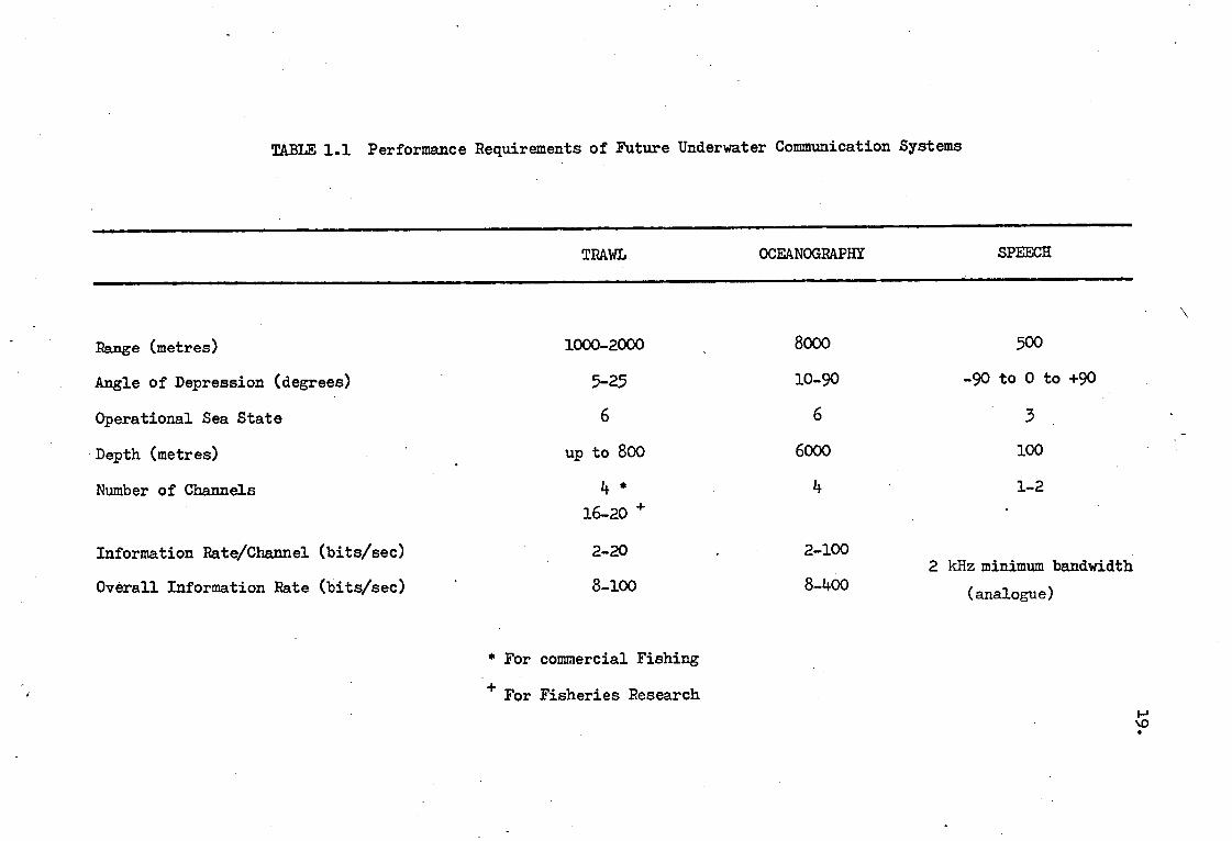
TABLE 1.1 Performance Requirements of Future Underwater Communication Systems

TRAWL OCEANOGRAPHY SPEECH

Range (metres) 1000-2000 8000 500

Angle of Depression (degrees) 5-25 10-90 -90 to 0 to +90

Operational Sea State 6 6 3

Depth (metres) up to 800 6000 100

Number of Channels 4* 4 1-2

16-20 +

Information Rate/Channel (bits/sec) 2-20 2-100 2 kHz minimum bandwidth

Overall Information Rate (bits/sec) 8-100 8-400 (analogue)

* For commercial Fishing

For Fisheries Research

20.

underwater speech and data transmission systems. The constraint of

shallow-water propagation introduces the effect's of boundary reflections

which result in multipath propagation and leads to a degradation in

system performance.

Early telemetry systems did not, in general, incorporate specific

designs to overcome signal degradation. A typical system is that

described by Hearn (1966). This telemetry system was used in a

fish-trawling application and was designed to transmit, from the trawl

net to the trawler, information concerning the 'mouth-spread' of the

net, the water temperature, the strain on the net, and the height of the

top of the net from the bottom of the ocean. This information was

time-multiplexed and transmitted to the trawler using a 40 kHz

transducer. The system was used in the situation in which the water

depth was approximately 500 metres and the total transmission path

length was of the order of 1500 metres. The data-rate of the system

was very slow, typically 60 data pulses per second, and the method

for reducing multipath interference was to assume that the direct-path

signal always preceded the multipath signals at the receiver.

Triggering circuits in the decoding section of the receiver were based

on the above assumption. Because of the low data-rate, sophisticated

techniquet for reducing multipath interference were not necessary, and

automatic gain control (AGC) was not used.

A few years later, and with the same application in mind, Goddard

(1970) and Nesbitt and Berktay (1971) developed two different telemetry

systems for use in the fish trawling situation. Because the desired data-rate

was much higher (2000 bits/sec) than in Hearn's system, techniques for

reducing the effects of multipath interference were implemented.

Goddard's system was based on a time-gating principle, in which data

21.

was transmitted for a duration less than the difference in time between

the arrival of the direct-path signal and the multipath signals. The

transmission was then stopped, until the multipath arrivals had ceased

and then transmission was resumed. When using a carrier frequency of

104 kHz, a data-rate of approximately 2000 bits per second was achieved

at a range of 300 metres. An automatic gain control system was built

into the receiver to overcome signal fluctuations.

The system developed by Nesbitt and Berktay (1971) was based on an

electronic tracking idea. Using the principle that the direct-path

signal always precedes any of its multipath signals at the receiver, the

beam pattern of the receiving transducer was deflected in the direction

of the direct-path signal. This provided an attenuation of the

multipath signals by the use of the receiving directivity response. In

the system, which operated at a carrier frequency of 89 kHz over a

range of about 250 metres, an alignment sequence was transmitted every

100 msec in order to effect the tracking operation. No indication of

the achieved, or desired data-rate was given in the paper.

A special, and very complicated, signalling format was used to

reduce multipath interference effects in the system developed by

Miller and Bohmann (1972). Thirty-two frequencies, in multiples of

68.4 Hz, centred at 7.0 kHz, were available to scramble the data bits.

The choice of frequency was based on a coding procedure and the

data-rate to be transmitted. Four parallel transmission channels,

ranging from 17.5 kHz to 42 kHz were available and the already

scrambled data bits were encoded into pairs and then transmitted using

FSK techniques over the parallel channels. This complicated frequency

diversity technique was used to transmit data at ranges up to 700

metres at a maximum data-rate of 1640 bits per second.

The principle is not generally true but it is valid in many situations.

22.

Another telemetry system, employing a time-gating principle

similar to that used by Goddard (1970), has been described by Okerlund

(1973). The system was tested at a range of 2000 metres, and data was

transmitted for a time interval less than the difference in transmission

time between the direct-path signal and the surface-reflected path

signal. The transmission was then stopped and resumed after the

multipath signals had ceased to exist at the receiver. The data-rate

achieved was about 3100 bits per second using a bandwidth of nearly

20 kHz centred at a carrier frequency of 50 kHz.

The systems which have been described appear to have functioned

well in the particular environments for which they were designed and

tested, but they are likely to be less effective in a more general

environment. For example, the time-gating principle, although very

effective under certain conditions, does have some limitations. As

the difference in transmission time between the direct-path signal

and the surface-reflected path signal changes (resulting from a change

in range or transducer depth), it becomes difficult to transmit data

at a constant rate. This arises from the fact that the time allowed

for the transmission of the data changes with changes in range or

transducer depth, and in order to maintain a constant data-rate, a.

change in'both the transmitter and receiver timing circuitry may be

necessary. This might not be possible in practice, and if the

difference in the propagation time between the direct-path and the

surface-path becomes small enough, then the system bandwidth could

limit the performance of the system. This particular problem can

arise in the case of long-range transmission.

Although the idea of frequency diversity may, at first sight,

seem to be an effective method for reducing multipath interference,

23.

it also has a limitation. The movement of the water surface causes a

Doppler frequency shift of a surface-reflected signal, and frequency

shifts of the order of 0.2% of the carrier frequency could be expected

under many conditions. At, say 100 kHz, this would mean a frequency

shift of about 200 Hz. Thus, for the effective reduction of multipath

interference using frequency diversity techniques with only one

transmission frequency, quite large frequency shifts would be required

in an FSK system. Also, as the data-rate is increased, the time

diversity would decrease accordingly, thereby losing the advantages of

the frequency diversity. The idea of using several parallel transmission

frequencies is attractive, but involves a much more complicated, and

costly, data transmission system.

There are also several other techniques which could be used to

reduce multipath interference effects and thereby achieve high data-rates.

One method, space diversity, offers an effective method of reducing the

effects of multipath, but this method can involve the implementation

of quite large and complex receivers. In the case of long-range

shallow-water propagation, it may become difficult to distinguish the

the direct-path from the multipaths in both time and space.

The use of matched filters to recover signals embedded in noise is

a well-known technique in radar systems. Tests, using this technique,

have been carried out in the underwater environment by Parvelescu and

Clay (1965). However, since multipath interference is usually a time-

varying phenomenon, matched filters are not often effective when

operating in a multipath environment.

In order to optimise the implementation of an underwater data

transmission system, many aspects relating to underwater data

transmission need to be investigated. At present, little is known

24.

about the manner in which data pulses fluctuate and how these fluctuations

affect the data-rate. The time-varying nature of multipath interference

has not been completely investigated nor have the achievable data-rates

and the related error probabilities for a particular underwater

environment and data transmission system. The purpose of this thesis is

to investigate some of these problems and thereby provide a clearer

understanding of some of the underlying factors which affect underwater

data transmission.

1.3 Aims and Outline of the Thesis

The maximum information capacity of an underwater communication

channel has been studied by Rowlands and Quinn (1967) using a simple

approach, and a more detailed and complicated approach has been

adopted by Marsh and Rowlands (1968). Although these theoretical

investigations present an indication of the maximum data-rate which can

be attained for a particular system bandwidth and signal-to-noise ratio,

present-day data transmission systems do not appear to approach these

theoretical limits.

Signal amplitude fluctuation is the main reason for the large

difference between the maximum theoretical and the actual practical

data-rates that have been achieved. These fluctuations originate from

three main sources - multipath interference, thermal inhomogeneities,

and background noise. The effect of signal amplitude fluctuations on

a data transmission system is to increase the probability of detection

error, which implies a subsequent limitation of the data-rate if

communication is to be carried out with a maximum prescribed

probability of bit-error.

Quantitative results relating to the effect of signal amplitude

fluctuations on system performance have not been widely reported.

25.

In particular, little has been reported on the effect of signal

amplitude pertubations on the bit-error probability of an underwater

data transmission system. There have, however, been several papers

which have reported on some general aspects of underwater acoustic

signal amplitude fluctuations.

A considerable body of literature exists on experimental

investigations of signal amplitude fluctuations arising from thermal

inhomogeneities ( Stone and Mintzer, 1965; Campanella and Favret, 1969;

and Sagar, 1973 ), and on signal amplitude and phase characteristics

determined over long propagation paths using low-freuency CW

transmissions ( MacKenzie, 1962; Steinberg and Birdsall, 1966; Nichols

and Young, 1968; and Stanford, 1974 ). Two other experimental works

( Whitmarsh et al, 1957; and Whitmarsh, 1963 ) have reported on various

aspects of signal amplitude fluctuations of both direct-path and

surface-reflected path signals. In all the above-mentioned

publications, little indication has been given as to the effect that the

signal amplitude fluctuations have on the performance of data

transmission, or sonar, systems.

The performance of a data transmission system can be evaluated in

several ways. An important parameter used to evaluate the performance

of a system is the bit-error probability. In order to predict

theoretically the bit-error probability of a particular system, it is

essential to have some knowledge of the probability density function

(PDF) of the received signal amplitude. Some experimental investigations

have been carried out to determine the signal PDF under a variety of

propagation conditions. The results have indicated that the received

signal PDF is quite variable ( MacKenzie; 1962 ) and can range from

Rayleigh and Gaussian distributions ( MacKenzie, 1962 ) to a Rician

26.

distribution Goddard, 1970 ). The fact that the nature of the PDF is

extremely variable and still relatively unknowh, suggests that more work

is needed on this important aspect. Although some work has been done to

evaluate bit-error probabilities for a particular system ( Abotteen et

al, 1974 ), it is necessary to know some of the characteristics of the

signal PDF in more detail. It is necessary, that this be done if the

effects of climatic and propagation conditions are to be adequately

taken into account. In this way, it may be possible to develop a more

detailed and specific model for use in the prediction of system

performance.

With many of the above-mentioned ideas in mind, a general programme

was undertaken to investigate several aspects relating underwater data

transmission. Specifically, the variation in performance of a

particular data transmission system was to be investigated. This would

involve an analysis of the effect of a variation of both climatic and

propagation conditions on the bit-error probability of the system.

Other factors, such as data-rate, data-pulse width, and the receiver

decision threshold, which might affect system performance, were also to

be investigated. An additional factor to be studied was the variation

in the signal amplitude characteristics under a variety of climatic

and propagation conditions. This included the determination of the

signal PDF and its related statistics. It was hoped that the information

obtained would be useful as an aid to a more general understanding of

the signal PDF, and as an aid in the development of more accurate

prediction models.

A prototype underwater data transmission system was designed and

tested. The system, which was based on the conventional amplitude-

shift-keyed (ASK) method of data transmission, was intended to provide

27.

some information about several aspects of underwater data transmission.

The reasons for the choice of ASK modulation over other forms of

modulation for the initial investigation can be summarised as follows:

1. with ASK, the demodulation process is simple and, at the start of

the work, very little information was available relating to the

problems of carrier extraction with systems operating in the water

medium;

2. with ASK, the pulse response of the overall system is more easily

understood and more easily interpretable because ASK modulation

and demodulation are linear operations;

3. as the provision of digital speech facilities is a likely possible

application of underwater data transmission, it seems reasonable

to expect that such systems will have to operate close to the

Nyquist transmission rate. Therefore, steps may need to be taken

to eliminate the effect of intersymbol interference arising from

pulse dispersion and multipath. One possible method of doing

this would be to use adaptive equalisation techniques and these

are much easier to apply to ASK systems than to PSK or FSK systems.

Because of the availability of only restricted range facilities

(less than 1.0 km), the system was designed to operate as a low-power

system, so that information relating to the limiting performance could

be obtained. Automatic gain control circuits were not used in the

prototype system since one of the main aims of the investigation was

to obtain information about the amplitude fluctuations of the received

signal.

In Chapter 2, a detailed description of the prototype ASK system

is given. Attention is first drawn to the choice of an appropriate

carrier frequency to use in the system, with specific reference to the

28.

restricted range facilities and other important factors which would

affect transmission. A description of all the components of the ASK

system is given and in particular, the design,construction, and testing

of the ultrasonic transducers are described. In the last part of

Chapter 2, a description is given of the method of evaluating system

performance. The testing procedure is explained, as are the techniques

used in the analysis of the experimental data.

Chapter 3 is devoted to a consideration of the amplitude

fluctuations of the received signal. A presentation and discussion of

results relating to specific aspects of the amplitude fluctuations are

given. Results of measured PDFs, signal spectra and signal

autocorrelation functions are presented and interpreted with reference

to some contemporary theories. Using the experimental results presented

in the chapter, two models of the signal PDF are proposed, based on

climatic conditions.

The presentation and discussion of results of tests relating to

the bit-error probability of the ASK system are given in Chapter 4.

The results are classified into two main categories in order to

interpret the performance of the system more easily. Using the PDF

models derived in Chapter 3, bit-error probabilities are predicted and

the results of the prediction are compared with experimentally

measured error probabilities. A derivation of the optimum fixed

detection threshold level is made from a consideration of the PDF

models proposed in Chapter 3. Values of the detection threshold level

are computed for a range of signal-to-noise ratios.

The baseband pulse response of the system is considered in Chapter

5. Some provisional experimental results are presented and these are

interpreted in terms of the propagation and climatic conditions under

29.

which they were measured. The work presented in this chapter is only

provisional and much remains to be done. A knowledge of the pulse

response, and the way in which it varies with time, is important in any

consideration relating to high-rate data transmission, and in any

possible application of techniques such as adaptive equalisation.

In Chapter 6, a summary of the work presented in the thesis is

given, and some general conclusions are drawn based on the results of

the investigation. Also, some suggestions for further research are made.

30. CHAPTER TWO

DESCRIPTION OF THE PROTOTYPE ASK DATA TRANSMISSION SYSTEM

AND DISCUSSION OF EXPERIMENTAL PROCEDURES

Introduction

In the first part of this chapter, some of the factors which

affect underwater acoustic propagation are considered. These factors

are then used to determine a suitable carrier frequency for an ASK

system for use at transmission ranges up to 1.0 km. A complete des-

cription of the ASK data transmission system is given. In the last

part of the chapter, an outline of the procedures used in the testing

of the system is provided and a description of the techniques used

in the analysis of the test data is presented.

2.1 Factors Affecting Underwater Acoustic Propagation

In this section of the chapter, some of the factors which affect

acoustic propagation are considered briefly. By making several, rather

general, assumptions about these factors, an upper limit for a suitable

carrier frequency is determined as a function of the desired receiver

signal-to-noisy ratio.

2.1.1 Spreading Loss

One of the fundamental losses encountered in underwater acoustic

propagation is the loss due to the divergence of the acoustic wave-

front as it propagates through the medium. In an unbounded medium, this

geometrical spreading is spherical, but in the case in which boundary

reflections are present, the spreading tends toward a cylindrical

divergence (see Tucker and Gazey, 1966). The spreading loss (SPL),

expressed in decibels, is

SPL = 10nlog (r) (relative to 1 metre) (2.1)

where r = range in metres, and

31.

n = 1 ; for cylindrical spreading

= 2.; for spherical spreading

2.1.2 Absorption Loss

On account of its non-ideal nature, the water medium absorbs

acoustic energy. The absorption losses of a propagating acoustic signal

are associated with effects such as viscosity, thermal conduction and,

in the case of sea-water, relaxation phenomena. For fresh-water, at

15°C, the absorption coefficient due to these effects is, (Kinsler and

Frey,1962),

al = (2.4 x 107)f2 dB/metre (2.2)

where f is the transmission frequency in kHz.

For sea-water, at 150C, the absorption coefficient is, (Kinsler

and Frey,1962),

a2 al 0.036f2

dB/metre (2.3)

f2 + 3600

The second term in equation (2.3) takes account of the increase in

acoustic absorption of sea-water at 60 kHz due to the dissociation

of dissolved magnesium sulphate. The manner with which the attenuation

coefficients, al and a2, vary as a function of frequency, is shown in

FIGURE 2.1. The absorption loss, ALT in terms of the absorption co-

efficients and the transmission range, is therefore,

AL = air . dB (2.4)

where i = 1 or 2, depending on whether propagation is in fresh-water

or sea-water, and r is the transmission range in metres.

1000

( KH Z )

10

FREQUENCY 100

.01

C) FRESH WATER

1.•

•001

•0001

2

SEA WATER

32.

FIGURE 2.1 Fresh-Water and Sea-Water Attenuation Coefficients

as a Function of Frequency

33- 2.1.3 Source Level and Transducer Gain

The source level, SL, is expressed in terms of the radiated

acoustic power and the gain due to the directivity of the transmitting

transducer.

The acoustic intensity of an omnidirectional source is

Wr SI = 10logioH 4n

= -11 + 101og10Wr dB (relative to 1 Watt/M2)

(referred to 1 metre) (2.5)

where Wr is the radiated source power in Watts.

To obtain an expression for the source level, SL, for a given source

intensity, SI , an additional gain factor has to be included on

account of the directivity' of the transducer. This gain factor (SD),

which is a function of the directivity index of the transducer, is

given by,

( 7cAs dB SD = 101og10 4 (2.6)

where As = area of the transmitting transducer and,

X = acoustic wavelength of the transmission frequency in

the medium.

On including this directivity factor, the source level, SL, of

the transmitter is seen to be,

SL = SI SD

dB (relative to 1 W/m2) (2.7)

Similarly, the receiver has a gain factor (RD) associated with

its directivity. This factor is,

14 RD = 10logio ( :1I..) dB

where Ar is the area of the receiving transducer.

(2.8)

34.

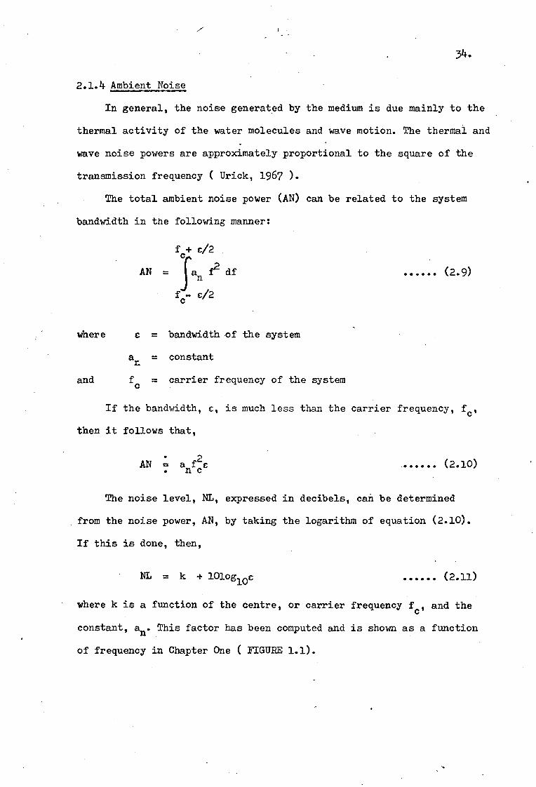
2.1.4 Ambient Noise

In general, the noise generated by the medium is due mainly to the

thermal activity of the water molecules and wave motion. The thermal and

wave noise powers are approximately proportional to the square of the

transmission frequency ( Urick, 1967 ).

The total ambient noise power (AN) can be related to the system

bandwidth in the following manner:

fc c/2

AN = an f2 df

fc- c/2

(2.9)

where e = bandwidth of the system

a_ = constant

and fc = carrier frequency of the system

If the bandwidth, c, is much less than the carrier frequency, fc,

then it follows that,

• AN = a f2c . n c (2.10)

The noise level, NL, expressed in decibels, can be determined

from the noise power, AN, by taking the logarithm of equation (2.10).

If this is done, then,

NL = k 10log1oc (2.11)

where k is a function of the centre, or carrier frequency fc, and the

constant, an. This factor has been computed and is shown as a function

of frequency in Chapter One ( FIGURE 1.1).

35.

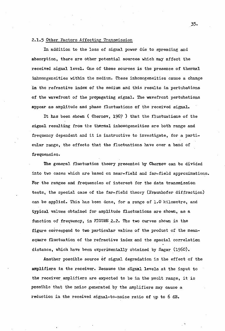
2.1.5 Other Factors Affecting Transmission

In addition to the loss of signal power due to spreading and

absorption, there are other potential sources which may affect the

received signal level. One of these sources is the presence of thermal

inhomogeneities within the medium. -These inhomogeneities cause a change

in the refractive index of the medium and this results in pertubations

of the wavefront of the propagating signal. The wavefront pertubations

appear as amplitude and phase fluctuations of the received signal.

It has been shown ( Chernov, 1967 ) that the fluctuations of the

signal resulting from the thermal inhomogeneities are both range and

frequency dependent and it is instructive to investigate, for a parti-

cular range, the effects that the fluctuations have over a band of

frequencies.

The general fluctuation theory presented by Chernov can be divided

into two cases which are based on near-field and far-field approximations.

For the ranges and frequencies of interest for the data transmission

tests, the special case of the far-field theory (Fraunhofer diffraction)

can be applied. This has been done, for a range of 1.0 kilometre, and

typical values obtained for amplitude fluctuations are shown, as a

function of frequency, in FIGURE 2.2. The two curves shown in the

figure correspond to two particular values of the product of the mean-

square fluctuation of the refractive index and the spacial correlation

distance, which have been experimentally obtained by Sagar (1960).

Another possible source Of signal degradation is the effect of the

amplifiers in the receiver. Because the Signal levels at the input to

the receiver amplifiers are expected to be in the Itvolt range, it is

possible that the noise generated by the amplifiers may cause a

reduction in the received signal-to-noise ratio of up to 6 dB.

100 1000 10

FLU

CT

UA

TIO

N

36.

FREQUENCY (KHz)

FIGURE 2.2 R.M.S. Amplitude Fluctuation Due to Thermal Inhomogeneities

37-

2.1.6 Derivation of the Maximum Transmission Frequency

By considering and taking account of the factors discussed above,

it is possible to estimate, for a desired signal-to-noise ratio at the

receiver, the maximum frequency which could be used for communicating

over a maximum range of, say, 1.0 kilometre. If a 'worst-case' approach

is adopted, then it is possible to provide a conservative estimate of

the transmission frequency. With the test site considerations in mind,

a worst-case analysis was in fact carried out for the situation in

which the desired range of communication was set at 1.0 kilometre. In

the analysis, the following assumptions and estimates of the system

parameters were made:

a) Spreading in the medium was assumed to be spherical.

b) A low transmitter power of 50 milli-Watts to be used.

c) The system bandwidth to be 10.0 kHz.

d) The directivity of the transducers will result in signal level

gains of 3 dB.

e) The ambient noise level is -120 dB relative to 1 Watt/m2.

f) Fresh-water absorption applies.

g) The transmitting and receiving transducers are identical.

h) Signal level fluctuations due to thermal inhomogeneities will be

of the order of 9 dB.

i) The receiver amplifiers result in a signal-to-noise ratio degradation

of 6 dB.( very pessimistic estimate)

Under the above assumptions, the maximum usable frequency, as a

function of the desired signal-to-noise ratio at the receiver, can be

computed by determining the maximum frequency for which the equation,

SL + RD - SPL - AL - NL - 9 - 6 = SNR (2.12)

is satisfied. In Equation (2.12), SNR is the desired signal-to-noise

38.

ratio at the detector.

If this is done, then the results are as Chown in TABLE 2.1. The

frequencies in the table are the estimated maximum transmission fre-

quencies which could be used at a range of 1.0 kilometre for the in-

dicated signal-to-noise ratios. It is important to note that the values

obtained provide a conservative indication of the possible transmission

frequencies because of the 'worst-case' approach used in the analysis.

TABLE 2.1

Estimation of Maximum Transthission Frequncies at 1.0 km.

SNR MAXIMUM FREQUENCY

20 dB 60 kHz

10 dB 220 kHz

0 dB 280 kHz

2.2 The Test Site

The tests were carried out at the King George VI reservoir at

Staines, and the facilities were made available by the Admiralty

Research Laboratory (ARL), Teddington. The reservoir is approximately

1500 metres long and 600 metres wide and its depth varied from 16

metres during the period from mid-June to mid-September, to 13 metres

from mid-September to November. The ARL raft at the reservoir provided

electrical power facilities and test ranges of 150, 200 and 650 metres.

A diagram of the basic dimensions of the test site is shown in FIGURE

2030

In order to centralise the majority of the test equipment and

thereby simplify experimentation,a feedback cable link was established, for

each test range, between the ARL raft and the receiver. In this way,

both the transmitted and received signals could be observed together.

Range 2 200 m.

Range 3 650 m.

Range I 150 M.

AR L RAFT

FIGURE 2.3 Test Site Dimensions

40.

2.3 ASK Data Transmission System

2.3.1 Transducers

There were two main reasons for the final choice of the transmission

frequency to be used in the ASK system. Firstly, as was shown in Section

2.1.6, the choice depends on the desired signal-to-noise ratio at the

receiver. From TABLE 2.1 it can be seen that frequencies varying from

60 kHz to 280 kHz would be suitable at a range of 1.0 kilometre. As the

maximum range at the test site was limited to 650 metres, it might be

thought that frequencies somewhat in excess of those given in TABLE 2.1

would be most suitable. For example, as the maximum range is 650 metres,

this indicates that a transmission frequency of the order of 250 kHz

would be suitable and thatthis would still allow for unpredicted losses

and would still pcvide a sufficiently large signal-to-noise ratio at

the receiver. However, a brief investigation into the availability of

transducers with resonant frequencies of approximately 250 kHz revealed

that transducers of this type were not readily available and could not

be constructed from available parts. For this reason, it was decided

to construct transducers using easily available electro-acoustic crystal

elements.

The particular crystal which was selected was a PZT-5A thickness

vibrating ceramic disc, resonant in the thickness mode at 150 kHz.

This crystal was readily available and inexpensive. Although the

resonant frequency of this particular crystal was somewhat below the

intended frequency of 250 kHz, the crystal provided some desirable

properties for the transducer beam pattern.

It is possible to reduce the effects of multipath interference

by using directional transducers. For example, a transducer which has

a narrow vertical response and a wide horizontal response can reduce

the effects of multipath interference arising from both surface and

41.

bottom reflections. One of the aims of the experimental investigation

was to study the effects of multipath interference on the received

signal. Thus, by using a circular disc which has a symmetrical direct-

ivity response about an axis perpendicular to the face of the disc,

multipath effects could be studied more easily. Another advantage of

the PZT-5A type of crystal is that, unlike many other types of lead-

zirconate-titanate compounds, the 5A-type material has a low mechanical

Q-factor. This means that quite large bandwidths can be obtained.

The diameter of the crystal is 31 mm, or approximately three times

the acoustic wavelength of 150 kHz sound in water. The corresponding 2

area of the crystal face results in a transducer gain of 10 logio,4n (3.)2X

2]dB

4X = 19.7 dB - but the beamwidth is not very narrow. The directional

response of the circular disc is given by ( Tucl7er and Gazey, 1966 ), as,

D(x) 2J, (x)

(2.13) x

where J1(x) = first Bessel function of x,

x = sine , X

X = acoustic wavelength,

d = diameter of the disc ,

and e = angle of observation.

Using the appropriate values in Equation (2.13), the beam pattern

of the disc was calculated and is shown in FIGURE 2.4. The 3-dB beam-

width of the main-lobe is seen to be -8o from the maximum response,

and the first side-lobes occur at ±30° from the point of the maximum

response. The computed intensity of these side-lobes is -14 dB relative

to the maximum intensity.

In order to maximise the power radiated from the transducer, an

aluminium casing was designed to load heavily one face of the crystal

FIGURE 2.4 Theoretical Beam Pattern of the 150 kHz Transducer

10

14"tkill II 1,14**44 300

tatt4,411 ott 11011,6 '01,farrt Oq relatIve tage

1+3.

whilst allowing the other face to radiate freely the acoustic energy

into the water. The aluminium casing was of a dimension such that it

formed a quarter-wave transformer which provided a large mechanical

load on the back face of the crystal. The mechanical load on the crystal

face which radiates into the water is simply that of the water, while

the load on the opposite crystal face is considerably larger. The loads,

expressed in terms of acoustic impedances, on either side of the

crystal are,

Zface 1 = Zwater

z2aluminium

(2.14)

face 2 - water

The ratio of the acoustic impedances on either side of the crystal is

approximately,

Zface 1 = 1

Zface 2 125

(2.15)

From equation (2.15), it would be expected that less than 1% of the

radiated acoustic energy would be 'back-radiated' into the water

through the aluminium casing. A full-scale drawing of the encapsulated

PZT-5A crystal is shown in FIGURE 2.5.

The experimental measurement of both the directional response

and the electrical equivalent circuit of each of the transducers was

performed under somewhat restrictive conditions. A large concrete and

glass water tank of dimensions 5.25m x 2.7m x 2.6m was used, and in

order to reduce reflections from the bottom and sides of the tank, it

was necessary to line some parts of the inside of the tank with

acoustic absorbing material. A measured directivity pattern of one of

PZT-5A Ceramic Disc

Aluminium Casing

Electrical Connections

Silicone Rubber Compound

44.

FIGURE 2.5 Cross-Section of 150 kHz Transducer

45.

the transducers is shown in FIGURE 2.6. On comparing the measured

response shown in FIGURE 2.6 with the theoretidal response given in

FIGURE 2.4, it is seen that there is considerable agreement between

the two. In particular, there is excellent agreement with respect to

the value of the 3-dB beamwidth of the main-lobe of the response. The

measured value of 16° is identical to the predicted value. Also, the

intensity of the first side-lobes with respect to the main-lobe was

measured to have values of between -12 dB and -14 dB, which compare

well with the theoretical value of -14 dB. There is, however, a dis-

crepency between the theoretical and practical values for the angle

between the maximum responses of the main-lobe and the first side-lobe.

The measured value of the angle was found to be ±230, whereas the

theoretical value is 130°. The difference is probably due to two main

causes..

A first possible cause of the discrepency between the measured

and theoretical angle is that the acoustic absorption of the tank was

not sufficient to prevent multipath interference effects from

occurring in the tank. A second possibility is that the bond between

the aluminium casing and the crystal was not uniform over the crystal

face, which could affect the radiating properties of the transducer.

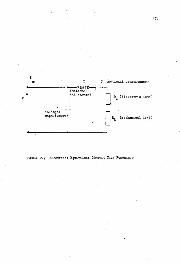
It is possible to obtain an electrical equivalent circuit for the

transducer by considering both the piezoelectric properties and the

physical dimensions of the crystal. Near to the main resonance of the

crystal, the transducer can be modelled by the R-L-C type circuit

shown in FIGURE 2.7. This particular form of the electrical equivalent

circuit of the transducer was derived mathematically by Mason (1948).

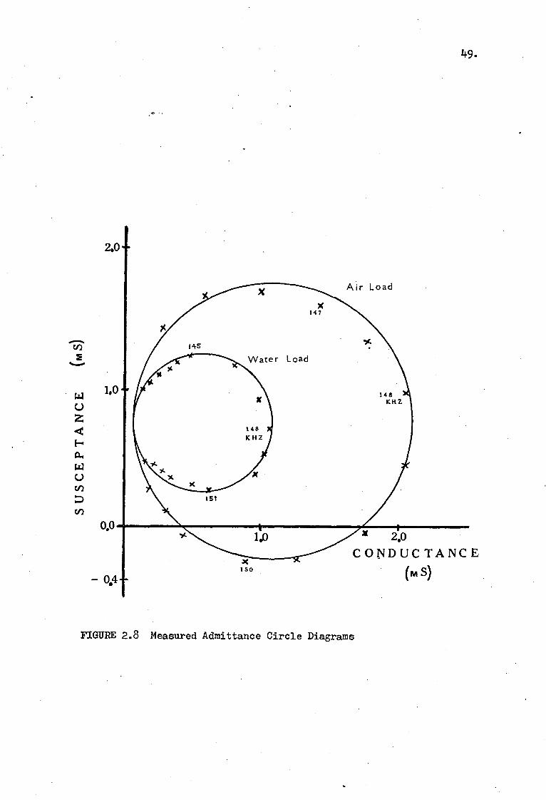
The measurement of the admittance of the transducer over a band

of frequencies near the mechanical resonance frequency makes it possible

0 •--Relative Voltage

FIGURE 2.6 Measured Directivity Pattern of the 150 kHz Transducer

1+7.

L C (motional capacitance)

Rd (dielectric loss)

(mechanical load)

0 (motional inductance)

Co (clamped capacitance)

FIGURE 2.7 Electrical Equivalent Circuit Near Resonance

1+8.

to determine values for the elements of the equivalent circuit. Using

frequency as a variable, a circle can be traced out on susceptance and

conductance coordinates. By computing two such circle diagrams, as

shown in FIGURE 2.8, for the cases of an air load and a water load on

the transducer, it is possible to compute values for the elements of

the equivalent circuit. A comparison of theoretical and actual computed

values from a consideration of the circle diagrams in FIGURE 2.8 is

shown in TABLE 2.2, from which it can be seen that the computed and

theoretical values are in good agreement.

TABLE 2.2

Comparison of Element Values

Element Theoretical Measured

Co 500 pF 600 pF

Rd 570 Q

L

25 mH 32 mH

C

30 pF 28 pF

The electro-acoustic efficiency of the transducer can also be

computed from a consideration of the admittance circle diagrams ( see

Tucker and Gazey, 1966 ). A value of 48% has been calculated from the

values of the circle diagrams shown in FIGURE 2.8. Another important

parameter which can be calculated from a consideration of the circle

diagrams is the bandwidth of the transducers. The information contained

in the measured circle diagrams indicated that the transducers had a

mechanical Q-factor of 22, which corresponds to a bandwidth of 6.5 kHz.

Under measurement at the test site, however, the 3-dB bandwidth was

determined to be 9.0 kHz, which indicated a Q of 16.5. No obvious

U) 2

S U

SC

EP

TA

NC

E 1,0

0,0 2,0

CONDUCTANCE 150

- 0,4

2.0

49.

FIGURE 2.8 Measured Admittance Circle Diagrams

50.

reason has been found which explains this discrepency.

Similar measurements to those described aboVe were carried out on

the two transducers and they were found to have similar electrical and

directional properties. For example, the resonant frequencies of the

two transducers were found to differ not more than 300 Hz.

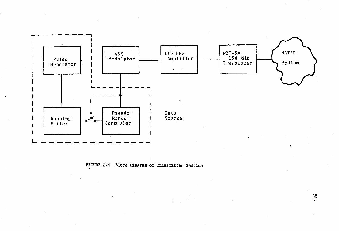
2.3.2 Transmitter Details

A block diagram of the transmitter section of the prototype ASK

data transmission system is shown in FIGURE 2.9. The data source consists

of a pulse generator, a shaping filter unit, and'a pseudo-random

scrambler. The pulse generator and shaping filter unit ( Andrews,

Constantinides and Turner, 1974 ), produces raised-cosine pulses with

100% roll-off. The raised-cosine frequency spectrum of the pulses is

given by,

H(w) = [1 + cos 2w (2a-il ; for twi 2w

c c (2.16)

= 0 ; elsewhere

where 2wc is the bandwidth of the pulse.

The pulse generator and shaping filter unit was designed to be

capable of generating a variety of data-pulse'widths and data-pulse

sequences. The pulse widths which can be generated are 0.8, 1.0, 1.6,

and 2.0 msec in duration. The unit is also capable of producing a large"

variety of repetitive 'on-off' pulse sequences and, by doing this, a

large number of data-rates, ranging from less than 250 bits/second to

1250 bits/second can be generated. The pseudo-random (PR) scrambler

can be either switched into operation or left out, as desired. The

generation of the PR sequences is based on the time-gating of .a

.1111=••

0-

.Pseudo- _.. .Alr Random

Scrambler

.111■. •■■■■ •ONNINEI ■•=1■1. ••■•••• 111I■••

-1

Data Source

_J

ASK Modulator

150 kHz Amplifier

PZT-5A 150 kHz

Transducer

L ■••■•■

Shaping Filter

FIGURE 2.9 Block Diagram of Transmitter Section

MINIM 4•■■ IMMMID •■■••

Pulse Generator

r

52.

continuous raised-cosine signal from the pulse generator unit, and the

resulting output is a PR sequence, of length (27-1) bits, of raised-

cosine pulses.

The ASK modulator is a commercially available unit which has a

variable depth-of-modulation facility. In the test system, a modulation

depth of 95% is used (rather than 100% for true ASK operation), so that

the simple and reliable demodulation scheme can be used in the receiver

(see Section 2.3.3). The modulator is then connected to a variable-power

amplifier which is used to drive the transmitting transducer. This

amplifier is capable of producing a peak-to-peak voltage of 50 volts

across the input terminals of the transmitting transducer. A simple

matching network, consisting of a single inductor, was used to resonate

with the static capacitance (Co) of the transducer. The transmitting

transducer has been described previously in Section 2.3.1.

2.3..3 Receiver Details

The receiver section of the ASK data transmission system is shown

in block diagram form in FIGURE 2.10. The acoustic signals are received

by the receiving transducer which is identical to the transmitting

transducer. The electrical signals from the output of the transducer

are then amplified by a line amplifier which is connected to an under-

water cable linking the receiver and transmitter. The received. signals

were transmitted back to the ARL raft over this cable. The line amplifier,

which is tuned to a centre frequency of 150 kHz with a pass-band of

±4.5 kHz about the centre frequency, is capable of providing a maximum

gain of 30 dB at the transmission frequency. By amplifying the signals

prior to transmission over the underwater cable, it was possible to

minimise effects such as cable noise and thereby prevent these effects

from causing a significant reduction in the signal-to-noise ratio of

BAND-PASS AMPLIFIER

HARD-LIMITER

COMPARATOR AND

ERROR COUNTER

TRANSMITTED SEQUENCE GENERATOR

1 VARIABLE

MULTIPLIER LOW-PASS THRESHOLD BIT 0• FILTER DETECTOR SYNCHRONISER

Analogue Digital Output Output

FIGURE 2.10 Block Diagram of Receiver Section

54. the signal during transmission from the receiving transducer to the

ARL raft.

During the tests, the signal received at the ARL raft was amplified

using a band-pass amplifier. This amplifier, which can provide a signal

gain variable up to 80 dB, has a bandwidth of ± 4.5 kHz centred at the

carrier frequency. The demodulation process, which may be considered as

a pseudo-synchronous form of detection ( Turner and Andrews, 1974 ),

provides a simple and reliable form of ASK demodulation. The detection

process consists of multiplying the band-pass version of the received

ASK signal by a hard-limited version of the same signal. The hard-limited

version is obtained by using a voltage comparator circuit which produces

an output in proportion to the zero-crossings of the received signal. As

mentioned previously, a 95% depth-of-modulation was used in the tests and

this made it possible to use the pseudo-synchronous detection scheme. On

account of the unwanted high-frequency components which are produced by

this form of detection, it is necessary to low-pass filter the signal

from the output of the detector. In the system, an active low-pass

Butterworth filter with a 4.5 kHz cut-off frequency is used. It is

important to note that the above detection scheme is the same as a full-

wave rectifier detector with a low-pass filter and hence the system used

in the ASK receiver operates as an envelope detector.

In order to perform tests capable of providing information about the

effect of the decision threshold level on the bit-error probability of the

ASK system, a variable threshold decision-making device was built into the

receiver. The device is essentially a voltage comparator, which compares

the incoming signal with a threshold voltage which can be altered easily.

Because of the relative movement of the transmitting and receiving

transducers arising from the motion of the rafts on the reservoir, it

was necessary to incorporate an adaptive timing circuit in the receiver.

55.

It was necessary to do this in order to ensure that corresponding digits in

transmitted and received sequences could be compared and a count of the number

of errors arising from transmission thereby obtained. A bit-synchronising

scheme, of the type described by Bennett and Davey (1965), was built into

the receiver. The sychroniser extracts timing information from the incoming

received bit-stream and uses this information to adjust the timing of a clock

generator in the receiver. This clock generator is then used in the

generation of a bit-sequence which is identical to the transmitted bit-

sequence. By doing this, timing differences between the transmitted and

received signals are overcome and a count of the number of errors

detected in transmission can be made.

A count of the number of errors detected in transmission was carried

out in the receiver. A sampling signal was generated from the receiver

clock using a monostable multi-vibrator. The sampling signal, which is

a 1.0 Ilsec duration pulse, is then used sample both the received and

transmitted data streams in synchronism. By using a simple 'exclusive-

OR' circuit and some additional logic, it was possible to compare the

two data sequences and to produce a pulse signal whenever the two signals.

differed. Thus, the number of errors ddtected in transmission could be

determined by simply counting the number of difference pulses. Both the

number of errors and the number of transmitted data pulses were counted

in order that information about the bit-error probability could be

obtained.

2.4 Test Procedures

The experimental testing of the ASK data transmission system was

divided into two groups. The first group of tests were carried out to

provide information about the amplitude fluctuations of the received

signal, and the second group of tests were carried out to provide

56.

information about the bit-error probability of the system. During the

course of the tests, detailed physical and cliMatic data were recorded

at the reservoir. The recorded data included the measurements of bathy-

thermographs (temperature-depth profiles), wind direction, air temperature,

and approximate wave heights and speeds. In all the tests, both the

transmitting and receiving transducers were, located at a depth of six

metres below the surface of the water.

2.4.1 Tests Relating to the Study of Signal Amplitude Fluctuations

The tests relating to the study of signal amplitude fluctuations

were carried out over a period of approximately twelve weeks, from mid-

June until mid-September, and were performed over transmission ranges

of 150, 200, and 650 metres. In order to obtain information relating

solely to the signal amplitude fluctuations, it is desirable, though

not essential, to eliminate intersymbol interference effects that result

from multipath propagation. It was found, after an initial investigation,

that intersymbol interference effects were negligible if data pulses

were transmitted at a rate of less than approximately 600 bits/second,

and it was decided, therefore, that if data pulses were transmitted

every 6.4 msec (or a rate of 156 bits/second), then intersymbol inter-

ference effects would be small. In the tests, two pulse widths of 0.8

and 1.6 msec were used. The pulses which were received at the ARL raft

were demodulated and recorded on a wide-band FM tape recorder. Each test

consisted of transmitting either a 1.6 or a 0.8 msec duration pulse

with the pulses modulating a 150 kHz carrier signal. The duration of

each test was approximately three minutes and the entire test was

recorded on tape. Several tests were carried out at each range under a

variety of climatic and propagation conditions. The peak signal-to-RMS

noise ratio was also measured at each test range.

57•

2.4.2 Tests Relating to the Study of Bit-Error Probabilities

As mentioned previously, there are three main sources of error in

underwater data transmission systems - multipath interference, thermal

inhomogeneities, and noise. The tests relating to the study of the bit-

error probabilities were designed to provide information about the

errors arising from these effects. In order to accomplish this objective,

it was necessary to vary a number of system parameters and to investigate

the effect of the variation on the bit-error probability.

The experimental investigation was carried out at all three test

ranges over a period of five months beginning in mid-June 1971+ and

ending in mid-November 1974. By performing the tests over such an

extensive period of time, any large changes in the prevailing climatic

conditions could be covered fully in the experimental investigation

and the results could be interpreted accordingly. In order to investigate

the effects of the various sources of error, three test parameters were

varied. The parameters varied were the data-rate, the data-pulse width,

and the detection threshold level. By varying these three parameters, it

was hoped that information relating to the way in which amplitude

fluctuations affect the performance of the ASK system could be obtained.

At each range, the fdllowing fixed test procedure was used:

1. A data signal was transmitted and the peak signal-to-PMS noise

ratio was measured. By doing this, it was possible to set the

detection threshold level as a fraction of the average peak

signal amplitude.

2. A pulse width was selected.

3. A data-rate was then set for the particular data pulse width.

4. Data was then transmitted and the number of errors detected in

transmission were counted. The total number of transmitted data

pulses for each test was set at approximately 300,000. This

58•

particular value was selected because a preliminary series of

tests had shown that error-rates of between 10-2 and 10-4

frequently occurred. A value of approximately 300,000 was

estimated to be sufficient to measure the short-term error

probability accurately. The duration of each test varied from

about four to twelve minutes, depending upon the data-rate.

5. A new data-rate was set and step 4 was repeated. In all, three

data-rates were transmitted for each pulse width.

6. A new pulse width was selected and steps 3 to 5 were repeated.

7. The detection threshold level was changed and steps 2 to 6 were

again carried out.

The above procedure was repeated many times at each test range over

the five month test interval. In total, several hundred short-term tests

were performed.

2.5 Data Analysis Techniques

2.5.1 Analysis of Tests Relating to the Study of Signal Amplitude

Fluctuations

Three bagic methods were used in the analysis of the tests relating

to the study of signal amplitude fluctuations. The first method of

analysis involved the computation of the probability density function

(PDF) of the signal amplitude. The PDFs were determined by analysing

the recorded data using a PDP-15 digital computer. The tape recordings

of the demodulated pulses were played into the analogue-to-digital (A/D)

converter of the computer and a programme was developed to sample the

pulses at the appropriate instances in time. The programme was such that

any number of samples could be taken and it was decided to carry out the

analysis by considering two sample sizes of 400 and 4000 data pulses,

which corresponded to respective time durations of 2.5 and 25 seconds.

59-

By doing this, both the long-term and short-term fluctuations could

be studied. In addition to computing the PDFs of the signal amplitude,

a programme was also developed to perform a statistical analysis of each

of the computed PDFs.

The statistics which were computed were based on the calculation

of the various moments of the probability distributions. The values

calculated were the mean (A), the standard deviation (6), the coefficient

of variation (V = VA), the skew and the kurtosis of the distribution.

These parameters were computed using the formulae,

A = 4:,x. N . 1=1

Xt

l=1

. - 5" b = ;:l

skew= --ILT i=1

N L-1 - Exl - 21 S- i=1V 1 + 2A31 A3

[I

N N

(2.17)

kurtosis = x. 4A N i=1

6A314 2 A 4 11 4 1=11

-17- - 7 ,- i=1

where. 3c3. .th = of data sample

N = number of samples

These formulae are standard and have been used previously by MacKenzie

(1962).

Two other parameters were determined when analysing the signal-plus-noise

amplitude fluctuations. The parameters computed were the amplitude

frequency spectra and the autocorrelation function of the signal-plus-noise

envelope. These parameters were determined in order to provide

information about the spectral distribution of the amplitude fluctuations

and about the rate of change of the fluctuations.

The tape recordings of the demodulated pulses were played into a

In the remaining part of the thesis, the word 'signal' refers to the signal-plus-noise unless otherwise stated.

60.

20 Hz sixth-order active low-pass filter. The resultant signal was then

fed into the A/D converter of the computer where it was sampled and

converted into a digital signal suitable for computer processing. A

programme based on the fast Fourier transform (rli) algorithm was

developed to compute the amplitude frequency spectrum of the data signal.

The autocorrelation function of the signal envelope was calculated by

first computing the amplitude frequency spectrum of the signal. The

spectrum was then squared, and the resultant signal, the power spectrum,

was inverse-transformed, using the FFT routine, back to the time domain.

This operation resulted in the formation of the autocorrelation function

of the signal envelope.

.2.5.2 Analysis of Tests Relating to the Study of Bit-Error Probabilities

The results of the several hundred 'short-term' tests relating to

the study of the bit-error probability of the ASK data transmission

system were used to compute 'long-term' or average bit-error

probabilities. This provided information about the average performance

of the ASK system.

During the testing of the system, three parameters were changed in

order to study the effect of their variation on the performance of the

system. These parameters were the data-pulse width, the data-rate, and

the detection threshold level in the receiver. Because four data-pulse

widths, three data-rates for each pulse width, and two detection

threshold levels were used in the tests at each range, then it was

possible to compute twenty-four average bit-error probabilities for

each range tested.

In the presentation of the results of tests relating to the study

of bit-error probabilities in Chapter lc, it will be shown that the

average bit-error probabilities can be further sub-divided into two

61.

groups which are related to the time of year during which the tests

were carried out. As will be shown in Chapter 4, it is possible, by

dividing the results in this way, to interpret them more easily and

more meaningfully in terms of the prevailing climatic conditions at

the test site.

62. CHAPTER THREE

A STUDY OF SIGNAL AMPLITUDE FLUCTUATIONS

Introduction

In this chapter, the amplitude fluctuations that result when pulses

are transmitted through water are considered, and several aspects

relating to these fluctuations are discussed. In particular, signal

amplitude probability density functions (PDF) and the statistics which

relate to the PDFs are examined. In addition, the signal envelope

frequency spectra and the envelope autocorrelation functions are

considered.

In the final part of the chapter, two models of the signal PDF are

developed. The models, which are based on the consideration of the

experimental investigation of the signal amplitude fluctuations, are

developed in terms of two prevailing wind directions.

3.1 Amplitude Fluctuations and Their Relevance to Underwater Data

Transmission

Signal level fluctuations can cause errors in the detection of

pulses transmitted through water. If the detrimental effects of pulse

amplitude fluctuations are to be overcome, then it is necessary to

have detailed information about the fluctuations. There are various

aspects of the amplitude fluctuations that are of importance in data

transmission. Firstly, the probability density function of the signal

amplitude is important since it provides information about the range

of the fluctuations and about the most likely amplitudes which the

signal can have. A knowledge of this information is useful when

studying the way in which the variation of the detection threshold

affects the error probability in a data transmission system.

There are two other aspects of amplitude fluctuations which can

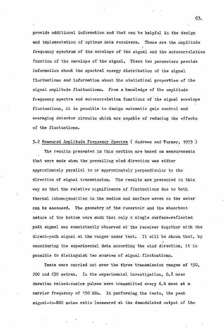
63.

provide additional information and that can be helpful in the design

and implementation of optimum data receivers. These are the amplitude

frequency spectrum of the envelope of the signal and the autocorrelation

function of the envelope of the signal. These two parameters provide

information about the spectral energy distribution of the signal

fluctuations and information about the statistical properties of the

signal amplitude fluctuations. From a knoWledge of the amplitude

frequency spectra and autocorrelation functions of the signal envelope

fluctuations, it is possible to design automatic gain control and

averaging detector circuits which are capable of reducing the effects

of the fluctuations.

3.2 Measured Amplitude Frequency Spectra ( Andrews and Turner, 1975 )

The results presented in this section are based on measurements

that were made when the prevailing wind direction was either

approximately parallel to or approximately perpendicular to the

direction of signal transmission. The results are presented in this

way so that the relative significance of fluctuations due to both

thermal inhomogeneities in the medium and surface waves on the water

can be assessed. The geometry of the reservoir and the absorbent

nature of the bottom were such that only a single surface-reflected

path signal was consistantly observed at the receiver together with the

direct-path signal at the ranges under test. It will be shown that, by

considering the experimental data according the wind direction, it is

possible to distinguish two sources of signal fluctuations.

Tests were carried out over the three transmission ranges of 150,

200 and 650 metres. In the experimental investigation, 0.8 msec

duration raised-cosine pulses were transmitted every 6.4 msec at a

carrier frequency of 150 kHz. In performing the tests, the peak

signal-to-RMS noise ratio (measured at the demodulated output of the

64.

receiver) was held at values of between 25 dB and 30 dB, depending

upon the transmission range. This was accomplished by increasing the

transmitter power as the range was increased. The received signal

was demodulated and recorded -on magnetic tape and the computation of

the amplitude frequency spectra was carried out using the methods

described previously in Section 2.5.1. The peak signal-to-RMS noise

ratio was measured at each transmission range and in defining this

parameter, 'peak signal' refers to only the signal and not the signal-

plus-noise.

Recently, Urick (1974) has compared, favourably, signal amplitude

fluctuation spectra in long range underwater transmissions with wave

spectra curves based on the theory described by Neumann and Pierson

(1966). Therefore, in the following presentation of experimentally

determined amplitude frequency spectra which were computed from data

measured under short-range transmission conditions, a similar comparison

is made on the basis of Urick's results.

Some typical amplitude frequency spectra obtained from measurements

made under the condition of a prevailing parallel-wind are shown in

FIGURES 3.1 to 3.3, and corresponding perpendicular-wind spectra are

illustrated in FIGURES 3.4 to 3.6. In each of the figures, the RMS noise

voltage (measured in a 4.5 kHz band and normalised to the peak of the

fluctuation spectrum) and the approximate noise spectrum are also indicated.

Additionally, amplitude wave frequency spectra computed using a formula

derived by Marsh et al (1961) are shown in the figures. The wave spectra

curves were computed using Marsh's equation in the form,

A(w) = c

exp(-g2/w2s2) (3.1)

where c = constant

w = angular frequency

or a discussion and derivation of the noise spectrum level, see

APPENDIX D.

FREQUENCY (HZ) 4.0 B.0 12.0 16.0 20.0

I

0.0

-10.0

-20.0 s„

rz■ E -30'0 1-4

Cxltil -40.0 1-4

Eqn. (3.1) with s 55 cm/sec

Approximate Average

RMS Noise Voltage Measured in a 4.5 kHz. Band ( normalised )

- 50-0 S = 55 cm/sec

Noise Spectrum

— 64.0

FIGURE 3.1 Measured Amplitude Frequency Spectrum at 150 metres with a Parallel-Wind Condition

4.0 20.0 16.0 FREQUENCY (HZ)

8.0 12.0 0.0

PT 0 \ Eqn. (3.1) with s = 40 cm/sec

-10.0 -

Approximate Average SA,_x

a, -20.0 -4-

-30.0 I

RMS Noise Voltage Measured in a 4.5 kHz Band (normalised)

I S. 40 cm/sec -40'0-0 .


- 50.0 - Noise Spectrum

- 60.0

Sdc

-10-0 Approximate Average

FREQUENCY (HZ)

8.0 4.0 16.0 12.0 20 .0

- 52.0

0.0

Eqn. (3.1) with s = 35 cm/sec

I

- 40.0 S= 35 cm sec


z

/ Noise Spectrum


FREQUENCY (HZ)

4.0 0.0

8.0 20-0 4

12.0 16.0


-10.0

Approximate Average 14 54,x

-20.0

1-1 a,

,a14 -30.0

1

z -40.0— 1

6„0

-50.0

0

i S = 45 cm/sec


Noise Spectrum

FIGURE 3.4 Measured Amplitude Frequency Spectrum at 150 metres with a Perpendicular-Wind Condition

0.0

—10.0 Sd

-20.0

cf)

E -30.0 •

FREQUENCY (HZ)

8!0 16.0 20.0 I I

12.0

S= 35 cm sec • RMS Noise Voltage Measured in a

4.5 kHz Band (normalised) -40.


Noise Spectrum.

- 56. 0


Approximate Average

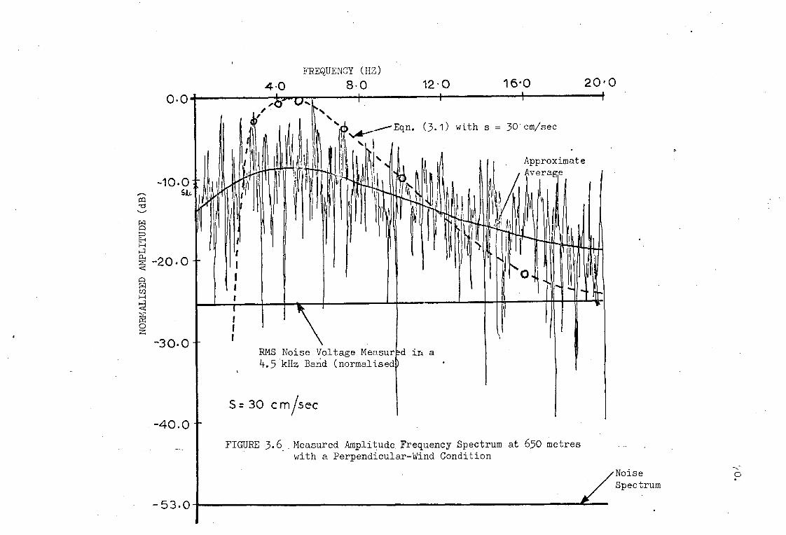
FREQUENCY (HZ)

4.0 8.0 20'0 16.0 12.0

-10.0 -3 (2

0.0


-20.0

It

-30.0 RMS Noise Voltage Measured in a 4.5 kHz Band (normalised

S=30 c misec -40.0


NOR

MAL

ISED

AMPL

ITU

DE

/Noise Spectrum

-53.0

Approximate Average

g = acceleration due to gravity 71.

and s = wind speed

The values of s which are indicated in each of the figures correspond

to experimentally measured wave speeds, rather"than to measured wind

velocities.

An examination of FIGURES 3.1 to 3.3 shows that there is similarity

between the experimentally determined amplitude frequency spectra and

the wave frequency spectra computed from Equation (3.1). The results

shown support the earlier results obtained by Urick (1974) and indicate

that in the case of a prevailing parallel-wind, there is similarity

between wave frequency spectra and amplitude frequency spectra.

The rapid fluctuations of the measured amplitude frequency spectra

shown in FIGURES 3.1 to 3.3 can be explained in two ways. Firstly,

the amplitude frequency spectra were determined from a single 512-bit

time sample of data and the data sample was converted to its frequency

domain representation by using a fast Fourier transform algorithm in

which no averaging methods were used. Hence, the computed spectra are

only estimates of the actual spectra and contain inherent fluctuations

(see Oppenheim and Shafer, 1975 and APPENDIX B for a simple illustration).

In order to reduce the fluctuations caused by a finite-length time

sample of data, it would be necessary to use ensemble averaging

techniques such as Bartlett's procedure (see Oppenheim and Shafer,. 1975).

However, in each of the figures, an approximate 'average' line has been

drawn through the fluctuating spectra rather than using ensemble

averaging.

A second explanation for the fluctuations in the measured amplitude

frequency spectra when compared to the wave spectra given by Equation

(3.1) is the limitation of the wave spectra model in the case of the

experimental conditions encountered at the reservoir. The wave spectra

model is derived under the condition of a fully developed open sea in

72.

which there are asssumed to be an infinite number of simple harmonic

progressive waves all travelling in the same direction on the water

surface ( Neumann and Pierson, 1966 ). This assumption is less valid

in the case of a small bounded reservoir and hence, the actual spectra

of the surface waves on the reservoir could be discrete, rather than

continuous. When the fast Fourier transform of the amplitude

fluctuations of the signal envelope is computed, therefore, it is

possible to encounter frequencies in the spectrum at which there is

little spectral energy caused by the effect of the surface waves. On

conversion to a decibel scale, the small amounts of spectral energy at

these frequencies would appear as large negative spikes or troughs,

as illustrated in the figures.

From an analysis of FIGURES 3.1 to 3.3, the main difference between

the measured amplitude frequency spectra and the computed wave spectra

occurs in the frequency band below about 1 Hz. It is likely that this

difference can be attributed partly to noise, partly to fluctuations

arising from thermal inhomogeneities in the medium, and partly to slow

movements of both the transmitting and receiving platforms.

In the perpendicular-wind case, as illustrated by FIGURES 3.4 to 3.6,

the measured amplitude frequency spectra are more variable than in the

parallel-wind case, and although the resemblance to the wave spectra

phenomenon is still apparent, it is much less marked. It is conjectured

that, in the case of a wind which is perpendicular to the line of

signal transmission, the main cause of the signal amplitude fluctuations

is the presence of thermal inhomogeneities in the medium. It will be

shown later, in Section 3.4, that this conjecture is to some extent

substantiated by values obtained for the coefficient of variation of

the signal amplitude fluctuations.

73.

3.3 Measured Autocorrelation Functions ( Andrews and Turner, 1975 )

The autocorrelation functions which are presented in this section

were determined by using the.methods outlined previously in Sections

2.4.1 and 2.5.1. Some typical autocorrelation functions computed

from data obtained under the condition of a prevailing parallel-wind

are shown in FIGURES 3.7 to 3.9. The figures relate, respectively,

to transmission ranges of 150, 200 and 650 metres.

The autocorrelation functions shown in FIGURES 3.7 to 3.9 appear

to resemble the form of the exponential-cosine autocorrelation function.

This particular type of autocorrelation function is frequently

encountered in many applications ( Bendat, 1958 ), and the time of

occurrance of the second zero-crossing of the autocorrelation function

is indicative of a predominant frequency of the power spectrum of the

autocorrelation function ( Bendat, 1958 ). A more detailed discussion

is given in APPENDIX C. In the case of FIGURES 3.7 to 3.9, the time

of the second zero-crossing of the autocorrelation functions ranges

from approximately 0.2 to 0.5 seconds, which corresponds to predominant

frequencies of between 1.4 and 4 Hz (see APPENDIX C). These particular

values are in agreement with the peaks of the amplitude frequency

spectra shown in FIGURES 3.1 to 3.3, and thus, there is further

indication that in the parallel-wind case, the time-varying nature of

the pulse amplitudes is dependent strongly upon the effect of the

surface-reflected path signal. A conclusion which can be drawn from

the information contained in FIGURES 3.7 to 3.9 is that the statsitical

properties of the signal amplitude fluctuations can change at rates

of between about 1.4 and 4 Hz.

In addition to computing the autocorrelation functions for the

parallel-wind case, autocorrelation functions were also computed for

the perpendicular-wind case. It was found that, in general, when

-0.3 TIME (seconds)

NO

RM

AL

ISED

AM

PLI

TUD

E

1.0

0.9

0.6

0.3

0.0

0.3 0.6 0.9 1.2 1.5

FIGURE 3.7 Computed Autocorrelation Function at 150 metres with a Parallel-Wind Condition

1.0

0.9

NO

RM

ALI

SED

AM

PLIT

UDE

0.6

w vv 0.3 0.6 09 1.2 1.5

TIME (seconds)

0.3

0.0 I 411

-0.3 FIGURE 3.8 Computed Autocorrelation Function at 200 metres with a Parallel-Wind Condition

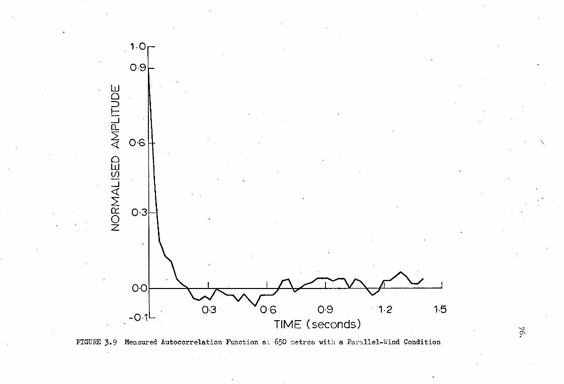
NO

RM

ALI

SE

D AM

PLIT

UD

E

0.6

0.3

0.0

1.5 0.3 0.6 0.9 1.2 TIME (seconds)

-0.1

1.0

0-9

FIGURE 3.9 Measured Autocorrelation Function at 650 metres with a Parallel-Wind Condition

1-0

0-9

0-6

0.3

0-0

0.1

NO

RM

ALI

SE

D AM

PLIT

UD

E

TIME (seconds)

FIGURE 3.10 Computed Autocorrelation FUnction at 650 metres with a Perpendicular-Wind Condition

78.

operating under perpendicular-wind 'conditions, the autocorrelation

functions are more variable than in the parallel-wind case. This

observation is to be expected from the fact that the apparent

dependence of the received signal on the surface-reflected path

signal is considerably less in the perpendicular-wind case than in

the parallel-wind case. In order to investigate the autocorrelation

functions for the perpendicular-wind case, a 30-second sample of

data was analysed. By doing this, longer term fluctuations could

be studied. A typical autocorrelation function for the perpendicular-

wind condition at a range of 650 metres is shown in FIGURE 3.10.

From this figure, it can be seen that beyond about 0.7 seconds,

there is little correlation of the signal. The results appear to

indicate that, although the dependence of the amplitude fluctuations

on the surface-reflected path signal is reduced in the perpendicular-

wind case when compared to the parallel-wind case, there is still

a concentration of spectral energy in the frequency band around 2 Hz.

This concentration of energy, which is mainly due to the surface-wave

effect, still has a considerable effect on the autocorrelation

function and on the statistical properties of the received signal.

3.4 Coefficient of Variation of the Amplitude Fluctuations ( Andrews

and Turner, 1975 )

From the point of view of pulse detection in data transmission

systems, the coefficient of variation, which is defined as the ratio

of the standard deviation to the mean of the function, is a highly

important parameter. The coefficient of variation was determined by

analysing the computed probability density functions of the signal

amplitude. The PDF's were computed, with the aid of a PDP-15 digital

79.

computer, using the techniques described in Section 2.5.1. The data-

pulse width used in the tests was 1.6 msec and two time sample lengths,

of 2.5 seconds and 25.0 seconds containing 400 and 4000 data samples

respectively, were used in the computation of the PDFs. The coefficients

of variation presented in this section are average values obtained by

taking account of more than 100 PDFs measured under the condition of

an approximate constant peak signal-to-RMS noise ratio at the output

of the receiver at all test ranges.

FIGURE 3.11, for example, shows the average coefficient of variation

of 2.5 second and 25.0 second data sample lengths at the three test

ranges for a wind which was perpendicular to the direction of signal

transmission. The measured RMS noise level, normalised to the mean

signal, is also indicated in the figure to illustrate the effect of

the background noise on the experimental results. Because the results

shown in FIGURE 3.11 are those obtained for the coefficient of variation

of the signal-plus-noise, two additional modified curves have also

been drawn in the figure. These latter curves refer to the signal-

only case. It can be observed that at the short ranges (less than

about 400 metres), the effect of the background noise is significant,

particularly in the case of the 2.5 second samples. The effect of the

noise is to reduce the values obtained for the signal-plus-noise case

to those shown for the signal-only case as illustrated in the figure.

Also plotted in FIGURE 3.11 are two theoretical curves derived

using the thermal fluctuation theory of Chernov ( 1967 ) with spacial

correlation distances of 0.5 metres and 1.5 metres. The equation from

which the theoretical curves were computed„ was,

DV n1 = [—ifccd k 2

(3.2)

1.0 100 150 200

RANGE (metres)

400 650 800

20.0

10.0

8.0

fa, 4-4 0

80.

RMS Noise Normalised to Mean Signal

-- X 25 Second Samples - Signal Plus Noise

25 Second Samples - Signal Only

O 4) 2.5 Second Samples - Signal Plus Noise

' 0-0 2.5 Second Samples - Signal Only

FIGURE 3.11 Average Coefficient of Variation For the Perpendicular-Wind Condition

81.

where, AV = RMS amplitude fluctuation (coefficient of variation)

—2 = mean-square fluctAation of the refractive index of water = 5.0 x 10-7

a = spacial correlation distance

R = range

k = 2n/X = acoustic wavenumber

X = acoustic wavelength in water

Equation (3.2) is derived from the general theory presented by Chernov

( 1967 ) under the assumption that the wave parameter, D, is large,

and where D is defined as,

D = 4nR

ka2

(3.3)

From an analysis of FIGURE 3.11, it is clear that the measured

coefficients of variation are in agreement with the RMS fluctuations

predicted from Equation (3.2) . The difference between the experimental

data and the two theoretical curves can be explained by the influence

of the effect of the surface waves, even under the perpendicular-wind

condition. The correlation distances used (0.5 and.1.5 metres) in

the predicted curves are in agreement with those which would be expected

from the theory of Tatarski ( 1967 ). The 25.0 second data shows

a larger coefficient of variation than the corresponding 2.5 second

data. This is to be expected since the longer time-samples include

longer term fluctuations of the signal, and the coefficient of variation

of the larger sample population should be greater than that of the

smaller samples of the same data.

FIGURE 3.12 shows comparative results for a wind parallel to the

line of transmission. The RMS noise level, normalised to the peak signal,

is also indicated but is not of significance to the measured results.

Because signal fluctuations due to both thermal inhomogeneities and the

RMS Noise Normalised to MeaA. Signal

82.

1.0 100

200

0 0

z0 10.0

< 8.0

• C _J LL t3 111 0

> D

▪ 0

40

- a) • U

8 ▪ 2.0

150 200 400 6508001000 RANGE (metres)

FIGURE 3.12 Average Coefficient of Variation for the Parallel-Wind Condition

20.0

0 0

Z 10.0

8.0

tL

0 4.0

CL

v).

GE 2.0

650 800 1000 1.0

100 150 200 400 RANGE (metres)

x---x---x 25.0 second samples 0--0 0 2.5 second samples

RMS Noise Level Normalised to rilekr1 Signal

FIGURE 3.13 Average Coefficient of Variation of the Surface-Reflected

Path Signal

84.

the effect of surface waves are caused by two different phenomena,

it is possible that these two sources can be considered statistically

independent and separable. The separation of the two sources of

fluctuations is based on the assumption that in the case of a

perpendicular-wind, the fluctuations are caused, in the main, by

thermal inhomogeneities in the medium. In the parallel-wind case,

however, the signal amplitude fluctuations will be caused by both

thermal inhomogeneities and the effect of surface waves ( the noise

is ignored in this case ). Then, if this is true,

-2 lw

= Vs + Vti

(3.4 )

and 17 - . 112 pw ti

(3.5)

where Tew = parallel-wind coefficient of variation squared

( mean-square amplitude fluctuation )

T/2 s = mean-square fluctuations due to the moving water surface

-2 Vti = mean-square fluctuations due to thermal inhomogeneities

. perpendicular-wind mean-square amplitude fluctuations Pw

By consideration of FIGURES 3.11 and 3.12, and -by using Equations

(3.4) and (3.5), it is possible to calculate the coefficient of

variation of the amplitude fluctuations caused by the moving water

surface only. This has been done and the results are shown in FIGURE

3.13. The RMS noise level, normalised to the peak signal is also

indicated in the figure. From FIGURE 3.13, it can be seen that the

fluctuations due to the movement of waves on the water surface tends

85.

to decrease with increasing range. This decrease with increasing

range appears reasonable since the grazing angle of the signal

incident on the water surface decreases as the range is increased,

and the undulating nature of the surface thus tends to have a reduced

effect on the incident signal as the grazing angle is decreased.

The results shown in FIGURE 3.13 are in agreement with results

obtained by Whitmarsh et al. ( 1957 ), although Whitmarsh's results

were obtained at a much lower transmission frequency.

The main conclusion which can be drawn from the results contained

in FIGURES 3.11 to 3.13 is that it appears that the effects of thermal

inhomogeneities and surface waves on the signal amplitude fluctuations

can be separated by using the simple technique of analysing the data

in the basis of parallel-wind and perpendicular-wind experimental

conditions. It will be shown in the following sections that because

of the apparent large differences between the parallel-wind and

perpendicular-wind data, it will be useful to develope PDF models

based on these two different wind directions.

3.5 Analysis of the Signal Probability Density Functions

The results presented in this section are given in terms of

86.

measurements made when the prevailing wind direction was approximately

parallel to and approximately perpendicular to the direction of

transmission. The results are presented in this way so that the effects

of thermal inhomogeneities and of surface waves on the signal PDF can

be observed. With the results of the previous section in mind, it was

felt that the analysis of the PDFsaccording.to the wind direction may

reveal properties of the PDF which are not easily observable on a more

general wind-direction basis.

The PDFs were determined from the analysis of demodulated 1.6 msec

raised-cosine pulses. Two sample lengths, of 2.5 seconds and 25.0

seconds in duration, were analysed using the techniques described in

Section 2.5.1.

At the 150-metre transmission range, the direction of the

prevailing wind was found to have a considerable effect on the

probability density function. This is illustrated in FIGURES 3.14 to

3.16. The PDF shown in FIGURE 3.14 was computed from data recorded

when the prevailing wind direction was approximately perpendicular to

the transmission path, while FIGURE 3.15 shows a comparative PDF under

the parallel-wind condition. An approximate intermediate value between

the parallel and perpendicular wind conditions is shown in FIGURE 3.16.

A point to be noted immediately from the three figures is that as the

prevailing wind changes from the perpendicular direction to the

parallel direction, the skew of the resultralt PDFs increase. This

observation can be explained by the consideration of two important

parameters.

Firstly, as shown in FIGURES 3.12 and 3.13, in the parallel-wind

case, the fluctuations of the signal amplitude are mainly dependent on

the effect of surface waves. Also, the effect of the surface waves is

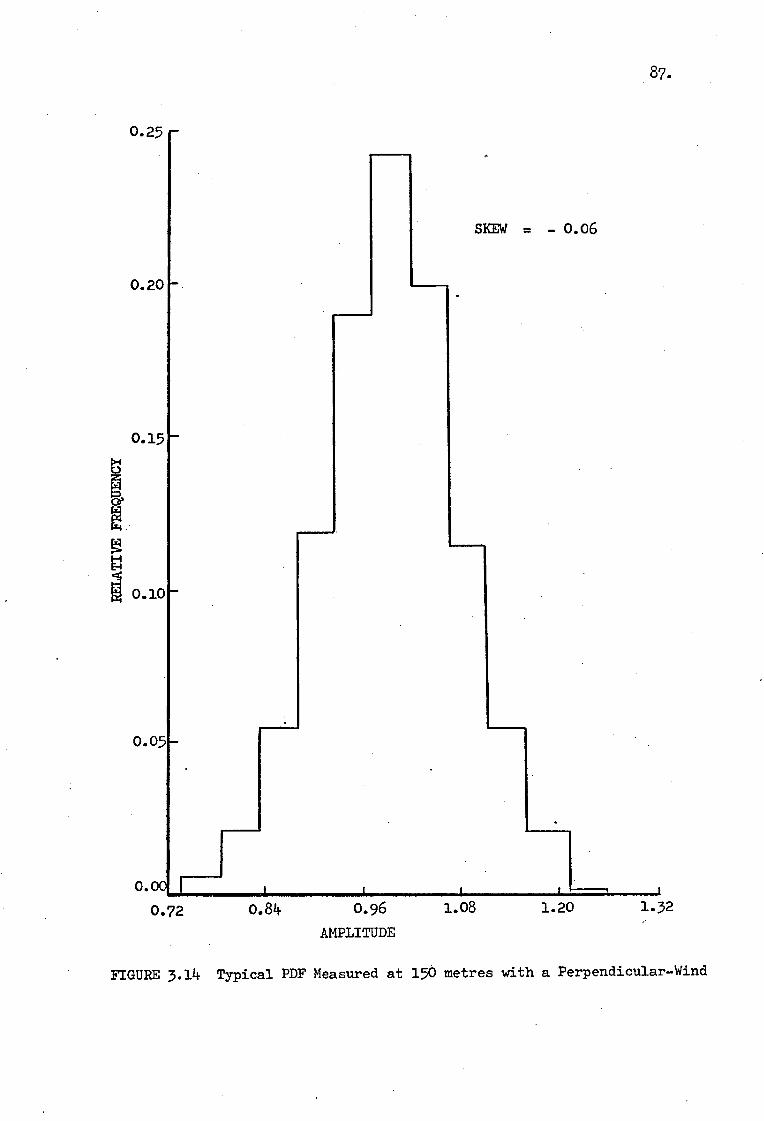
0.25

87.

0.20

0.05

1.08 0.00.j

0.72 0.84 1.20 1.32 0.96

AMPLITUDE

SKEW = - 0.06

FIGURE 3.14 Typical PDF Measured at 150 metres with a Perpendicular-Wind

88..

0.25

0.20 SKEW = 0.49

0.15 ,Iplow■■•••■•■•••

I

0.10

0.05

0.00 0.4 0.6 0.8 1.0 1.2 1.4

AMPLITUDE

FIGURE 3.15 Typical PDF Measured at 150 metres with a Parallel-Wind

0.25

0.20

89.

SKEW = - 0.11

0.15

0.05

0.90 0.00

0.78 1.02 1.14 AMPLITUDE

1.26 1.38

FIGURE 3.16 Typical PDF Measured at 150 metres - Intermediate Wind Direction

90.

0.20F

0.16 SKEW = 0.56

0.12

0.08

0.04

0.00 I I 0.5 0.6 0.7 0.8 0.9 1.0

AMPLITUDE

FIGURE 3.17 Typical PDF Measured at 150 metres under an Up-Wind Condition

91.

strongest at the shorter ranges because the undulating nature of the

surface has a particularly pronounced effect when the grazing angle is

largest. This is a situation. which occurs in the case of the 150-metre

range. The second important fact which appears to be of value in

explaining the results presented in FIGURES 3.14 to 3.16 is the effect

of the slopes of the surface waves on the signal reflected from the

water surface.

It has been shown ( Medwin, 1967 ) that the specular scattering

from the water surface is dependent mainly on the mean-square slope

of the surface waves. A down-wind parallel to the direction of

transmission can cause the mean-square slope of the surface waves to

become negative. This phenomenon will therefore cause the PDF of the

surface-reflected signal to become negatively skewed. Since the effect

of the surface-reflected signal on the received signal PDF is strongest

under the parallel-wind condition, it is to be expected that the largest

skew should occur in the parallel-wind case. This has been observed

at the 150-metre range, as illustrated by FIGURE 3.15. In the light of

the above and a consideration of the information contained in FIGURES

3.12 and 3.13, it might be expected that the skew of the parallel-wind

PDF should decrease with increasing range.

Although the results presented in FIGURES 3.14-to 3.16 apply to

the down-wind propagation direction, it is possible, from the mean-square

slope theory, to have a positive skew. A positive skew will result

when signals are propagated under up-wind conditions. An experimentally

measured PDF which illustrates a positive skew is shown in FIGURE 3.17.

Overall, it is probably reasonable to assume that the long-term, or

average, skew obtained under both up-wind and down-wind conditions

would tend toward a value of approximately zero.

92.

The statistical analysis of the computed probability density

functions can provide further information about fluctuations of the

received signal. The average statistics calculated from both

perpendicular-wind and parallel-wind PDFs are listed in TABLES 3.1 and

3.2 respectively. The values given in the tables were obtained by

finding the average value of the various parameters relating to more

than fifteen PDFs at each range, for two data samples of 2.5 seconds and

25.0 seconds duration. An examination of the tables reveals several

interesting trends.

The coefficient of variation, V, is always larger in the case of

a parallel-wind than in the case of a perpendicular-wind, for all test

ranges. Further information about the coefficient of variation can be

found in the previous section. The skew and the kurtosis (amount of

peakness) of the parallel-wind data are larger than those in the

perpendicular-wind case, and the skew tends to decrease with increasing

range. The latter observation is in agreement with the arguments

presented earlier in this section.

Fom the tables, it can be seen that the skew, in the parallel-wind

case, is positive, and not zero as conjectured previously. This can be

explained simply in terms of the prevailing climatic conditions at the

reservoir during the tests. It was found that the majority of the

experimental results were obtained under up-wind propagation conditions,

and this can almost certainly account for the positive skews shown in

TABLE 3.2.

3.6 Derivation of Probability Density Function Models

The material of Sections 3.2 to 3.4 shows that when short-duration

sound pulses are transmitted under shallow-water conditions the

amplitude fluctuations of the pulses are related to the direction

93.

TABLE 3.1

Perpendicular-Wind Statistics

2.5 Second Samples

RANGE

25.0 Second Samples

RANGE V SKEW KURTOSIS V SKEW KURTOSIS

150m. 0.05 +0.17 2.81 150m. 0.07 +0.06 2.47

200m. 0.06 -0.05 2.80 200m. 0.08 -0.17 2.63

650m. 0.10 +0.07 2.65 650m. 0.13 +0.03 2.62

TABLE 3.2

Parallel-Wind Statistics

2.5 Second Samples 25.0 Second Samples

RANGE V SKEW KURTOSIS RANGE V SKEW KURTOSIS

150m. 0.14 +0.21 3.16 150m. 0.18 +0.41 2.45

200m. 0.11 +0.26 3.02 200m. 0.16 +0.20 2.71

650m. 0.14 +0.11 2.85 650m. 0.16 +0.08 2.83

94.

of the prevailing surface wind. This suggests that the probability

density functions might also depend on the wind direction and, further,

that it might be possible to obtain theoretical models for the PDFs.

that are functions of wind direction. In order to test this hypothesis,

a series of experiments were performed in which 0.8 msec duration

raised-cosine pulses were transmitted under shallow-water conditions.

The transmitter and receiver of the system were located so that the

received signal was comprised of the direct-path signal and a single ,

essentially non-overlapping surface-reflected path signal. In setting

up the system, care was taken in positioning the receiver to ensure

that a minimum of interference occurred between the direct and surface-

reflected path signals.

Using the test system, the PDFs of the envelopes of the direct-

path and surface-reflected-path signals were measured for both

perpendicular and parallel-wind conditions, and typical results are

shown in FIGURES 3.18 and 3.19. Although FIGURES 3.18 and 3.19 show

some 'within curve' fluctuation caused by the coarseness of the

quantisation of the signal amplitude range, a comparison of FIGURES

3.18b and 3.19b shows that there is a considerable difference between

the PDFs of the envelopes of the surface-reflected-path signals for the

two different wind conditions. Under the perpendicular-wind condition,

the PDF of the signal envelope appears to resemble a Rayleigh

distribution, whereas under the parallel-wind condition, the PDF of the

envelope of the surface-reflected-path signal appears to resemble a

Rician distribution. These observations may be accounted for from a

consideration of scattering theory.

The first point of importance concerns the dependence of the

surface-reflected signal on the surface roughness. It has been shown

( Beckmann and Spizzichino, 1963 ) that the PDF of the surface-reflected-

95.

Gaussian Distribution

% Measured Distribution

11

I --I I I I I I I —11‘Nr-11 I d

1.0 1.4 1.8 2.2 2.6 3.0 3.4

AMPLITUDE

FIGURE 3.18a Direct-Path PDF at 150 metres with a Perpendicular-Wind

96.

0.12 Rayleigh Distribution

I I

0.08 Measured Distribution

1

0.04 • • •

I

0.0Q o.o

5, I III I I I %1 I 1

0.4 0.8 1.2 1.6 -2.0 AMPLITUDE

FIGURE 3.18b Surface-Reflected Path PDF at 150 metres with a Perpendicular Wind

I I I I

I 1

I I

Gaussian Distribution

97.

0.14-

Measured Distribution 0.12

0.10

0.08--

0.06—

fl 0.04

0.02--

0.00 liter 1.6 2.0 2.4

AMPLITUDE

FIGURE 3.19a Direct-Path PDF, at 150 metres with a Parallel-Wind

ova eura.

/

98.

0.10

0.08

0.06

zo

E 0.04

0.02

0.00 0.0

Rician Distribution

Measured Ar' Distribution

/ ,\ I__ / / \

14 1 i I i I

/ \

1 i i 1 1. 0.4 0.8 1.2 1.6 2.0 2.4

AMPLITUDE

FIGURE 3.19b Surface-Reflected Path PDF at 150 metres with a Parallel-Wind

99.

path signal is dependent upon the roughness of the reflecting surface

and that if a roughness parameter, g, is defined to be,

2 Xhc

2 g = (cosel cos02)

2

(3.6)

where h = r.m.s. wave height

X = acoustic wavelength

01 = angle of incidence with respect to the vertical

02 = angle of reflection with respect to the vertical

then, for a 'rough' surface (i.e. 0>1), the scattered pressure in

the specular direction (01=02) has a zero-mean Gaussian distribution

and a corresponding Rayleigh envelope distribution (see Beckmann and

Spizzichino, 1963). It has also been shown (Beckmannn and Spizzichino,

1963) that in the case of a 'smooth' surface, in which g4:41, the

scattered pressure consists of a steady component plus a zero-mean

Gaussian distributed scattered component. The envelope of such a

signal has been given by Rice (1954) and results in the so-called

Rician distribution.

The second point of note in explaining the surface-reflected-

path signal PDF concerns the dependence of the 'effective' roughness

of the surface on wind direction. It has been shown (Medwin, 1967)

that the wind direction has an effect on surface scattering and hence

the parameter, g, may be influenced by the direction of the surface

wind. In the test conditions reported on in this thesis, the angles

of incidence and reflection were large. Under these conditions and

with a wind parallel to the direction of propagation, the reflecting

surface appears to be smooth because the effective scattering surface

is reduced and shadowing (see Beckmann and Spizzichino, 1963) thus

100.

occurs. However, under the perpendicular-wind condition, the

shadowing effect is not present and the incident signal can therefore

be reflected from any point on the surface waves and hence the surface

appears to be less smooth than in the parallel-wind case. In short,

the overall effect of this phenomenon is to reduce the effective r.m.s.

wave height, h, in the parallel-wind case. These considerations

indicate that under the prevailing test conditions, the water surface

would appear, in effect, to be considerably more rough in the

perpendicular-wind case than in the parallel-wind case. Thus, the

measured PDFs of the envelope of the surface-reflected-path signals

are in agreement with those which would be expected on the basis of

scattering theory.

The PDFs of the envelope of the direct-path signals shown in

FIGURES 3.18a and 3.19a appear to be Gaussian distributed. These

observations can also be explained from a consideration of scattering

theory. For the ranges and transmission frequency used in the tests,

the direct-path signal, before detection, is comprised of a steady

component plus a weakly scattered zero-mean Gaussian distributed

component (Skudrzyk, 1957). The resulting envelope of this signal

combination has been given, in another context, by Rice (1954), and

for the pertaining test conditions, the envelope will approximate to

a Gaussian distribution because of the large mean-to-standard

deviation ratio, (Schwartz, 1970).

If it is assumed that there is a strong interaction (overlap)

between the direct-path and the surface-reflected-path signals, and

that in fact the received signal is the sum of the constituent signals,

then under the parallel-wind condition, the received signal before

detection is the sum of two zero-mean independent Gaussian variables

101.

plus two steady components. However, if the relative phase

fluctuations between the two steady components are small, then the

received signal can be considered as consisting of one steady

component plus two zero-mean -independent Gaussian variables. The

envelope of such a signal results in a Rician distribution of the

form,

[ 2 2 (r+A ) (rA

f1(r) = i)

exp 1 I --- 2a1 o 2 a2

1 1

(3.7)

where Al = average value of sampled signal envelope

a1

= standard deviation of sampled signal envelope

r = amplitude of sampled signal envelope

Io(x) = hyperbolic Bessel functioii of x

If V1,

the coefficient of variation of the distribution, is defined

to be,

a1 (3.8)

Al

and if d1,

which can be regarded as the normalised amplitude, is

given by,

1 (3.9)

Al

then the Rician distribution given by Equation (3.7) can be written

in the form,

Al will be the average value of the Rician distribution under certain

conditions. In the experimental tests reported on in this thesis, Al

is the average value. A detailed discussion is given in APPENDIX A.

102.

d1 (1+d2)] d 1 1') f1(d1

) f1(r) = exp (3.10)

V2 A1 2V o V

In the situation in which the wind direction is perpendicular to

the direction of signal transmission, the resultant signal, prior to

detection, is the sum of two zero-mean independent Gaussian variables

plus a steady component. The envelope of this signal is Rician but

because of the large mean-to-standard deviation ratios encountered

in the perpendicular-wind case ( see TABLES 3.1 and 3.2), the PDF of

the envelope of the signal can be approximated by a Gaussian

distribution (Schwartz, 1970) of the form,

-A ) expE (r - 2a22-1

f2(r) = c2 r'

2

where A2 = average value of sampled signal envelope

(3.11)

a2 = standard deviation of sampled signal envelope

If, as before, V2 is defined as,

c2 V2 =

A2

(3.12)

and d2 as,

000000 (3013)

A2

then Equation (3.11) can be written in the form,

(d -1)2] ] f2(d2) = f2(r) _ exp E 2

2 V2A21-27n 2V

2 (3.14)

r

To test the accuracy of the PDF models given by Equations (3.10)

103.

and (3.14), a series of tests were carried out at the reservoir over

a range of 650 metres. The PDFs of the 'sampled signal envelope were

measured with surface-winds approximately parallel to and perpendicular

to the direction of signal transmission. Typical results of the tests

are shown in FIGURES 3.20 and 3.21. Also shown on these figures are

the respective computed PDFs obtained from Equations (3.10) and (3.14).

The computed values were obtained by using the appropriate measured

coefficients of variation and mean values. In FIGURE 3.20, a Gaussian

distribution of the same mean and standard deviation as the Rician

prediction from Equation (3.10) is also indicated. It can be seen that

the Rician distribution provides a better fit to the experimental data

than does the Gaussian distribution.

The PDF models given by Equations (3.10) and (3.14) have been

derived, respectively, for wind directions which were approximately

parallel to and approximately perpendicular to the direction of signal

transmission. However, in practice, these particular conditions

occur relatively infrequently and thus, it is important to know

whether the PDF models can be used in the more general situation in

which the wind direction is at any angle to the line of transmission.

In the next chapter, this question is dealt with by examining system

performance in terms of bit-error probabilities. The validity of the

proposed PDF models will then be examined in terms of a comparison

between the predicted and measured error probabilities.

Experimental Result

•

•

•

• •

0

0.24

0.20

0.16

0.12

0.08

0.04

Gaussian PDF

•

• /

• / • /

ait

./

• •

•

I

•

•1

•

• .

• '

1 0.00

Computed PDF from Equation (3.10)

1 I • • 16-771 1 1.0 1.1 1.2 1.3 1.4 0.6 0.7

o.8 0.9

AMPLITUDE

FIGURE 3.20 Comparison ofPredicted and Measured PDFs for the Parallel;Wind Condition

0.24 Computed PDF from Equation (3.14)

0.20 PR

OBA

BILI

TY

0.08

0.12

0.16 Experimental Result

0.04

o.00 0.6 0.7

I I I I I \L7-1 0.8 0.9 1.0 1.1 1.2 1.3

AMPLITUDE

1.4

FIGURE 3.21 Comparison of Predicted and Measured PDFs for the Perpendicular-Wind Condition:

106. CHAPTER FOUR

A STUDY OF BIT-ERROR PROBABILITIES

Introduction

In this chapter, the question of the bit-error probability in an

underwater data transmission system is considered. Specifically, the

results of an extensive series of tests with a data communication

system using 'on-off' ASK techniques are presented and analysed. Also,

the PDF models developed in Chapter 3 are used in the prediction of

bit-error probabilities, and the predicted results are compared with

the experimentally measured results. In the last part of the chapter,

optimum fixed detection threshold levels are computed from a

consideration of the PDF models presented in Chapter 3.

4.1 Test Procedure and Presentation of Results ( Andrews and Turner, 1276 )

The main sources of error in underwater data communication systems

are multipath, signal fluctuations arising from thermal inhomogeneities

in the medium, and background thermal noise. The tests reported on in

this chapter were designed to provide information about the errors

arising from these sources and to provide information about the effects

on the bit-error probabilities of such factors as transmitted power,

data-pulse width, transmission range, data-rate, and climatic

conditionS.

The system was tested in the reservoir at Staines during the

period from early June 1974 to mid-November 1974. The tests were

performed during this period in order to obtain results under a variety

of climatic conditions ranging from the warm summer conditions to the

much colder, and more constant, water temperature conditions of autumn.

In the following presentation of the results of the tests, the

experimental data will be divided into two groups - those obtained

107.

during the summer ( June to September ) and those obtained during the

autumn ( October and November ). The experimental data was grouped in

this way on account of the manner in which the temperature-depth profile

in the reservoir varied during the test period. During the summer, the

temperature-depth profile was observed, from time-to-time, to change

considerably within two or three days because of the heating effects of

both the sun and the surrounding warm air on the water. However, during

the autumn, the water temperature varied little with depth and remained

quite constant over a period of several days. An illustration of the

variability of the temperature-depth profile measured during the summer

is shown in FIGURE 4.1, and results obtained over a similar period

during the autumn are shown in FIGURE 4.2. From the figures, it can be

seen that there can be considerable change in the temperature-depth

profile over a three-day interval in the summer, but little change over

a similar period during the autumn. By separating the experimental

data into autumn and summer results, it was hoped to obtain more information

about the effect of a change in climatic conditions on the measured

bit-error probabilities.

A series of tests were carried out at ranges of 150, 200 and 650

metres. The test procedure has been described previously in Chapter 2

and the results which are presented in this chapter are average values

obtained by using the methods described in Chapter 2. In obtaining the

complete set of results presented in this chapter, the transmitter

power was held fixed. The power used in the tests was set at 50

milli-Watts peak. The major results of the tests are shown in FIGURES

4.3 to 4.11. The material of FIGURES 4.3 to 4.6 contains the results

of the summer ( June to September ) tests, and FIGURES 4.7 to 4.11

relate to measurements made during the autumn ( October and November )

TEMPERATURE (°C)

9 11 13 15 17 19

TEMPERATURE (°c) 9 11 13 15 17 19

TEMPERATURE (c1C)

11 13 15 17 19

16 17th July

x

► X I i ,

+ t 'a 1 ,-. U! U 0 8 F.4

0 /

4-, -I-, 0 W e El •-• 10 t 10

, N tli 12 ,)t il 12 A .. .... A

114. 11+

16 16 1 th July

►

A rr r

A

..)cf

I

19th July

FIGURE 4.1 Typical 3-Day Variation in the Temperature-Depth Profile Measured During Summer

0 Co •

co a)

E

4

6

8

10

12 13

4c

8th October

?,3 4

S-1 -P W 6

Neu, 8

10

12

13

TEMPERATURE (°C)

TEMPERATURE (°C) TEMPERATURE (DO

11 13 9 11 13 9 11 13

0

2 ic

4 0 1

0 6 tg

E 8

1

10

12 13

9th October

th 10th

October

ti X

1

C

111C

FIGURE 4.2 Typical 3-Day. Variation in the Temperature-Depth Profile Measured During Autumn

110.

period.

In FIGURES 4.3 to 4.5, the average probability of bit-error is

given as a function of range for data-pulse.widths of 0.8, 1.0 and 1.6

msec. The figures provide some indication of the effect of the

data-rate on the average error probability. The results contained in

FIGURE 4.3 were obtained when information was transmitted with a gap of

two data-pulse widths between each data pulse. The results in FIGURE

4.4 were obtained when the gap between adjacent data-pulses was

reduced to one pulse width, and the results in FIGURE 4 5 relate to the

situation in which there was no gap between adjacent data-pulses. A

comparison of FIGURES 4.3 to 4.5 therefore provides some information

relating to the effects of pulse dispersion and multipath on the

probability of error. More direct information regarding this aspect is

to be found in FIGURE 4.6. In the figure, the average probability of

bit-error is given as a function of data-rate for various data-pulse

widths at a range of 650 metres and with a detection threshold level

of of the average received signal level.

The autumn results, which correspond to the summer results

contained in FIGURES 4.3 to 4.6, are presented in FIGURES 4.7 to 4.10.

In FIGURE 4.11, the average probability of error is given as a function

of range for various data-rates while the detection threshold level was

held constant at one absolute value for all ranges. In the tests which

relate to FIGURE 4.11, the threshold level was held constant at its

650-metre range value.

4.2 Interpretation and Analysis of the Summer Results

From the results contained in FIGURES 4.3 to 4.6, it can be seen

that during the summer period, the performance of the data transmission

system was somewhat variable. The variability of the system

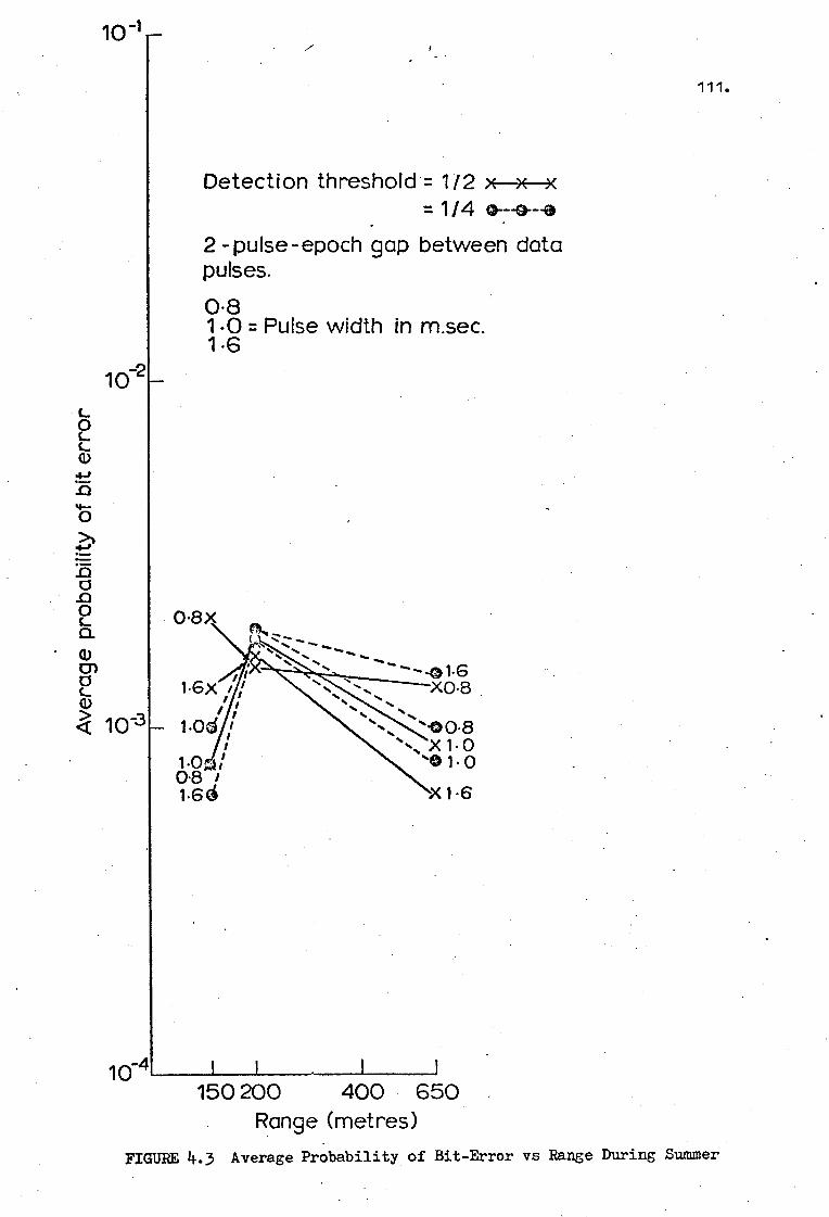
10 -1

Detection threshold = 1/2 x x x = 1/4 oT-e a•

2 - pulse - epoch gap between data pulses.

0.8 1.0 = Pulse width in m.sec. 1.6

I

102 L 0 L L

O

:Ei .0 O L a a) rn L a) > 1 0-3 itt

o-4 I

150 200 400 650 Range (metres)

FIGURE 4.3 Average Probability of Bit-Error vs Range During Summer

1.0

0.8x 1.6

`-x X1-0 X0.8

1.6

112.

Detection threshold = 1 / 2 x x -1/4

1- pulse- epoch gap between data pulses.

0.8 1.0 = Pulse width in m.sec. 1.6

10-2

O

.0

.0 O a

a a) > < 10

10 -4

ON % 8 %

0'8itt I r

. • . . . IN s I 'N. I _ ..N.------00.8, 1.0

------ .. 1 e• i ■ . 1.0 . %, 1.6

1.6

1 150 200 650

Range (metres) FIGURE 4.4 Average Probability of Bit-Error vs Range During Summer

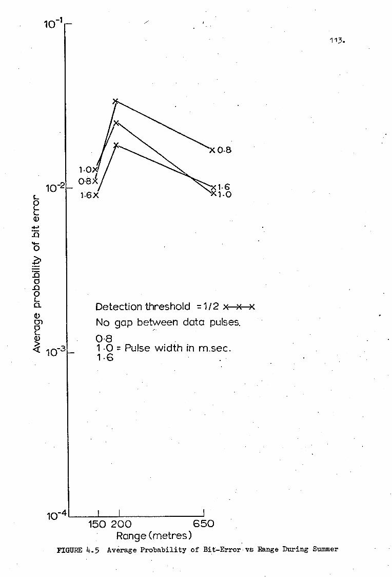
10-1 113.

102 L 0 L L

.0

0

4?) .0 0 .0 O L 0. cn

< 10-3

Detection threshold =1/2 x— --xNo gap between data pulses. 0.8 1-0 = Pulse width in m.sec. 1.6

10-4 150 200 650

Range (metres) FIGURE 4.5 Average Probability of Bit-Error vs Range During Summer

114.. Detection threshold =112 Range = 650 metres

x = 1.6 m. sec. pulse width o= 1.0 m. sec. pulse width A = 0.8 m. sec. pulse width

10-2 L 0 L L a) .0•

5

15

0 L CL

a) cn 0 L a) < 10-3

10-4 2 1 0

Gap between data pulses (pulse epochs) FIGURE 4.6 Average Probability of Bit-Error as a Function of Data-Rate

During Summer

10-1

115.

Detection threshold =1/2 x x x =1/4 o—o—o

2-pulse-epoch gap between data pulses

0.8 1 .0 = Pulse width in m.sec. 1.6

10-2

Aver

age

pro

babi

lity

of b

it e

rror

io-3

FIGURE 4.7 Average Probability of Bit-Error vs Range During Autumn

io-4 1 150 200 650

Range (metres)

10-1 116.

Detection threshold =1/2x—x—x =1/4 G.-9—ca

1-pulse-epoch gap between data pulses.

0.8 1.0 =Pulse width in m.sec. 1.6

"6

FIGURE 4.8 Average Probability of Bit-Error vs Range During Autumn

104

I 1 I

150 200 650 Range (metres)

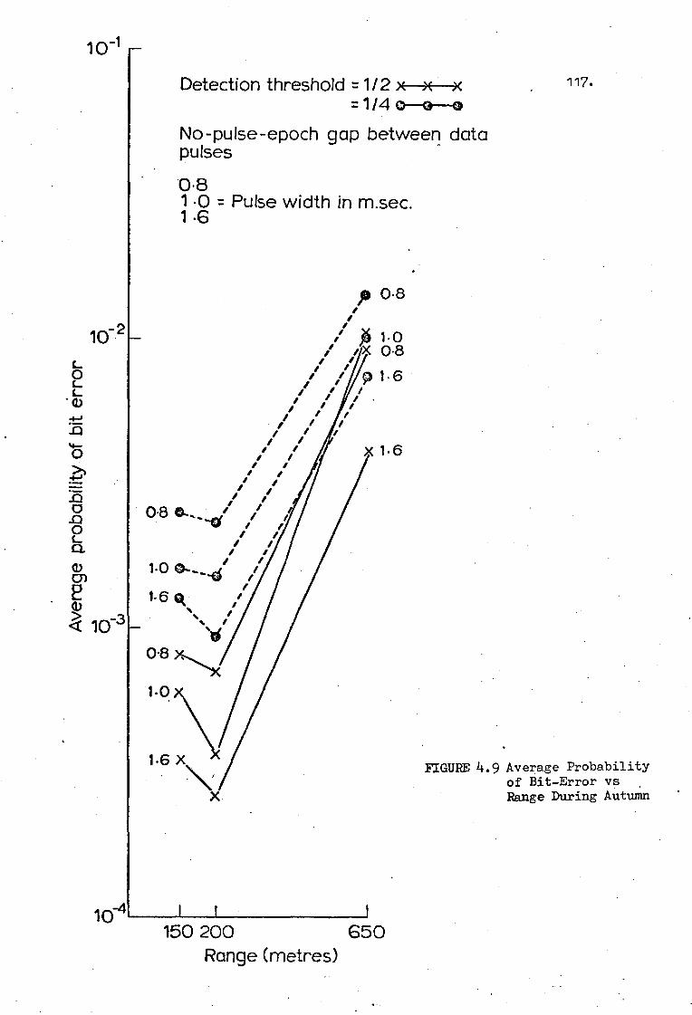
0.8 x

1.0

1.6 X

10-1 117. Detection threshold =1/2

=1/4 o—o---o

No-pulse-epoch gap between data pulses

0.8 1 -0 = Pulse width in m.sec. 1.6

p 0.8

10- 2 / i A 1.0 / , X 0.8 L . 0 . / ,/ / 9 1 . 6 L._ . / L. / / / / , . /

7,-1 . / -0 I

/ //I i /

45 , . . . x 1.6 .1.?,' / , . I

. , -VD / i

1 i • ..--z-- 1

0.8 e.. / / n .....01 / // 0 L / /

/ / 0. / 1

0(1) 1•0 0•••...,1 / ) /

1-6 et . 4tC

I 2 . I ..,. • /

10_3 • I •

FIGURE 4.9 Average Probability of Bit-Error vs . Range During Autumn

150 200 650 Range (metres)

10-1

118. Detection threshold = 1/2 Range =650 metres

x = 1.6 m.sec. pulse width o =1.0 m.sec. pulse width A = 0.8 m.sec.pulse width

L 10-2 O L L

FIGURE 4.10 Average Probability of Bit-Error as a Function of Data-Rate During Autumn

10-4 2 1

Gap between data pulses (pulse epochs)

1.0 0.8

1.6

102 L 0 L L a)

75

.0 cs 0

N 0 L as

1

10-1 119.

x 2-pulse-epoch gap between data pulses o 1 " II fl II

A 0 18 II If 11 Si IS

1. 0 m.sec. pulse width

FIGURE 4.11 Average Probability of Bit-Error During Autumn with an Absolute Fixed Threshold

150200 650 Range (metres)

10.

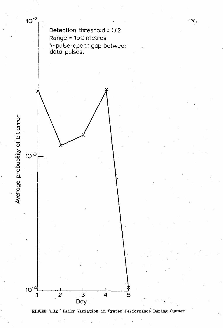
io-3

- 10 2 120. Av

e rag

e pr

o bab

ility

of

b it

err o

r

• Detection threshold = 1/ 2 Range = 150 metres 1-pulse-epoch gap between data pulses.

FIGURE 4.12 Daily Variation in System Performance During Summer

10-41 2 3

Day 4

10-1 121.-

Detection threshold =1/2 Range =150 metres

1- pulse -epoch gap between data pulses. x- r; 1.0 m. sec. pulse width

102 L O L L

.0

tax

15

.0 0

O L

cn 0 L • sz

10-3

x

J 2

Day FIGURE 4.13 Daily Variation in System Performance During Autumn

10 4

122.

performance during the summer period was found to be associated mainly

with the rapidly changing thermal conditions within the reservoir and

with the fact that a large mechanical pump was used during the summer

to stir the water in the reservoir. Because the thermal

characteristics of the reservoir could change considerably within the

space of twenty-four hours, marked changes in the refractive index of

the medium could result. This would lead to significant changes in

the fluctuations of the received signals and thus, a considerable

variability in system performance could result. To investigate this

aspect further, a study of the performance of the system was examined

during an arbitrarily chosen five-day period, and the results of the

examination are shown in FIGURE 4.12. From the figure, it can be seen

that the measured bit-error probability changed quite significantly

during the five-day period.

The material contained in FIGURES 4.3 to 4.5, and more particularly,

in FIGURE 4.6, provides information about the way in which the

probability of bit-error varies as a function of range and data-pulse

width. The figures show that if the gap between data-pulses is

increased from one pulse width to two pulse widths, there is virtually

no change in the probability of error, but if the gap is reduced to

zero, then the probability of bit-error is increased significantly.

, This increase in the error probability is due to intersymbol

interference in the form of multipath propagation. The geometry of the

reservoir and the absorbent nature of its bottom were such that the

multipath took the form of a single echo from the water surface with

the echo spreading into the immediately adjacent pulse epoch.

4.3 Interpretation and Analysis of the Autumn Results

The results contained in FIGURES 4.7 to 4.11 indicate that during

123.

the autumn period, the performance of the data transmission system

remained relatively constant, and in many respeCts, the performance is

easier to predict and understand than in the case of the summer results.

During the autumn, the thermal conditions within the reservoir changed

very little from day to day, and the transmission characteristics of

the medium were found to remain correspondingly constant. To investigate

the system performance further, as in the summer case, a study of the

performance of the system during an arbitrary five-day period was carried

out. The results are shown in FIGURE 4.13. The figure reveals that,

during the autumn period, the system performance changes very little

from day-to-day.

From FIGURES 4.7 to 4.9, it can be seen that in most cases, the bit-

error probability tends to increase with increasing range for all data

pulse widths and detection thresholds. This trend is to be expected

because of the fact that, for a constant transmitter power, the signal-

to-noise ratio decreases for increasing range.

The effect of intersymbol interference on the average bit-error

probability can be seen in FIGURES 4.7 to 4.9, and more particularly

in FIGURE 4.10. A comparison of FIGURES 4.6 and 4.10 shows that during

both the summer and autumn periods, there is a sharp increase in the

bit-error probability when the gap between adjacent data-pulses is

decreased from one pulse width to zero.

An examination of FIGURE 4.11 provides further insight into the

performance of the ASK data transmission system. The results shown in

the figure were obtained under the condition of a fixed absolute

threshold level for all test ranges. In the tests, the threshold

level was set at - of the received average signal amplitude at the

650-metre range and held constant at this value for all other ranges.

124.

From the figure, it can be seen that the average probability of bit-error

remains relatively constant for all ranges. Although the reasons for

this fact are not immediately obvious, a consideration of the probability

density functions of the background noise and the signal amplitude throw

some light on the matter. It will be shown ( see Section 4.5 ) that the

optimum detection threshold level varies from approximately 0.45 at 650

metres to about 0.15 at 150 metres, and that the PDFs of the received

signal amplitude vary in a manner illustrated in FIGURE 4.14. It has

been found, experimentally, that the errors due to false dismissals tend to

remain fairly constant for all test ranges. This is illustrated by areas A

and B in the example PDFs shown in FIGURE 4.14.

The effect of the receiver detection threshold on the average bit-

error probability can be observed from FIGURES 4.7 to 4.9. From the

figures, it can be seen that at the 150-metre range, a threshold of

produces a lower bit-error probability than does a threshold level of

but at the 650-metre range, the opposite tends to be true. It is not

clear, at this time, why this should be so. The difference in results

obtained with the two thresholds is quite small for each range and it

does not appear possible to draw any firm conclusions from the

measurements. Similar types of rather inconclusive results have been

obtained during the summer period, as illustrated in FIGURES 4.3 to 4.6.

The autumn results presented in FIGURES 4.7 to 4.11 show that,

irrespective of the range, the data-rate, and the detection threshold,

the probability of bit-error decreases slightly with increasing data-

pulse width. However, further tests have shown that if the data-pulse

width is increased beyond 1.6 msec to 2.0 msec, then there is no

further reduction in the bit-error probability. The slight improvement

resulting from the use of wide pulse widths can be explained in terms

pro

bab i

lity

PDF (noise)

PDF (long range) {111 AREA A

PEI AREA B

PDF (short range)

4 Optimum threshold at short range amplitude Optimum threshold at long. range

(absolute threshold used at all ranges - see FIGURE 4.11)

FIGURE 4.14 Illustration of the Variation of the Signal PDF with Range

126.

of the slight timing jitter and pulse amplitude fluctuations that were

observed during the tests. The operation of the sampling pulse in the

error-counting section of the receiver was governed by the bit-

synchroniser circuit. The synchroniser was capable of adjusting the

receiver clock in 50 lisec increments and this resulted in a timing

jitter in the sampling operation. Narrow pulse-width systems, in which

the decisions are taken by sampling the received data pulse and comparing

the sample amplitude with a threshold, are more sensitive to the

combination of timing jitter and amplitude fluctuations than are systems

using wider pulses. It will be observed from FIGURES 4.7 to 4.11 that

the improvement resulting from increasing the data-pulse width is only

slight, and the reduction in data-rate that results from increasing the

data-pulse width would be hard to justify in a practical data transmission

system.

4.4 A Comparison of Predicted and Measured Bit-Error Probabilities

It is useful to be able to predict, theoretically, the performance

of the underwater data transmission system in terms of the average bit-

error probability. In order to do so, a knowledge of both the noise

PDF and the signal-plus-noise PDF is required. In Chapter 3, two PDF

models of the sampled signal amplitude fluctuations were derived based

on wind directions which were approximately perpendicular and parallel

to the direction of transmission. Since these specific conditions will

occur relatively infrequently, it is important to know whether the PDF

models derived in Chapter 3 can be used in the more general situation

in which the wind direction is at any angle to the line of transmission.

In this section, the performance of the ASK system is examined in terms

of the predicted and measured average bit-error probabilities.

If the data transmission rate is sufficiently slow, then inter-

127.

symbol interference effects can be avoided. In the test system, which

is described in Chapter 2, a form of envelope detection was used in the

data receiver. The average probability of error in a binary communication

system in which envelope detection is used in the receiver can be written

in the form,

P(e) = Pfs(e) + Pfd(e)

=o n

(r)dr + P1

fs(r)dr (4.1)

T C)

where Pfa(e) and Pfd

(e) are the false alarm and false dismissal

probabilities respectively; P1 and Po are the a priori probabilities

of a binary 'one' and a binary 'zero' respectively; fn(r) is the PDF

of the demodulated noise; fs(r) is the PDF of the signal-plus-noise;

and T is the detection threshold level.

For envelope detection, the demodulated noise PDF will be a

Rayleigh distribution. In the underwater data transmission system used

in the tests, a 5% carrier was transmitted when a binary 'zero' was

sent. The resulting demodulated output of the receiver in this case

would not be Rayleigh distributed but Rician distributed ( Rice, 1954).

However, the amount of carrier present when a binary 'zero' is transmitted

is small and the resulting PDF can be approximated by a Rayleigh

distribution of the form,

fn(r) = exp

N2 [ 2N2 o

where No2 is the noise power.

X This is the case for true 'ON/OFF' ASK systems.

(4.2)

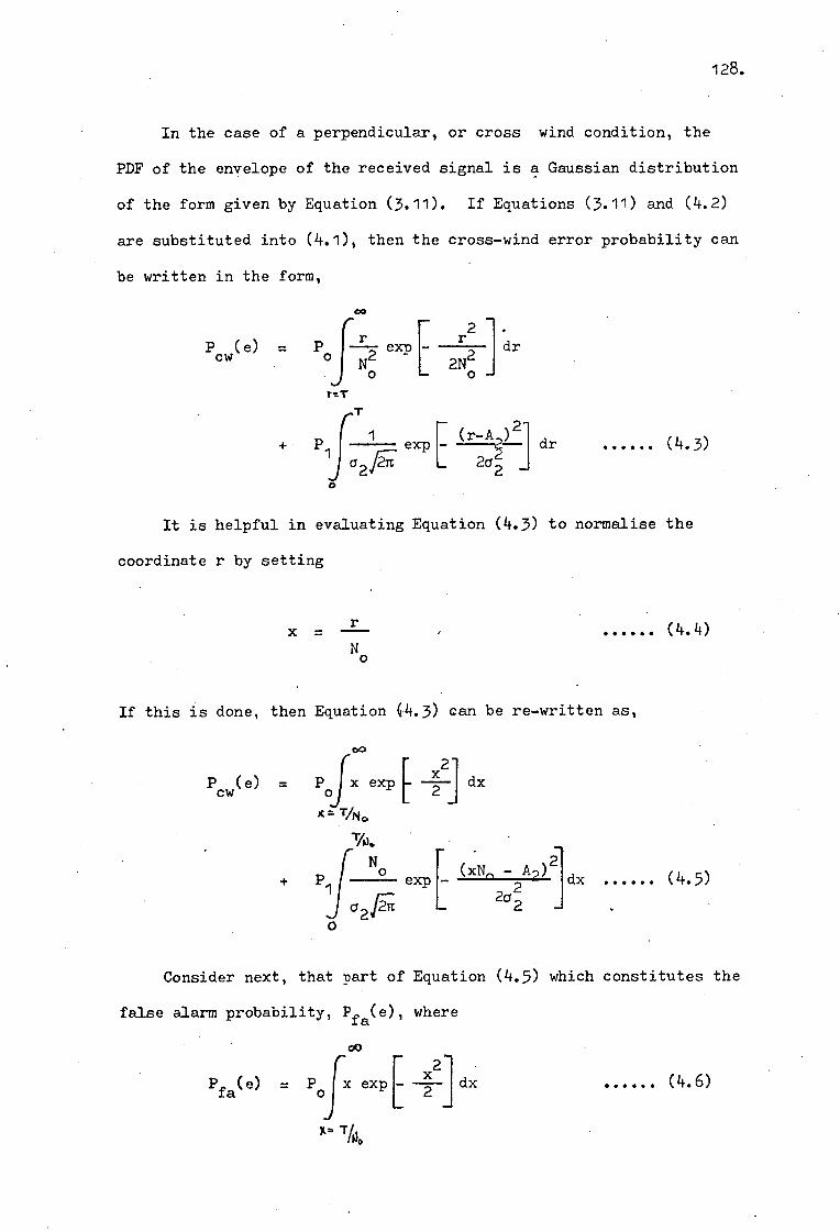
128.

In the case of a perpendicular, or cross wind condition, the

PDF of the envelope of the received signal is a Gaussian distribution

of the form given by Equation (3.11). If Equations (3.11) and (4.2)

are substituted into (4.1), then the cross-wind error probability can

be written in the form,

CO

2 I. P (e) = P -E- exp r dr cw o N2 2N:

0 T

2 plf1 xp [ (r -A ) 1 dr (4.3)

a2[--rt 20

0

It is helpful in evaluating Equation (4.3) to normalise the

coordinate r by setting

r X = ---

N

( 4 . 4 )

If this is done, then Equation (4.3) can be re-written as,

00 2

P (e) = cw Po fx exp [ 2 dx

exp[ (xN -A2).I dx No n (4.5)

2 202 F.,

Consider next, that part of Equation (4.5) which constitutes the

false alarm probability, Pfa(e), where

oo

ri

x2 Pfa(e) = Po x exp -2 1 . [ --- dx

x= 7 A4

(4.6)

Va.

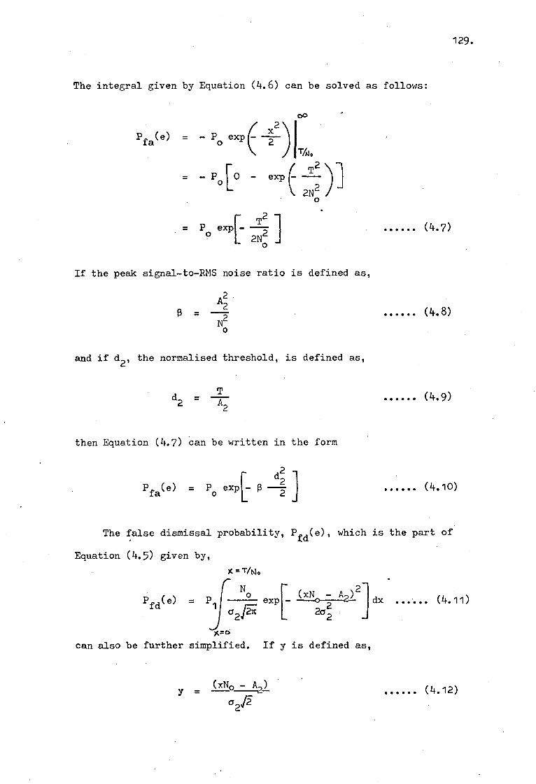
129.

The integral given by Equation (4.6) can be solved as follows:

00

2 Pfa(e) = - Po exp -a--) 2

T440 ,T,2

= Po [0 - exp )1

2N2

T2

= Po exp[ --7 2No

(4.7)

If the peak signal-to-RMS noise ratio is defined as,

2

0 A2

(4.8) N2 0

and if d2, the normalised threshold, is defined as,

d2 A2

(4.9)

then Equation (4.7) can be written in the form

pfa(e) = Po exp 0 dp

2

(4.10)

The false dismissal probability, ( ), which is the part of

Equation (4.5) given by, K=T/N0

(e) =

No exp (xNo A2)2

dx :1

(4.11)

2 [ 2a2 2

K=o can also be further simplified. If y is defined as,

(xN0 - A — ) y = — 2—

ada-

(4.12)

130.

then by substitution of (4.12) into (4.11), Pfd(e) becomes,

b LIAL Q,J

1 Pfd(e) = P1

exp(-y2) dy Ft

(4.13)

3' -A%

Equation (4.13) may be further simplified by the consideration of

the symmetry properties of a Gaussian distribution. If ARG is

defined to be,

, ARG = 1 expl-y (4.14)

then, T- AL cz tn.

Pfd(e) = P1 ARG dy (4.15)

-Az doh

The total area under a normalised Gaussian distribution is, therefore,

PIRG dy 1--AL 7,72.

+ JARG dy

-AL

+00

+ARG dy = 1 f

(4.16)

-r- AL tr z Arz

If the complementary error function is defined as, .

00

erfc(w) = 2 exp(-t2) dt (4.17)

131.

then Equation (4.16) can be expressed as,

4VIcsji

j'ARG = 1 - ierfc(T A;) ,12 ARG (4.18) ,

Moreover, if the value of -A2/62J2 is sufficiently large ( i.e.

a high signal-to-noise ratio ), then the last integral in Equation

(4.18) becomes very small or in other words,

Li= 761. Jr cron.

I ARG J -a,

(4.19)

By using the identity,

erfc(-x) = 2 - erfc(x) (4.20)

the false dismissal probability can be written in the form,

Pfd(e) = P1 [ierfc((A74q a 4e

On setting T = A2d2 and Vz a2/A2, it follows that

Pfd(e) = P1 [ierfc(111-(111

Vzjf

(4.21)

(4.22 )

Thus, the average probability of error in the perpendicular-wind case

can be given as,

a2 P cw(e) = + Pi 4erfc L:112.) (4.23)22

VznlC

(e) PPw

= Po exp 2 No

2 r2 dr ] 2N o

r a i If

and

(4.27)

V =

Ai a = -7-

CI

132.

In the case of a wind which is parallel to the direction of

transmission, the PDF of the envelope of the signal is a Rician

distribution as given by Equation (3.0. By substitution, the

parallel-wind bit-error probability, PPw

(e); is

00

r-T

+ P1 r ex 2 p

_Jr a

2 2 1 I _ 11±W IL dr 2 o 2 2a1 a

(4.24)

0

The false alarm probability, which is given by the first integral

in Equation (4.24), is of the form similar to Equation (4.10) and

can be expressed as,

Pfa(e) = Po exii- .14] (4.25)

where d/ = T/A l.

The false dismissal probability can be expressed in the form

of the Q-function (Marcum, 1950), where the Q-function is defined as,

oo

Qta,b1 = jry exp 2[ (a2+v2)"]

Io(av) dv

6

(4.26)

then the false dismissal probability, which is the second integral

in Equation (4.24), can be expressed in the form,

133.

Pfd(e) = P1 v exp (a2.01.2)

1 Io(av) dv (4.28)

0

Equation (4.28) is simply ( 1 - Qta,T a3) and hence,

Pfd(e) = P1 1 - Q ' TT,

If VI = a /A, and d1 = T/A1 , then

V ' Pfd(e) = P1 1 - Q ' 1 17 Vi I

(4.29)

(4.30)

Thus, the average probability of bit-error in the parallel-wind case

is given by,

d

PPw (e) = Po[exp(- d2 + P1 - 17

, 11 (4.31)

The perpendicular-wind and parallel-wind error probabilities

(Equations (4.23) and (4.31) are expressed in terms of the peak

signal-to-r.m.s. noise ratio, 0, the coefficients of variation, V1

and V2' and the normalised detection thresholds' d1 and d2.

By using

suitable values for these parameters, it is possible to compute

average bit-error probabilities for both the perpendicular-wind and

parallel-wind propagation conditions. Since T = dA, a particular

value of d represents the detection threshold normalised to the

average signal amplitude, A. In the results which follow, a value

of d1 = d2 = 0.5 was used in the computation of Equations (4.23)

and (4.31). This particular value of d was also the value of the

threshold level used at the reservoir during the experimental tests.

V=T cri

134.

The values for V1 and V

2 have been given previously in FIGURES

3.11 and 3.12 and in TABLES 3.1 and 3.2. The computation of Equations

(4.23) and (4.31) was based on values of Vz and V I which were

determined over a 25.0 second time interval. These 'long-term'

values were used, rather than the 2.5 second 'short-term' values,

because the longer term values are more representative when comparing

the measured average bit-error probabilities with the predicted

error probabilities. This is on account of the fact that the

measured error probabilities were determined over a period of

several minutes for each error test.

Values of the peak signal-to-RMS noise ratio, p, were measured at

the reservoir for all test ranges and these measured values are shown

in FIGURE 4.15. Also shown in this figure are computed values of S/N

ratios based on the measured value at the 150-metre range. The computed

values for the 200 and 650-metre ranges were then calculated from

a consideration of spherical divergence and losses due to absorption

( see Chapter 2 ). From FIGURE 4.15, it can be seen that the

measured values of 0 are in close agreement with the computed values.

By using the appropriate values of V1, V2

and p in Equations

(4.23) and (4.31), it is possible to compute error probabilities

for both the perpendicular-wind and parallel-wind cases respectively.

The computed bit-error probabilities, with Po = P1 = 0.5, and the

experimentally determined values are shown as a function of 0 in

FIGURE 4.16. The measured values shown in the figure were obtained

from tests carried out during both the summer and autumn periods.

From FIGURE 4.16, it can be observed that at S/N ratios above 17 dB, the

parallel and perpendicular-wind model predictions appear to be upper and

lower bounds to the measured bit-error probabilities, but that the

S/N is used as an abbreviation for peak signal-to-RMS noise

30

0 100 200 150 65o 800 Li 00

135.

/D Computed Values

X- -- - -X Experimentally Measured Values

RANGE (metres)

FIGURE 4.15 Measured and Computed Peak Signal-to- RMS Noise Ratios

Autumn Result

136.

10 2

10-3

10 4

Parallel-Wind Model Prediction

Summer Result • .

• • •

10 5

AVER

AGE

PR

OB

AB

ILIT

Y O

F B

IT-E

RRO

R

10 7

10-6

10-8

lo 9

Perpendicular-Wind Model Prediction

1012

1 1 1 1 I 1 i I

12 14 16 18 20 22 24 26 28

PEAK SIGNAL-TO-RMS NOISE RATIO (dB)

FIGURE 4.16 Computed and Measured Error Probabilities

30

137.

measured data lies closer to the upper bound than to the lower bound,

particularly at the high values of signal-to-noise ratio. There are

two main facts which may account for this trend.

Firstly, the derivation of the PDF models used in the computation

of the bounds was based on the assumption that there was no time delay

between the direct-path and surface-reflected-path signals. However,

at the 150-metre range, this assumption is of somewhat limited

validity because of the significant time delay between the two signal

paths. This time delay would affect the parameter, V. This parameter

was determined from the received signal PDFs which were obtained by

sampling the received data-pulses at the centre of each data-pulse.

If the two signals arriving from the direct-path and surface-reflected-

paths were not coincident in time, then the measured value of V would

not be totally representative of the actual value. It is thought that,

particularly at the 150-metre range, the measured values of V are

somewhat lower than the values which would be obtained if the two

signals were coincident.

A second factor which can explain the results shown in FIGURE 4.16

is the effect of the prevailing wind direction on the average bit-

error probabilities. Although the measured results were obtained

under a variety of wind directions, it was found that the majority

of the experimental tests were recorded under a prevailing parallel-

wind condition. Thus, the measured results would tend•to be 'biased'

towards the upper bound, as illustrated in FIGURE 4.16.

It can also be seen that at S/N ratios less than 17 dB, the measured re✓ults

are not bounded by the values computed from the perpendicular-wind

model prediction. A possible explanation for this is that at the

long ranges, which are associated with the lower values of signal-

to-noise ratio shown in FIGURE 4.16, multiple reflections may have

r ro2

(ro-Aa)2

exP[

exp 1

2 oz N"` 2 No 2N2

( 4. 33 )

138,

occurred and the Gaussian model may be of somewhat limited validity.

However the Rician model, as used in the parallel-wind case, would

still be applicable provided the relative phase fluctuations between

the various steady components of the reflected paths were small.

4.5 Optimum Fixed Detection Threshold Level

Further information about the way in which the signal PDF

changes with wind direction and range can Be obtained by an analysis

of the optimum fixed detection threshold level which minimises the

average probability of bit-error. It is possible to compute the

optimum fixed threshold from an analysis of both the noise PDF and

the signal-plus-noise PDF. If the a priori probabilities, Po and

P1' are equal, then by using the Bayes decision strategy, the

optimum fixed threshold can be found by determining the point at

which the value of the signal-plus-noise PDF is equal to the value

of the noise-only PDF. To be more explicit, the optimum threshold,

ro, can be found when ( see Schwartz, Bennett and Stein, 1966 ) 1

fs(ro) Po

fn(ro) - P

1

= 1 (4.32)

where f 8 (r 0) and fn(ro) are the signal-plus-noise and noise PDFs

respectively, and ro is the optimum fixed detection threshold level.

In the case of a wind which is perpendicular to the direction

of transmission, the minimum probability of error can be found by

setting Equation (4.2) equal to Equation (3.11); that is when,

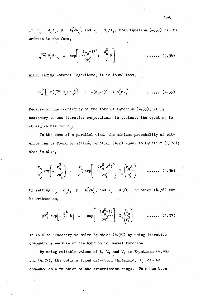
139.

If, ro = doA2, 0 = A2 /No2 , and Vz = a2 /Ay, then Equation (4.33) can be

written in the form,

1 (d -1)2 d2 o .„

Ft Vz Odo = exp - 2 + — p 2Va 2

After taking natural logarithms, it is found that,

(4.34)

2V2 [ ln(J VZ 0d0)] = -(d0-1)2 + do2 0V2

(4.35).

Because of the complexity of the form of Equation (4.35), it is

necessary to use iterative computations to evaluate the equation to

obtain values for do.

In the case of a parallel-wind, the minimum probability of bit-

error can be found by setting Equation (4.2) equal to Equation (3.7);

that is when,

- , ro

r02

r0 kr02 4-A2l! roAl

exp - exp No 2No2

0

2 1 2a2

0 (4.36)

On setting ro = d0A1 , 0 = 4/N(2), and VI = al /A l , Equation (4.36) can

be written as,

2 (do+1) pv2 exp[7 13] = exp[ 1 '(1 )

1.

2 do 2 0 2 2V1 VF

( 4.37)

It is also necessary to solve Equation (4.37) by using iterative

compuations because of the hyperbolic Bessel function.

By using suitable values of 3, Vz and VI in Equations (4.35)

and (4.37), the optimum fixed detection threshold, do, can be

computed as a function of the transmission range. This has been

140.

done and the results are shown in FIGURE 4.17. In the figure, the

computed threshold levels are shown for both the perpendicular and

parallel-wind cases.

From an analysis of FIGURE 4.17, it can be seen that for both the

perpendicular and parallel-wind cases, the optimum fixed detection

threshold level increases with increasing range. This phenomenon

can be explained in terms of the peak sigrial-to-RMS noise ratio

and the variances of the probability density functions of the signal-

plus-noise and noise amplitudes. At the shorter transmission ranges,

the peak si gnal-to-RMS noise ratio, was high, typically 25 to

30 dB. However, it was found that the variances of the signal-plus-

noise PDF was considerably larger than the variance of the noise-

only PDF, as illustrated in FIGURE 4.14. This implies that in order

to minimise the bit-error probability, it is necessary to reduce the

detection threshold setting to a value of less than one-half of the

average peak signal amplitude. However, at the long range (650

metres), the difference between the variances of the two PDFs was

found to be less than at the shorter ranges and hence, the optimum

threshold level is increased toward the relative value of 0.5 as

illustrated in FIGURE 4.17.

A further point that can be made from the information contained

in FIGURE 4.17 is that for all transmission ranges, the relative optimum

threshold level is lower in the parallel-wind case than in the

corresponding perpendicular-wind case. This can be explained in

terms of the coefficients of variation of the signal-plus-noise PDF

information that was presented in TABLES 3.1 and 3.2. In these

tables, it was shown that at all test ranges, the coefficient of

variation was larger in the parallel-wind case than in the

perpendicular-wind case. By taking account of the previous analysis

•

o. 6

Parallel-Wird 0.5

0 . 4 0

0

cz 0.3 E-1 z 0 E-1 U 4-1

0.2

W

0.1 0

Perpendicular-Wind

141.

0.0 1 1 4

100 150 200 . 400 650 8on 1000

RANGE (metres)

FIGURE 4.17 Computed Optimum Fixed Threshold Levels

142.

relating to the increasing detection threshold with increasing

range, then it is possible to explain the fact that the optimum

threshold will be lower in the parallel-wind case than in the

corresponding perpendicular-t4ind case.

The measured bit-error probabilities, in general, provide rather

inconclusive information about the effect of the detection threshold

level on the average bit-error probability. However, the data shown

in FIGURE 4.11 clearly supports the hypothesis that the optimum

threshold level increases with increasing range. The results shown

in FIGURE 4.11 were obtained under the condition of an absolute

fixed threshold level at all test ranges. The threshold was set at

one-half of the average peak signal amplitude at- the 650-metre range

and was then held constant at this level for subsequent tests carried

out at the 200 and 150-metre ranges. FIGURE 4.11 shows that the

average bit-error probability remains relatively constant for all the

test ranges when using the fixed absolute threshold level. Thus, as

the transmission range was decreased, and hence the peak signal-to-RMS

noise ratio was increased, the receiver detection threshold level,

in terms of the average peak signal amplitude, was decreased. More

explicitly, the actual threshold level changed from approximately

0.5 to 0.1 as the transmission range was decreased from 650 metres

down to 150 metres. Thus, if the actual fixed detection threshold

level used in this particular series of tests was approximately equal

to the optimum threshold level at each range, then it is possible

that the average bit-error probability would remain relatively

constant, as illustrated in FIGURE 4.11.

Although some of the experimental results have been in agreement

with the theory presented in this section, the majority of the results

143.

obtained with threshold settings of 0.5 and 0.25 of the average peak

signal amplitude at each test range do not provide any conclusive

evidence of the effect of the threshold level on the average bit-

error probability. It is clear that more work is required in the

investigation of the effect of the detection threshold level on the

bit-error probability and in the relationship between the measured

data and computed results.

144. CHAPTER FIVE

BASEBAND PULSE RESPONSE

Introduction

The baseband pulse response of a communication system is a parameter

that is highly important in system design. A detailed knowledge of the

pulse response, and the way it varies as a function of time, are

essential if the effects of pulse dispersion are to be understood and

neutralised. In this chapter, the baseband pulse response of the ASK

underwater data transmission system is considered and the results of a

preliminary practical investigation into some of the properties of the

response are presented.

5.1 Practical Derivation of the Baseband Pulse Res onse

There are two main methods which can be used to investigate the

properties of the communication channel. The first method, which is

well-established, involves the determination of the impulse response of

the channel. From an analysis of the impulse response, it is possible

to determine both the time and the frequency response of the channel.

Also, additional information about multipath interference and pulse

dispersion can be obtained.

Although the impulse response is perhaps the most convenient

method of expressing the properties of a channel, there are several

difficulties associated with its use. In practice, it is not possible

to generate ideal impulse signals and it is necessary, therefore, to

use finite-width pulses. As finite-width pulses have to be used, it is

necessary to apply deconvolution methods in order to obtain the impulse

response. The channel impulse response can be deconvolved from the

received signal in two ways,both of which can be implemented with the

aid of a digital computer. The first method involves the division, in

145.

the frequency, of the received signal spectrum by a replica of the

transmitted signal spectrum. Although this can be accomplished using

fast Fourier transform (FFT) programmes, the method requires exact

phase synchronisation between the transmitted and received signals.

If, for example, both the transmitted signal and received signal are

recorded on magnetic tape, then the phase information required in the

computation of the desired impulse response can be lost. This can be

explained as follows.

A signal, x(t), is transmitted through a linear network (or

channel), which has an associated impulse response, h(t). The

received signal, y(t), will therefore be the convolution of x(t) and

h(t), or,

y(t) = hwoc(t)

(5.1)

where eg■ denotes convolution.

If, however, x(t) and y(t) are recorded separately on magnetic tape

and then played into a digital computer through an analogue-to-

digital converter, then although y(t) is still the convolution of

x(t) and h(t), the recording of x(t) will be time-shifted when

compared to y(t), unless x(t) is exactly synchronised to y(t). Thus,

x(t) becomes x(t+T), where T is the time shift due to the absence of

synchronisation. If X(w), H(w), and Y(w) are the Fourier transforms

of x(t), h(t) and y(t), respectively, then the desired frequency

response of the channel can be given by H(w), where H(w) is

H(w) = Y(w)/X(w) (5.2)

If x(t) becomes x(t+T), then X(w) will be X(w)e-- , and therefore

the new frequency response of the channel is,

11+6.

Hqw) = H(w)e-jwT

(5.3)

It can be seen from Equation (5.3) that although the magnitude

frequency spectrum, 'HMI , is unchanged, or

111(co)I (5.4)

the phase spectrum has been altered by an amount equal to -wT. In

order to compute h(t) from H(w), both the phase and amplitude spectra

information are required. However, if the phase information of H(w)

is incorrect, as illustrated in Equation (5.3), then the desired, or

true response, h(t), cannot be computed.

A second method of deconvolving the channel impulse response from

the received signal is the use of complex cepstrum analysis ( Gold and

Rader, 1969 ). This method does not require phase synchronisation

between the transmitted and received signals and it is therefore

advantageous when compared with the previously mentioned method of

analysis. However, the cepstrum method is somewhat complex and

involves the use of a considerable amount of computer time.

In addition to the two main methods of analysing the channel

response, there is another method which can be used. This method

involves the use of the pulse response to determine information about

some of the properties of the channel. As in the case of impulse

response testing, an analysis of the pulse response can provide

information about multipath interference and pulse dispersion. The

pulse response method is very simple and requires little computer

time or programming. However, is does suffer from the disadvantage

that the overall time and frequency response of the channel cannot

be determined as easily.

The preliminary practical investigation into the pulse response of

147.

the ASK underwater system that is presented in this chapter is based on

the measurements of the pulse response of the system. In the

investigation, narrow-width raised-cosine pulses were transmitted and

the received pulse wave-forms were recorded and analysed. The results

obtained provide some fairly simple information relating to effects

such as multipath and pulse dispersion. It should be emphasised,

however, that the results are only provisional and that a much more

extensive investigation and analysis is required in order to take in a

wider range of operational and climatic conditions. It is necessary

that this should be done if general, wide-ranging, conclusions are to

be drawn.

5.2 Presentation of Experimental Results

The results in this section are presented on the basis of

measurements taken when the prevailing wind direction was approximately

parallel and approximately perpendicular to the direction of transmission.

Because of the effect that the prevailing wind direction has on other

factors such as the PDF and the amplitude frequency spectrum of the

signal, it was hoped that the analysis of the pulse response on a

similar basis would result in a deeper understanding of the behaviour

of the channel.

The tests were carried out at the reservoir over a period of

several months in order that measurements could be made under a variety

of climatic conditions. A sequence of 0.8 msec duration raised-cosine

pulses was transmitted at each range tested. The pulses were transmitted

with a repetition rate of one pulse every 6.4 msec and throughout the

test period, the transmitter power was held fixed at 50 milli-Watts

peak. When transmitting data pulses at a rate of 156 pulses per second,

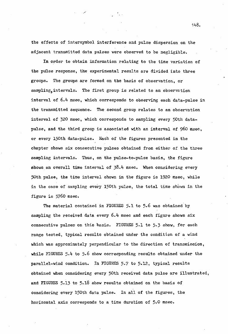
148.

the effects of intersymbol interference and pulse dispersion on the

adjacent transmitted data pulses were observed to be negligible.

In order to obtain information relating to the time variation of

the pulse response, the experimental results are divided into three

groups. The groups are formed on the basis of observation, or

samplinglintervals. The first group is related to an observation

interval of 6.4 msec, which corresponds to observing each data-pulse in

the transmitted sequence. The second group relates to an observation

interval of 320 msec, which corresponds to sampling every 50th data-

pulse, and the third group is associated with an interval of 960 msec,

or every 150th data-pulse. Each of the figures presented in the

chapter shows six consecutive pulses obtained from either of the three

sampling intervals. Thus, on the pulse-to-pulse basis, the figure

shows an overall time interval of 38.4 msec. When considering every

50th pulse, the time interval shown in the figure is 1920 msec, while

in the case of sampling every 150th pulse, the total time shOwn in the

figure is 5760 msec.

The material contained in FIGURES 5.1 to 5.6 was obtained by

sampling the received data every 6.4 msec and each figure shows six

consecutive pulses on this basis. FIGURES 5.1 to 5.3 show, for each

range tested, typical results obtained under the condition of a wind

which was approximately perpendicular to the direction of transmission,

while FIGURES 5.4 to 5.6 show corresponding results obtained under the

parallel-wind condition. In FIGURES 5.7 to 5.12, typical results

obtained when considering every 50th received data pulse are illustrated,

and FIGURES 5.13 to 5.18 show results obtained on the basis of

considering every 150th data pulse. In all of the figures, the

horizontal axis corresponds to a time duration of 5.0 msec.

149.

FIGURE 5.1 Perpendicular-Wind Pulse Response at 150 metres ( every consecutive pulse)

t ' 0 1 ' 2 3 4 5

TIME (msec)

150.

FIGURE 5.2 Perpendicular, Wind Pulse Response at 200 metres ( every consecutive pulse)

_ 0 1 2 3 4

TIME (msec)

151.

FIGURE 5..3 Perpendicular-Wind Pulse Response at 650 metres ( every consecutive pulse )

1 0 1 2 3 4 5

TIME (msec)

152.

FIGURE 5.4 Parallel-Wind Pulse Response at 150 metres ( every consecutive pulse )

0 1 2

5 TIME (cosec)

153.

FIGURE 5.5 Parallel-Wind Pulse Response at 200 metres ( every consecutive pulse )

t t

0 1 2 3 4 5 TIME (msec)

154.

FIGURE 5.6 Parallel-Wind Pulse Response. at 650 metres ( every consecutive pulse )

I L

0 1 2 3 4 5

TIME (cosec)

155.

FIGURE 5.7 Perpendicular-Wind Pulse Response at 150 metres ( every 50th pulse )

0 1 2 3 4 5 TIME (msec)

156.


1 I I * i 1 0 1 2 3 4

TIME (msec)

.157.

I t t t 1

0 1 2 3 If 5

FIGURE 5.9 Perpendicular-Wind PulSe Response at 650 metres ( every 50th pulse )

TIME (msec)

158.

I

FIGURE 5.10 Parallel-Wind Pulse Response at 150 metres ( every 50th pulse )

0 1 2 3 4 5

TIME (msec)

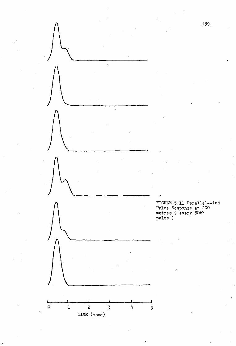
159.

4 0 1 2 3 TIME (msec)

5


160.


J

0 1 2 3

TIME (cosec)

5

161.


I t t I i 1 0 1 2 3 1+ 5

TIME (msec)

162.


I I I I I I. 0 1 2 3 4 5

TIME (msec)

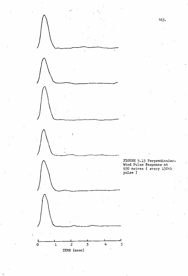
163.


F ( 1 I i

0 1 2 3 4 5 TIME (msec)

164.


0 1 2 3 4 5

TIME (msec)

165.


1 t t I t I 0 1 2 3 4 5

TIME (msec)

166.


i 1 1 I t t

0 1 2 3 4 5 TIME (cosec)

167.

A general observation which can be made from an analysis of the

results shown in FIGURES 5.1 to 5.6 is that, in each figure, the shape

and amplitude of the received data-pulses remain quite constant on a

pulse-to-pulse basis. Thus, as shown in each of the figures, the pulse

response appears to remain relatively constant, over a time interval

of 38.4 msec, for a particular range and prevailing wind direction.

An indication of the effect of the wind direction on the pulse

response can be seen from a comparison of FIGURES 5.1 and 5.2 with

FIGURES 5.4 and 5.5. In the case of a wind parallel to the direction

of transmission, as illustrated by the pulse responses in FIGURES 5.4

and 5.5, the multipath interference is such that the data-pulse width

is increased considerably. However, in the perpendicular-wind case,

as shown in FIGURES 5.1 and 5.2, the effect of the multipath

interference is much reduced and the pulse dispersion of the channel

does not appear to be as great as in the parallel-wind case. In general,

the responses shown in FIGURES 5.1 to 5.6 indicate that multipath and

pulse dispersion effects do not exist much beyond about 1.5 msec in the

case of either wind direction. It should be noted, however, that there

are some slight indications of pulse dispersion and multipath beyond

1.5 sec. This can be seen from a consideration of the responses shown

in FIGURES 5.3 and 5.6. These results, which were obtained at a range

of 650 metres, illustrate that some 'ripple' exists in the responses

beyond 1.5 msec. It is thought that multipath resulting in echo effects

could be a cause of this ripple.

Typical pulses responses obtained when considering every 50th

data-pulse are shown in FIGURES 5.7 to 5.12. From the figures, it can

be seen that, on a trace-to-trace basis, significant changes occur in

both the general shape of the received pulse and the pulse amplitude.

168.

In particular, this effect appears to be most pronounced when the wind

is parallel to the direction of transmission. This is illustrated in

FIGURES 5.10 to 5.12. In each figure, it can be seen that significant

changes in both the shape and amplitude of the data-pulses occur within

the time interlal of 1920 msec shown in the figure.

Further evidence of the nature of the multipath interference can

be obtained by considering the responses shown in FIGURE 5.11. It can

seen from the figure that the multipath signal appears first to increase

and then to decrease in the space of three or four traces. The time of

this variation ranges from approximately 700 to 1000 tasec. These values

approximately correspond to the time of the first, zero-crossing of the

autocorrelation functions presented in Chapter 3.

In FIGURES 5.13 to 5.18, which are results obtained by considering

every 150th data-pulse, it can be seen that, just as in the case when

every 50th pulse was considered, there are considerable changes in the

shape and amplitude of the data pulses and further that, in each figure,

this variation occurs on a trace-to-trace basis. The extent of the pulse

amplitude fluctuations is illustrated particularly in FIGURES 5.16 to

5.18. The responses shown in these figures were obtained under the

parallel-wind propagation condition. A comparison of FIGURES 5.16 to

5.18 with FIGURES 5.13 to 5.15 shows that the amplitude fluctuations

are larger in the parallel-wind case than in the corresponding case of

a perpendicular-wind

5.3 Summary of Results

It is important to note that the pulse responses presented in this

chapter are the result of only a preliminary investigation of aspects

relating to the pulse response of the channel. Although the results

are only provisional, they appear to be sufficiently uniform for some

169.

general indicative conclusions to be drawn.

One of the most significant observations which can be made is that

beyond approximately 1.5 msec, there is little multipath interference

or pulse dispersion. This would indicate that if data was transmitted

at a rate less than about 600 bits/second, then there would few false

alarm errors due to multipath effects. However, if the data-rate was

in excess of 600 bits/second, then errors due to false alarms arisng

from multipath interference would be introduced. This, in fact, has

been observed and is shown in FIGURES 4.6 and 4.10.

The material presented in FIGURES 5.7 to 5.12 provides an indication

of the 'fading-rate' of the multipath interference. From a consideration

of the figures, it can be calculated that fading-rates of the order of

1 Hz to 2 Hz occur and that these values are in agreement with results

relating to signal amplitude fluctuations presented in Chapter 3. This

type of information about the fading-rate of the channel is a highly

important parameter in the design and implementation of adaptive or

automatic equalisers. However, more work is required in the investigation

of the pulse response of the system in order to effectively implement

such methods of improving system performance Also, the effects of

increased range, and the associated increased multipath, need to be

investigated further.

170.

CHAPTER SIX

SUMMARY AND CONCLUSIONS

Introduction

In this chapter, the work presented in the thesis is summarised

and the conclusions which can be drawn from the results are described

in detail. Also, some suggestions are made relating to further research.

6.1 General Summary

Although the interest in underwater data communication has

increased considerably in recent years, there are many aspects relating

in particular to underwater data transmission that have not yet been

fully investigated. The aim of the work reported on in this thesis was

to investigate some of these aspects and to providb information about

them. It was intended mainly that certain important quantitative

results relating to the performance of a particular data transmission

system be obtained, and that the results be interpreted in terms of

physical and climatic conditions.

An ASK data transmission system was designed and tests using the

system were carried out in a large inland reservoir. The system is

described in Chapter 2, and an outline of the experimental procedures

adopted is also presented in the chapter. A presentation and analysis

of results relating to signal amplitude fluctuations is given in

Chapter 3 and, in Chapter 4, the performance of the ASK system is

studied in terms of the measured bit-error probabilities. In Chapter

5, a preliminary practical investigation into the pulse response of

the ASK system is presented and the results are discussed.

6.2 Summary of Results

In Chapter 3, the results of tests relating to the amplitude

171.

fluctuations of data pulses, transmitted over ranges of 150, 200 and

650 metres, are presented. Four parameters of the signal fluctuations

were computed. These were: the frequency spectrum of the envelope of

the signal, the autocorrelation function of the signal envelope, the

probability density function of the sampled signal, and the coefficient

of variation (or RMS amplitude fluctuationYof the received pulses.

An analysis of the computed amplitude frequency spectra and the

autocorrelation functions of the signal envelope has indicated that the

amplitude fluctuations of the received signal are dependent mainly on

the signal arriving from the surface-reflected transmission path. A

further study of these experimental results has revealed that the

signal fluctuations caused by the moving surface of the water are

affected by the direction of the prevailing wind, and it has been

found that when the prevailing wind direction is approximately parallel

to the transmission path, the effect of the surface-reflected signal on

the received signal is strongest. This fact was deduced from an

analysis of the amplitude frequency spectra. The results obtained

also indicate the effect of the surface-reflected path signal for a

wind perpendicular to the transmission path. However, under both

experimental wind conditions, the spectrum of the envelope of the

received data-pulses has been found to be similar to the amplitude

spectrum computed from a consideration of the wave-spectra theory of

Neumann and Pierson (1966), and the analysis of the signal autocorrelation

functions provides further evidence of this effect.

The probability density functions (PDFs) of the received data

pulses were computed from recorded data taken under a variety of

propagation and climatic conditions. It has been shown that if the

experimental data is divided according to the prevailing wind direction

172.

(as in the case of the autocorrelation functions and the amplitude

frequency spectra), then it is possible to compare the observed PDFs

with well-known distributions. In the case of a wind parallel to the

direction of transmission, the measured PDF has been shown to resemble

a Gaussian distribution, while in the perpendicular-wind case, the

experimentally determined PDF appears to tend towards a Rician

distribution.

A statistical analysis was carried out on the measured PDFs and

one of the statistics, the coefficient of variation, was studied in

detail in Chapter 3. Two main causes of signal amplitude fluctuations

were identified and separated from an analysis of experimental data

recorded under parallel-wind and perpendicular-wind propagation

conditions. It has been found that for a parallel-wind, the signal

amplitude fluctuations are caused by both the effects of the surface-

reflected path signal and the thermal inhomogeneities in the medium.

However, with a perpendicular-wind, the main cause of signal fluctuation

has been shown to be due to the thermal inhomogeneities within the

medium. It has also been shown that for a wind which was approximately

perpendicular to the transmission path, the fluctuations due to thermal

inhomogeneities agree closely with those predicted using the theory of

fluctuations developed by Chernov (1967). The fluctuations of the

signal caused by the effect of moving waves on the water surface have

been shown to decrease with increasing range, while the fluctuations

due to thermal inhomogeneities have been shown to increase with

increasing range.

An investigation relating to the PDFs of the direct-path and

surface-reflected path signals was also presented in Chapter 3. It is

seen that, under the conditions of a prevailing parallel-wind, the PDF

173.

of the surface-reflected path signal resembles a Rician distribution,

and that with a prevailing perpendicular-wind, the PDF of the signal

reflected from the surface resembles a Rayleigh distribution. An

explanation of these observations is given in terms of conventional

scattering theory. The PDF of the direct-path signal under both the

parallel and perpendicular-wind conditions has been found to approximate

to a Gaussian distribution. This is expected (see Whitmarsh et al, 1957)

in view of the ranges and the transmission frequency used in the tests.

Using the experimentally measured PDFs of the surface-reflected

and direct-path signal envelopes as a guide, two mathematical models of

the received signal envelope PDF have been developed. It is shown that

in the case of a wind parallel to the direction of transmission, the PDF

of the received signal envelope can be approximated by a Rician

distribution, while in the case of a perpendicular-wind, the resulting

envelope PDF of the signal approximates to a Gaussian probability

distribution. Experimentally measured PDFs have been found to be in

close agreement with the mathematical models.

The performance of the ASK data transmission system, in terms of

measured bit-error probabilities, was described and analysed in Chapter

4. The results were obtained over a period of several months and it

has been found that they could be interpreted more easily if they were

divided into two groups, namely those obtained during the period from

June to September (summer) and those obtained during the period from

October to November (autumn). The reason for dividing the groups in

this way was associated with the manner in which the temperature-depth

profile of the reservoir changed during the test period. It was found

that during the summer period, the temperature-depth profile could

change considerably over an interval of a lew days, while during the

174.

autumn period, very small changes in the temperature-depth profile were

observed during a similar interval.

The results of the bit-error probability tests indicate that, in

general, it is possible, when using only 50 milli-Watts peak transmitter

power, to transmit digital data over ranges up to 650 metres using a

carrier frequency of 150 kHz, and to do so with an average error

probability of 1 in 103, and that this can be done when transmitting

data at rates up to 625 bits/second. The results also indicate that if

data is sent at a rate of 1250 bits/second over the same ranges, then

this can be done, but that the average error probability is increased

to 1 in 10'?. An analysis of the results presented in Chapter .4 has

shown that errors in detection arise from two main sources -

intersymbol interference and signal amplitude fluctuations. When the

digital data is transmitted at rates below about 625 bits/second the

detection errors are due mainly to the effect of signal amplitude

fluctuations. These fluctuations can arise from both pulse dispersion

due to multipath interference, and thermal inhomogeneities in the

medium. However, if the data-rate is increased above 625 bits/second,

then additional detection errors occur and it is almost certain that

they are due to intersymbol interference resulting from the presence of

multipath.

The performance of the ASK data transmission system has been

found to be very dependent on the time of year during which the tests

were carried out. During the summer period (June to September), the

performance of the system, in terms of the measured bit-error

probabilities, was found to be extremely variable, and that the

variation could be significant from day-to-day. During the autumn

period (October to November), the system performance was found to be

175.

much less variable. It seems very likely that the variable nature of C ••

the system performance during the summer was related directly to the

significant variations in the. temperature-depth profile that occurred

from day-to-day.

The two PDF models developed in Chapter 3 were used in the

computation of the average error probability of the data transmission

system. Two computations, based on the PDF models derived for the

parallel and perpendicular-wind conditions, have been made for each test

range. It has been shown, in Chapter 4, that the computed error probabilities

based on the parallel-wind and perpendicular-wind PDF models appear to

form approximate upper and lower bounds to the experimentally measured

error probabilities. In particular, it is shown that for S/N ratios

greater than 17 dB, the measured results actually lie within the computed

bounds.

From an analysis and consideration of the results of tests

relating to the performance of the system in terms of the measured

bit-error probabilities, it is possible to draw some conclusions. It

has been shown that if the data-rate is less than approximately 625

bits/second, then communication can be carried out over ranges up to

650 metres, and that this can be done with an average bit-error

probability of 1 in 103. However, if data is transmitted at rates in

excess of 625 bits/second and a similar error-rate of 1 in 103 is to be

maintained, then it will be necessary to take steps to reduce the

effects of intersymbol interference and signal amplitude fluctuations.

It is suggested that techniques such as adaptive equalisation could be

used to achieve this objective.

The pulse response of the ASK system was considered in Chapter 5.

Although the investigation reported on in the chapter is only

176.

preliminary, several trends can be observed, and it is possible to draw

some indicative conclusions from the results of the investigation. It

is seen that the direction ofthe prevailing wind affects the amplitude

and shape of the pulse response. It appears that under the conditions

of a parallel-wind, multipath interference causes a considerable time-

spreading of the data pulses, but that under the conditions of a

perpendicular-wind, this effect is much reduced.

When considering the pulse response of the system in terms of a

pulse-to-pulse basis, it is seen that the response varies little during

the 38.4 msec analysis interval. However, if the response is

considered on the basis of.sampling every 50th data pulse, it is

observed that both the shape and the amplitude of the pulse response

change significantly over a 320 msec period. This is further

illustrated in the case when every 150th data pulse is sampled.

The analysis of the pulse response indicates that the multipath

interference changes from a maximum effect to a minimum effect in

approximately 700 to 1000 msecs. These particular time values compare

favourably with the values of the second zero-crossing of the signal

envelope autocorrelation functions which are presented in Chapter 3.

A conclusion which can be drawn from the experimental investigation

presented in Chapter 5 is that if techniques such as adaptive .

equalisation are to be implemented in order to improve system

performance, then the parameters of the equalisers will need to be

readjusted at rates of approximately two to ten times per second. The

equaliser will also be required to have a sufficient number of delay

taps in order to reduce the effects of pulse dispersion over intervals

of up to 1.5 msecs.

177.

6.3 Suggestions for Further Research

Although the work reported on in this thesis has provided some

valuable new information relating to several aspects of underwater

acoustic data transmission, much remains to be done. In this concluding

section of the thesis, several additional areas of investigation are

suggested and discussed briefly.

The tests relating to the average bit-error probability performance

of the ASK system have shown that, under the short-range shallow-water

conditions of the inland reservoir, it is possible to carry out

communication at a rate of approximately 625 bits/second over ranges up

to 650 metres, and to do so with an average bit-error probability that

is consistently of the order of 1 in 103. However, the investigation

has also indicated that if higher data-rates are to be achieved with a

similar bit-error probability, then it will be necessary to implement

techniques which are capable of reducing the effects of pulse dispersion

and intersymbol interference. One possible method of achieving this is

to implement adaptive equalisers into the system. A study of adaptive

equalisation techniques when applied specifically to the underwater

environment would therefore be very useful. The experimental

investigation of the pulse response of the channel has provided some

valuable information, which is useful in the design of equalisers,

relating to the characteristics of the multipath and pulse dispersion.

However, this information is only provisional and therefore, a more

detailed study of the pulse response of the channel is required.

The experimental investigation presented in the thesis has been

based on measurements made on an ASK data transmission system. It has

been shown that, when using ASK techniques, it is possible to obtain

information about the medium and its effect on system performance in

178.

a simple manner. It would be useful to assess the performance of under-

water data transmission systems, under similar propagation conditions,

but with other types of modulation methods. An interesting area of

research is the comparison of system performance when using ASK, PSK,

DPSK and FSK techniques. Other further areas of investigation are

carrier extraction methods in PSK systems when operating in a dispersive

medium, such as the underwater environment, and also the comparison of

various demodulation schemes in terms of the performance of the under-

water data transmission system.

The quantitative results relating to the study of signal amplitude

fluctuations, presented in Chapter 3, have been shown to be in agreement

with several relevent threories. Since the experimental investigation

has been carried out using one carrier frequency of 150 kHz, it would

be interesting to investigate the validity of the theories when using

different carrier frequencies in the ASK system. Further aspects of

this type of investigation are the study of the signal fluctuations

when using other modulation methods, and the study of phase fluctuations

with particular emphasis in PSK, DPSK and FSK systems. Similar types of

studies could be carried out, using several modulation methods, on the

signal probability density functions.

Perhaps a most interesting and challenging extension of the work

presented in this thesis is to apply the measurements and tests in

longer-range and deeper-water environments. The tests described in the

thesis can be carried out over a variety of transmission ranges and

propagation conditions and aspects such as signal amplitude fluctuations

and bit-error probabilities can be studied in detail in order that a

wider knowledge of underwater data transmission can be obtained.

179. REFERENCES

ABOTTEEN,R.A., SBEHADEH,N.M., and VANELLI,J.C. : ' Error Probability

of a Binary NRZ Signal Over a Parallel Channel ', IEEE Trans.

Sonics and Ultrasonics, Vol. SU-21, p300, 1974

ANDREWS,R.S., CONSTANTINIDES,A.G., and TURNER,L.F. : ' Use of Sample-

and-Hold Delay Circuits for Synthesising Raised-Cosine Filters ',

Proc. IEE, Vol. 121, p169, 1974

ANDREWS,R.S. and TURNER,L.F. : ' An Investigation of the Amplitude

Fluctuations of High-Frequency Short-Duration Sound Pulses Propagated

Under Short-Range Shallow-Water Conditions ', J. Acoust. Soc. Am.,

Vol. 58, No. 2, p331, 1975

ANDREWS,R.S. and TURNER,L.F. : On the Perform. ce of Underwater Data

Transmission Systems Using Amplitude-Shift-Keying Techniques ',

IEEE Trans. Sonics and Ultrasonics, Vol. SU-23, p64, 1976

BECHMANN,P. and SPIZZICHINO,A. : "The Scattering of Electromagnetic

Waves from Rough Surfaces", Pergamon Press, London, 1963

BENDAT,J.S. : " Principles and Applications of Random Noise Theory ",

J.Wiley and Sons, New York, 1958

BENNETT,W.R. and DAVEY,J.R. : "Data Transmission", McGraw-Hill Book

Company, New York, 1965

BERGMANN,P.G. : ' Propagation of Radiation in a Medium with Random

Inhomogeneities ', Physical Review, Vol. 70, p486 1946

BERKTAY,H.O., GAZEY,B.K., and TEER,C.A. : ' Underwater Communication -

Past, Present and nature ', J. Sound and Vib., Vol. 7, p62, 1968

CAMPANELIA,S.J. and FAVRET,A.G. : ' Time Autocorrelation of Sonic Pulses

Propagated in a Random Medium ', J. Acoust. Soc. Am., Vol. 46,

p1234, 1969

180.

CHERNOV,L.A. : "Wave Propagation in a Random Medium", Dover Publications,

New York, 1967

GODDARD,G.C. : 'An Underwater Acoustic Telemeter for Use in a Multipath

Channel', Ph.D. Thesis, University of Birmingham, 1970

GOLD,B. and RADER,C.M. : "Digital Processing of Signals", McGraw-Hill

Book Company, New York, 1969

HEARN,P.J. : 'Underwater Acoustic Telemetry', IEEE Trans. Comm. Tech.,

Vol. COM-14, p839, 1966

KINSLER,L.?. and FREY,H.R. : "Fundamentals of Acoustics", J. Wiley &

Sons, London, 1962

LIEBERMAN,L. : 'The Effects of Temperature Inhomogeneities in the Ocean

on the Propagation of Sound', J. Acoust. Soc. Am., Vol. 23, p563,

1951

MACKENZIE,K.V. : 'Long-Range Shallow-Water Signal Level Fluctuations

and Frequency Spreading', J. Acoust. Soc. Am., Vol. 34, p.61, 1962

MARCUM,J.I. : 'Table of Q-Functions', Rand Research Memo, RM339, 1950

MARSH,D.E. and ROWLANDS,R.O. : 'Upper Bounds on the Information Rate

for Underwater Acoustic Communication', Int. Conf..Comm., 1968

MARSH,H.W., SHULKIN,M. and KNEALE,S.G. : 'Scattering of Underwater

Sound by the Sea Surface', J. Acoust. Soc. Am., Vol. 33, 1961

MASON,W.P. : "Electromechanical Transducers and Wave Filters", Van

Nostrand Company, London, 1948

181.

McCARTNEY,B. : 'Acoustics in Oceanography', IEE Colloquim on Civil

Applications of Underwater Acoustics, May 1975

MEDWIN,H. : 'Specular Scattering of Underwater Sound from the

Wind-Driven Surface', J. Acoust. Soc. Am., Vol. 41, p1485, 1967

MILLER,C.S. and BOHMAN,C.E. : 'An Experiment in High-Rate Underwater

Telemetry', IEEE Conf. Eng. in Ocean Environment, 1972

MINTZER,D. : 'Wave Propagation in a Randomly Inhomogeneous Medium',

J. Acoust. Soc. Am., Vol. 25, p422, 1953

MITSON,R. : 'Sonar Observations in Fishery Research', IEE Colloquim on

Civil Applications of Underwater Acoustics, May 1975

NESBITT,R. and BERKTAY,H.O. : "An Electronic Tracking System for

Acoustic Telemetry", Br. Acoust. Soc., Spring Mtg., April 1971

NEUMANN,G. and PIERSON,W.J. : "Principles of Physical Oceanography",

Prentice-Hall, Englewood Cliffs, New Jersey, 1966

NICHOLS,R.H. and YOUNG,H.J. : 'Fluctuations in Low Frequency Acoustic

Propagation in the Ocean', J. Acoust. Soc. Am., Vol.43, p716, 1968

OKERLUND,J.H. : 'A Phase-Shift-Keyed Acoustic Data Link', Int. Conf.

Comm., Seattle, 1973

OPPENHEIM,A.V. and SCHAFER,R.W. : "Digital Signal Processing",

Prentice-Hall, Englewood Cliffs, N.J., 1975

PARVULESCU,A. and CLAY,C.S. : 'Reproductibility of Signal Transmissions

in the Ocean', Radio Elec. Eng., Vol. 29, p223, 1965

182.

RICE,S.O. : ' Mathematical Analysis of Random Noise ', in " Selected

Papers on Noise and Stochastic Processes ", N.Wax, ed., Dover

Publications, New York, 1954

ROWLANDS,R.O. and QUINN,F.G. : 'Transmission Rate Limits in

Underwater Acoustic Telemetry', in "Underwater Acoustics - Vol. 2",

ed. V.M.Albers, 1967

SAGAR,F.H. : 'Acoustic Intensity Fluctuations and Temperature

Microstructure in the Sea', J. Acoust. Soc. Am., Vol. 32, No. 1, 1960

SAGAR,F.H. : 'Near Ocean Turbulence and Acoustic Intensity Fluctuations

Measured at Ultrasonic Frequencies', Ultrasonics International

Proc., London, 1973

SCHWARTZ,M. : "Information, Transmission, Modulation and Noise",

McGraw-Hill Book Company, New York, 1970

SCHWARTZ,M., BENNETT,W.R. and STEIN,S. : "Communication Systems and

Techniques", Mc-Graw-Hill Book Company, New York, 1966

SKUDRZYK,E : ' Scattering in an Inhomogeneous Medium ', J. Acoust.

Soc. Am., Vol. 29, p50, 1957

STANFORD,G.E. : 'Low-Frequency Fluctuations of a CW Signal in the

Ocean', J. Acoust. Soc. Am., Vol. 55, p968, 1974

STEINBERG,J.C. and BIRDSALL,T.G. : 'Underwater Sound Propagation in the

Straits of Florida', J. Acoust. Soc. Am., Vol. 39, 1966

STONE,R.G. and MINTZER,D. : 'Range Dependence of Acoustic Fluctuations

in a Randomly Inhomogeneous Medium', J. Acoust. Soc. Am., Vol. 34,

p647, 1962

183.

TATARSKI,V.I. : "Wave Propagation in a Turbulent Medium", Dover

Publications, New York, 1967

TUCKER,D.G. and GAZEY,B.K. : "Applied Underwater Acoustics", Pergamon

Press, London, 1966

TURNER,L.F. and ANDREWS,R.S. : 'Data Transmission Through the

Underwater Dispersive Channel', Proc. NATO Advanced Study

Institute on New Directions in Signal Processing, Darlington, 1974

URICK,R.J. : 'Fluctuation Spectra of Signals Transmitted in the Sea

and Their Meaning for Signal Detectability ', 8th International

Congress on Acoustics, Symposium on Underwater Acoustics,

Birmingham, 1974

URICK,R.J. : "Principles of Underwater Sound for Engineers", McGraw-Hill

Book Company, New York, 1967

WEATHERBURN,C.E'. : " Mathematical Statistics ", Cambridge University

Press, 1961

WELSBY,V.G. and DUNN,J.R. : 'A High-Resolution Electronic Sector-Scanning

Sonar', J. Brit. Inst,Radio Engrs, Vol. 26, p205, 1963

WHITMARSH, D.C. : 'Underwater Acoustic Transmission Measurements', J.

Acoust. Soc. Am., Vol. 35, p2014, 1963

WHITMARSH,D.C., SKUDRZYK,E. and URICK,R.J. : 'Forward Scattering of

Sound in the Sea and Its Correlation with the Temperature

Microstructure', J. Acoust. Soc. Am., Vol. 29, p1124, 1957

184.

APPENDIX A

MEAN VALUE OF RICIAN DISTRIBUTION

The median value of the Rician distribution can be computed when,

where,

00

f fr(r)dr = 0.5

r

f = exp r

tr24.A21 (rA) I

a2

cr2 1 o

2 a2

(A.1)

(A.2)

By substitution of Equation (A.2) into (A.1), then it can be shown

that Equation (A.1) can oe expressed in terms of the Q-function as

given by Marcum (1950) or,

Q 4 , .7......;) = 0.5 f (A.3)

The parameter, A, which is the 'specular' component of the Rician

distribution, will approximate the median value, r, under certain

conditions, and for small values of skew, the median value will be

* approximately equal to the mean value. r, expressed as a fraction of

A, is shown as a function of A/a in FIGURE Al. The values shown were

computed from Equation (A.3) using the Q-function tables. From the

figure it can be seen that A can be considered as the median (and hence

mean) value of the distribution to within 5% for A/a.“.5. In terms

of the coefficient of variation, theathe above will be true if V is

less than 0.22. For these particular value of V, the skew of the

Rician distribution will be small. In the experimental tests, the

condition that V be less than 0.22 was met for all the PDFs considered.

see Weatherburn, (1961)

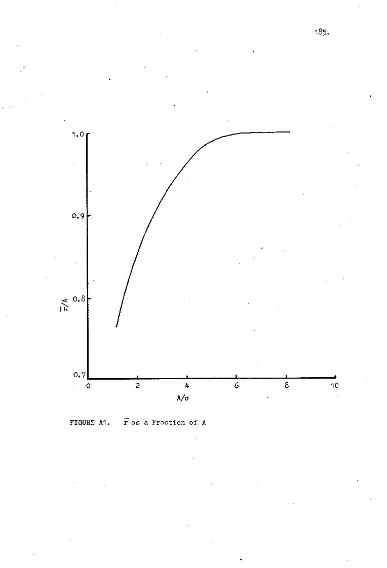
185.

FIGURE Al. r as a Fraction of A

186.

APPENDIX B

COMPUTATION OF SPECTRA USING THE FAST FOURIER-TRANSFORM (FFT)

Because of the finite number of summations which are used in

computations and by its implementation, the fast Fourier transform

(FFT) provides a biased estimate of the power spectrum ( and consequently

the amplitude frequency spectrum ) of a signal. It has been shown by

Oppenheim and Shafer (1975), (pp 541-548), that the estimation of

power spectra using the FFT method is always biased and that the

variance of the estimation does not approach zero as the number of

samples or points is increased. However, a better estimate of the

power spectrum can be obtained by using smoothing or averaging techniques

such as Bartlett's procedure.

One interesting point concerning the estimation of power spectra

using /t.2 routines is that as the number of samples used in the

computation increases, the rapidity of the fluctuations in the spectrum

estimate increases because the uncorrelated frequency samples with zero

covariance move closer together and the variance of the estimated spectrum

approaches a finite, non-zero value (Oppenheim and Shafer, p545).

This fluctuation can be observed in the amplitude frequency spectra

shown in FIGURES 3.1 to 3.6 in Chapter 3. A further example, taken

from Oppenheim and Shafer (p547) is shown in FIGURE B.1. The information

shown in the figure clearly illustrates that the rapidity of fluctuations

in the computed power spectrum increases with increasing numbers of data

samples.

Bartlett's procedure can be used to smooth power spectra and

thereby provide a good estimate of the true spectra. The procedure

consists of taking N samples of data and dividing the N samples into

K groups, each with M samples, such that KM=N. The FFT of each of the

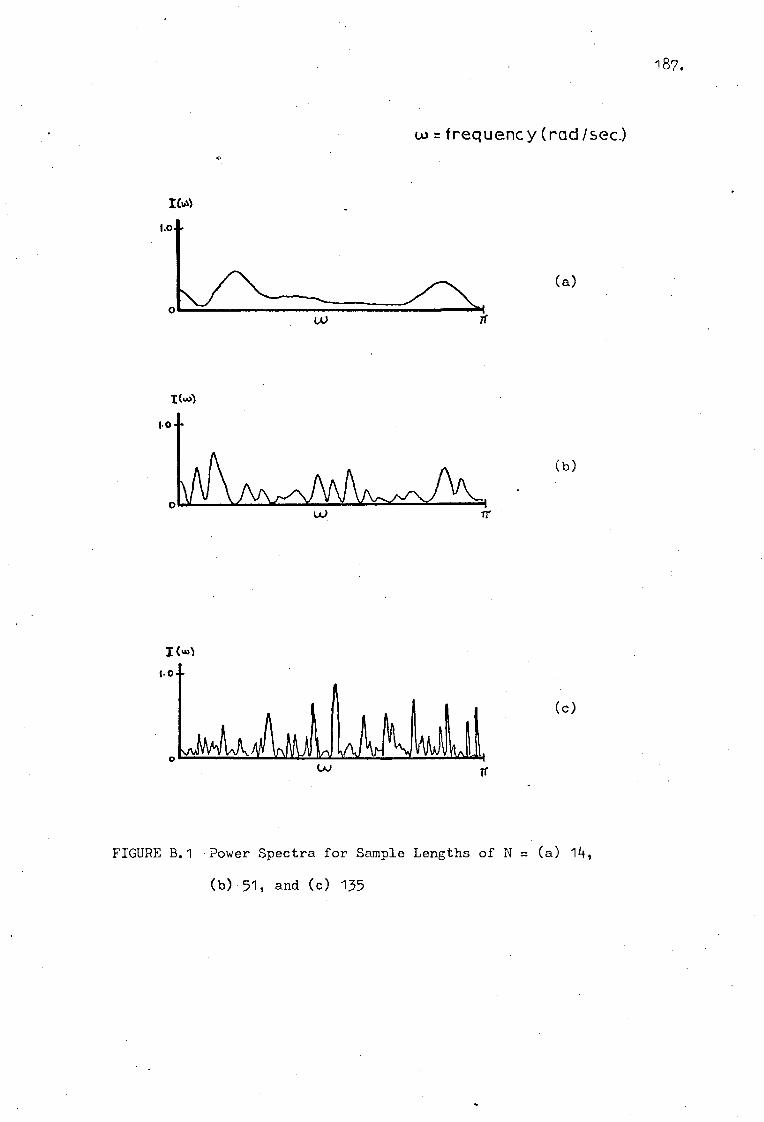
187.

w =frequency (rad /sec.)

(a)

(b)

1. 0

4

0 „AALA. Aka (A)

(c)

FIGURE B.1 Power Spectra for Sample Lengths of N (a) 14,

(b) 5 , and (c) 135

188.

K groups of data is then computed and the K FFTs are added together.

The effect of this operation is, however, to decrease the frequency

resolution in the spectrum when compared to an N-bit FFT. A simple

illustration of this technique is shown in FIGURE B.2 (Oppenheim

and Shafer, p569) in which 14000 samples of data are first divided

into 27 groups, each containing 512 samples,, and then into 280 groups,

each containing 50 samples of data. The effect of this operation is

clearly shown in the figure.

4-,

(a) 2 —

frequency ( rad/sec) 4 .rr

0

co -0

0 7

Ct. E c

4 (b)

frequency ( rad/se )

189.

FIGURE B.2 Power Spectrum Estimates Using Bartlett's Procedure

for N = 14000, and M = (a) 512, and (b) 50

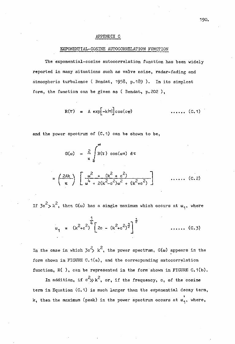
190.

APPENDIX C

EXPONENTIAL-COSINE AUTOCORRELATION FUNCTION

The exponential-cosine autocorrelation function has been widely

reported in many situations such as valve noise, radar-fading and

atmospheric turbulence ( Bendat, 1958, p.189 ). In its simplest

form, the function can be given as ( Bendat., p.202 ),

R(T) = A exp{ cos(c.r) (C.1)

and the power spectrum of (C.1) can be shown to be,

co

G(w) = R(t) cos(wx) dT TE

0

2Ak w2 + (k2 + c2)

w4 + 2(k2-c2)w2 + (k2+c2) (C.2)

If 3c2>lc2, then G(w) has a single maximum which occurs at w1' where

;FL w1 = (k2 - +c2) [2c - (k2+c2)41

(C.3)

In the case in which 3c 2 k2, the power spectrum, G(w) appears in the

form shown in FIGURE C.1(a), and the corresponding autocorrelation

function, R( ), can be represented in the form shown in FIGURE C.1(b).

In addition, if c2 >,>k2 , or, if the frequency, c, of the cosine

term in Equation (C.1) is much larger than the exponential decay term,

k, then the maximum (peak) in the power spectrum occurs at wi, where,

191.

G (co)

(a)

FIGURE C.1 (a) Power Spectrum and (b) Autocorrelation Function

of the Simple Exponential-Cosine Form

192.

4

(c2) (2c - c)1

= c (c.4)

and thus, the peak in the power spectrum occurs at the frequency of

the cosine term in the autocorrelation function.

Although the spectra shown in FIGURES 3.1 to 3.6 are amplitude

frequency spectra, they appear to resemble, in shape, the power

spectrum shown in FIGURE C.1(a). There is also similarity between

the measured autocorrelation functions shown in FIGURES 3.7 to 3.10

and the autocorrelation function shown in FIGURE C.1(b). However,

it is noted that the Fourier transform of the square of Equation (3.1)

is much more complicated than the simple expression given by Equation

(C.1), but the experimental evidence suggests that the spectra and

autocorrelation functions shown in FIGURES 3.1 t 3.10 can be simply

represented by the forms shown in FIGURE C.1.

In FIGURE C.1(b), the times of the first two zero-crossings of

the autocorrelation function are indicated. These times are used

in Chapter 3 to compare the similarity of the autocorrelation

functions and power spectra,which are shown in FIGURES 3.1 to 3.10,

to the simple exponential-cosine form.

193.

APPENDIX D

COMPUTATION OF NOISE SPECTRUM

If white noise is band-pass filtered about a centre frequency,

fo, with an overall bandwidth B, such that B/fo<4,1, then after

envelope detection the baseband noise power spectrum is of the form

( see Rice, 1954 ),

f f = — ( 1 - 73 ) -t- a S (D.1)

where K = constant • 6(0 = unit impulse at the origin

B = overall bandwidth . 2 x baseband bandwidth

The power spectrum given by (D.1) is illustrated in FIGURE D.1.

The total noise power in the band 0 to B Hz is therefore,

2 K (4 - 1) df

Watts (D.2) at = " B/ 2

0

However, in the bandwidth 0 to B/2 Hz, corresponding to the baseband,

the noise power is given by the shaded area in FIGURE D.1, or as,

ap2 i K.B Watts = a2 - t 57 = 7K (D.3)

Thus, the total r.m.s. noise voltage which would be measured in the

band 0 to B/2 Hz is,

ap = Volts (D. 4)

In the computation of the amplitude frequency spectra presented

in Chapter 3, the r.m.s. noise voltage, a , was measured over a

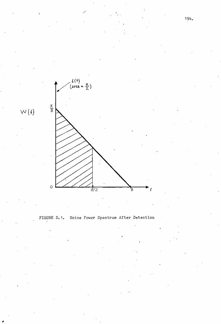
w (+)

194.

FIGURE D.1. Noise Power Spectrum After Detection

•

195.

bandwidth of 4.5 kHz. However, the received signals were then low-

pass filtered at 20 Hz in order to compute the amplitude frequency

spectra. In this narrow band, the noise power spectrum can be

considered to be essentially constant and the noise spectral density

is approximately,

s • W (f) =

K B Watts/Hz (D.5)

Expressed in terms of a , the measured r.m.s. noise voltage, the

noise power spectrum can be written as,

8a2 W (f) = --T

7B (D. 6)

and hence, the amplitude frequency spectrum is given by,

A(f) = 17(7) = 2a PEI p 7B (D.7)

In the tests relating to the measurement of the amplitude frequency

spectra, 0.8 msec duration raised-cosine pulses, repeating every 6.4

msec, were used to modulate a 150 kHz carrier signal. The d.c.

component of such a sequence can be computed as,

1-

1 1h. Sdc = 27( 1 cos(nfT) ) dt

0

= h/16

where h = amplitude of pulse (peak amplitude)

T = duration of pulse in seconds

f = frequency in Hz

(D.8)

196.

The d.c. component of the measured amplitude frequency spectra

can be located in FIGURES 3.1 to 3.6, and thus the noise spectrum

can be drawn in each of the figures, as illustrated. For a peak signal-

to-r.m.s. noise level of 30 dB (typical value), i.e., h/a 30, then

• Sdc

1 7B . 2m 2

A(f)

3o x 9000 32 2

= 166 (D.9)

or, Sdc/A(f) = 44 dB.

Thus, the noise spectrum level is approximately 44 dB below the d.c.

component of the signal spectrum.

From an analysis of FIGURES 3.1 to 3.6, it can be seen that the

computed, approximate, noise spectrum level is well below the levels

of the fluctuation spectra and hence, the effects of background noise

on the fluctuation spectra can be considered to be negligible.

Documents

- AN INVESTIGATION INTO UNDERWATER DATA TRANSMISSION …