2ND LEVEL ANALYSIS AND VULNERABILITY ASSESSMENT OF URM BUILDINGS

Gr.G. Penelis1, A.J. Kappos1, K.C. Stylianidis1 and Ch. Panagiotopoulos1

SUMMARY

A methodology for 2nd level analysis of URM buildings is presented. It includes the estimation of capacity curves for typical building classes, as well as vulnerability (fragility) curves in terms of spectral quantities. The vulnerability assessment methodology is based on a hybrid approach, combining statistical data with appropriately processed results from nonlinear static analyses that permit extrapolation of statistical data to spectral displacements for which no data are available. The data used herein are statistical data from Greek earthquakes, the Thessaloniki 1978 and the Aegion 1995 events, with some additional data from the Pyrgos 1993 earthquake used for comparison purposes. The resulting vulnerability curves correlate spectral displacement to the probability that a building type exceeds a particular damage state.

1. INTRODUCTION

The so-called 2nd level approach for vulnerability analysis involves fragility curves

in terms of spectral quantities (typically displacements); displacements are determined from a convolution of the demand spectrum and the resistance curve of a building. The work on Unreinforced Masonry (URM) Buildings presented herein focuses on two distinct objectives: the development of characteristic (‘prototype’) pushover and capacity curves for typical URM buildings, and the development of vulnerability (fragility) curves using spectral displacement to describe the earthquake input.

Both objectives require a series of nonlinear static analyses of appropriately selected URM building types in order to produce reliable capacity curves as well as to utilise the hybrid vulnerability approach developed by the AUTh team to compensate for the lack of actual (statistical) damage data from a number of earthquake intensities.

2. BUILDING TYPES

The work presented herein refers mainly to simple stone masonry buildings and brick masonry buildings with reinforced concrete floor-slabs, which are by far the most

1 Aristotle University of Thessaloniki (AUTh), Dept. of Civil Engineering, Lab. Of R/C Structures

common types in Thessaloniki, as well as in the rest of Greek cities (see also Penelis et al. 2002). These two main categories are further subdivided into single-storey, two-storey and three-storey buildings.

3. CAPACITY CURVES – STATIC NONLINEAR ANALYSIS

3.1 General A pushover curve is a plot of a building’s lateral load capacity as a function of the

lateral displacement. It is commonly presented as a plot of base shear (preferably normalised with respect to building weight) versus building displacement at roof level (preferably normalised with respect to total building height). Two control points that define a bilinearised pushover curve correspond to the “Yield Capacity” and the “Ultimate Capacity”.

Yield capacity represents the actual lateral strength of the building considering redundancies in design, conservatism in code requirements and actual (rather than nominal) strength of materials. Ultimate capacity represents the maximum strength of the building when the global structural system has reached a fully plastic state (formation of plastic mechanism). Ultimate capacity implicitly accounts for loss of strength due to shear failure of brittle elements. Typically, buildings are assumed capable of deforming beyond their ultimate point without loss of stability, but their resistance to lateral earthquake force is reduced to a degree, which depends on the type of the system; this decrease is generally significant in masonry buildings.

Pushover curves can be converted to so-called capacity curves, based on the equivalent SDOF system approach (see e.g. FEMA 1997); capacity curves are constructed based on estimates of engineering properties that affect the design, yield and ultimate capacities of each model building type. These properties can be defined by the following parameters (Figure 1):

Te true “elastic” fundamental-mode period of building (sec), α1 fraction of building weight effective in pushover mode (represents the mass of

the equivalent SDOF system) α2 fraction of building height at location of pushover mode displacement (effective

height of the equivalent SDOF system) λ “overstrength” factor relating ultimate strength to yield strength, and

µ “ductility” factor relating ultimate displacement to λ times the yield displacement (i.e., assumed point of significant yielding of the structure)

Sa

SdDy DuDd

Au

Ay

Ad

UltimateCapacity

YieldCapacity

DesignCapacity

Fig.1: Capacity curve format

The calculation of prototype pushover and capacity curves is a result of a series of

nonlinear static analyses with several variations in the material properties and the building geometry in order to produce reliable results. 3.2 URM Static Nonlinear analysis – Theoretical background

The method adopted herein for the pushover analysis of URM buildings uses equivalent frame models and concentrated non-linearity at the ends of the structural elements, with a view to simplifying this otherwise cumbersome (for URM buildings) procedure. The non-linearity is simulated with nonlinear rotational springs, whose constitutive law is defined by the moment – rotation curve of each element accounting for both flexure and shear (Kappos, Penelis and Drakopoulos 2002).

For the development of the inelastic Μ-θ curves due to flexure, the following assumptions have been made:

• Zero masonry tensile strength • Parabolic distribution of compression stresses • Bernoulli compatibility (plane sections remain plane) up to failure while the following input data has also been taken into account: • Compressive deformation at failure εο = -2‰ • Compressive strength (fm) of masonry uniform, defined by the strength of bricks

and mortar • Modulus of elasticity Em=550fm (FEMA 1997) The nonlinear shear behaviour has been modelled using a Mohr –Coulomb failure

criterion for the definition of shear strength and a statistical analysis of experimental results for defining shear deformations (Kappos et al. 2002).

The aforementioned methodology has been incorporated in a pre-processor of the commercial software package SAP2000-Inelastic, which allows the pushover analysis of URM buildings. As validation of the results, figures (2a) and (2b) show the analytical simulation of two test cases, a URM wall tested in Pavia (Calvi et al. 1996) and a URM building tested at ISMES, Bergamo.

Theoretical Vs experimental resultsPavia wall D

-150

-100

-50

0

50

100

150

-25 -20 -15 -10 -5 0 5 10 15 20 25

δ [mm]

V (k

N)

Analytical Experimental

Push over curves produced analytically and experimentally

0

0.05

0.1

0.15

0.2

0.25

0.3

0.000 0.005 0.010 0.015 0.020

δ (m)

C (V

/m)

Analytical Experimental

(a) (b)

Fig.2: Analytical simulation of experimental cases (a) Pavia wall (b) ISMES building

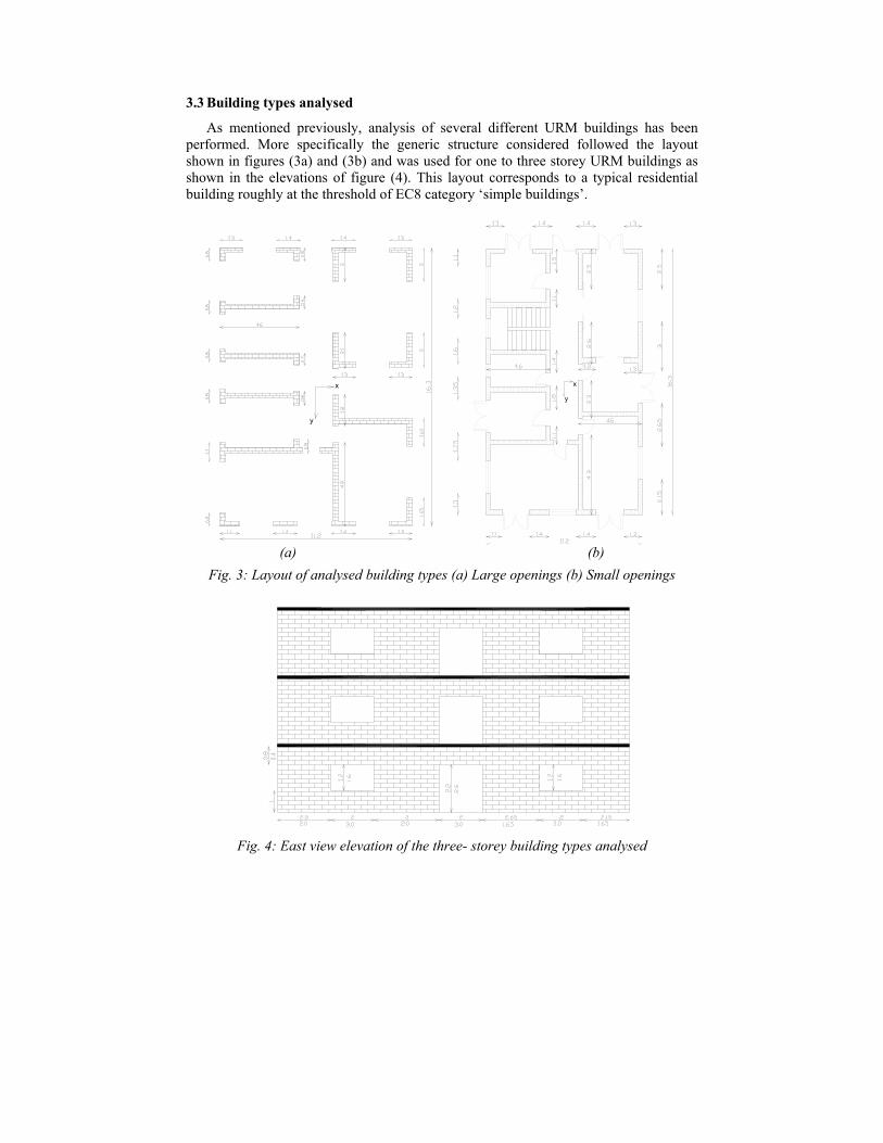
3.3 Building types analysed

As mentioned previously, analysis of several different URM buildings has been performed. More specifically the generic structure considered followed the layout shown in figures (3a) and (3b) and was used for one to three storey URM buildings as shown in the elevations of figure (4). This layout corresponds to a typical residential building roughly at the threshold of EC8 category ‘simple buildings’.

y

x

y

x

(a) (b)

Fig. 3: Layout of analysed building types (a) Large openings (b) Small openings

Fig. 4: East view elevation of the three- storey building types analysed

Two different material properties were used for all the above buildings types: Material A with fwm=1.5 MPa and Material B with fwm=3.0 MPa; for the Young’s modulus E=550fwm was assumed.

All the mentioned variations correspond to thirty six different building types, which were analysed using static nonlinear analysis in order to derive the pushover and capacity curves. 3.4 Results

A total of thirty-six different pushover curves resulted from the analysis of the alternative models considered; these curves, averaged per number of stories, are shown in figure 5 (a). In figures 5(b) and (c) these curves are compared with experimental data from Pavia and ISMES and with the proposed curves in HAZUS (FEMA-NIBS 1999). It is clear that the capacity curves adopted by HAZUS are out of scale in comparison with the curves developed herein, especially those for the low-rise building type. The large discrepancy between HAZUS and our curves lies not in strengths (which are similar if ultimate strength in HAZUS is considered) but in displacements, which are substantially lower in the present analysis, as well as in the tests used for comparison purposes. In table 1 all the analytical features presented graphically in figures 3(a) to 3(c) are presented and compared in a tabular format together with available Italian test data (Calvi et al. 1996, Benedetti et al. 1998) and other proposals (Calvi 1999).

0.000

0.050

0.100

0.150

0.200

0.250

0.300

0.350

0.00% 0.05% 0.10% 0.15% 0.20% 0.25% 0.30%

Drift (%)

Ca

(Vy/

W)

Istorey

2storey

3storey

MEAN

(a)

0

0.05

0.1

0.15

0.2

0.25

0.3

0.35

0 0.0005 0.001 0.0015 0.002 0.0025 0.003

Drift

C=V

/W

2 storey3 storey1 storeyismespavia

0

0.050.1

0.150.2

0.250.3

0.35

0 0.005 0.01 0.015 0.02

Drift

C=V

/W 1 storey2 storey3 storeyismespaviaHAZUS URMLHAZUS URMM

(b) (c)

Fig. 5: Pushover curves and comparison with experimental results and HAZUS curves

Table 1: Comparison of AUTh analytical results with HAZUS, Experiments and Italian data

Period [sec] Experimental Storeys HAZUS99 Calvi et al. AUTh ISMES Pavia

1 0.35 0.123 0.121 N/A N/A 2 N/A 0.153 0.286 N/A N/A 3 0.5 0.233 0.489 N/A N/A

∆y Experimental Storeys HAZUS99 Calvi et al. AUTh ISMES Pavia

1 0.180% 0.100% 0.034% N/A N/A 2 N/A 0.100% 0.053% 0.041% 0.030%3 0.088% 0.100% 0.069% x x

∆u Experimental Storeys HAZUS99 Calvi et al. AUTh ISMES Pavia

1 1.800% 0.300% 0.188% N/A N/A 2 N/A 0.300% 0.241% 0.225% 0.217%3 0.613% 0.300% 0.239% N/A N/A

Ay Experimental Storeys HAZUS99 Calvi et al. AUTh ISMES Pavia

1 0.10 N/A 0.28 N/A N/A 2 x N/A 0.16 0.18 0.31 3 0.08 N/A 0.11 N/A N/A

Au Experimental Storeys HAZUS99 Calvi et al. AUTh ISMES Pavia

1 0.20 x 0.29 N/A N/A 2 x x 0.19 0.22 0.32 3 0.17 x 0.13 N/A N/A

On the basis of table 1, the comment made with respect to figure 5 is further

emphasized, since all suggested values are consistent, except maximum displacements (drifts) suggested by HAZUS which are outliers with regard to both the present analysis and the test data. It is noted that, to the authors’ best judgement, the only factor that was not considered in the analyses (and also in the tests) and could contribute to increased displacements is foundation compliance; this does not explain, though, the afore-mentioned large discrepancies.

In view of the above discrepancies, it is essential to discuss the issue of capacity curves for URM buildings and decide to adopt the values that are more consistent with European data. To facilitate discussion, Fig. 6 is provided, which shows possible idealised envelopes of hysteresis loops resulting from cyclic testing of URM walls critical in shear (Tomazevic & Klemenc, 1997; Magenes & Calvi, 1997). The reported values for the three critical drift values of the trilinear curve (Tomazevic) are as follows:

• at cracking: dcr/h = 0.7÷0.9‰ • at peak load: dHmax/h = 2.2÷2.6‰ • at ultimate: dmax/h = 3.8÷4.4‰

It is noted that drift values at peak load are quite consistent with the calculated values in the present analysis, but significantly lower than the HAZUS values. However, it is also clear that URM structures are characterised by a rather extended post-peak branch (from dHmax to dmax in Fig. 6) and it is well-known that definition of “ultimate” conditions along this branch is always prone to subjective judgement. Referring to the bilinear curve, Magenes and Calvi propose an ultimate drift of 5.3‰, slightly higher than the values from the present analysis (Fig. 5) that does not include post-peak behaviour, but still much lower than HAZUS values.

Trilinear envelope Bilinear envelope

Fig. 6: Idealization of experimentally obtained hysteresis envelope for URM shear walls 3.5 Proposed capacity curves

From the previously presented analyses, capacity curves (in HAZUS format) have been derived for one, two and three storey URM buildings. The corresponding parameters for these curves are given in table 2.

Table 2: Capacity curve parameters URM Buildings Capacity Parameters

BU

ILD

-IN

G

Hei

ght (

m)

Ay (

Cy/W

)

Au (

Cu/W

)

K

[KN

/m)

m

[t]

T (s

ec)

Dy (

mm

)

Du (

mm

)

µ

γ y (%

)

γ u (%

)

1-storey 3.06 0.28 0.29 810907.7 262.4 0.12 1.05 5.76 5.46 0.034 0.188

2-storey 6.19 0.16 0.19 296295.2 524.9 0.29 3.12 14.90 4.78 0.050 0.241

3-storey 9.32 0.11 0.13 155501.4 787.3 0.49 6.40 22.33 3.49 0.069 0.239

MEAN 6.19 0.18 0.20 420901.4 524.9 0.30 3.52 14.33 4.58 0.051 0.223

4. 2ND LEVEL VULNERABILITY CURVES

4.1 General

The 2nd level methodology aims at the calculation of practical expressions, which correlate the earthquake intensity expressed as spectral displacement or acceleration to a descriptor of the building’s damage state (damage level, repair cost, etc). In order to produce vulnerability (fragility) curves that describe more accurately the expected damage for several excitation intensities the hybrid approach has been used herein.

More specifically, the nonlinear analysis presented in section 3 has been combined with the available statistical data from actual events (Thessaloniki, 1978 and Aegion, 1995). 4.2 Hybrid Methodology

The so-called “hybrid” approach to seismic vulnerability (Kappos et al. 1998, Kappos 2001) has been developed in recognition of the fact that reliable statistical data for seismic damage are quite limited and typically correspond to a limited number of intensities.

In Greece, the only reliable damage data available are those from the 1978 earthquake, derived during a previous project (Penelis et al. 1989). Damage data collected in Greece after more recent earthquakes (Kalamata 1986, Pyrgos 1993, Patras 1993, Aegion 1995), although valuable, are generally not in a form that economic damage statistics can be assessed for a representative set of buildings. What usually happens is that the collected data concerns only buildings that have been inspected for a second time (i.e. after the initial post-earthquake rapid screening) and/or wherein some post-earthquake intervention (repair, strengthening, etc.) has taken place; furthermore, the extent of the geographical area (number of municipalities), hence the total building stock to which the data refers, is often unclear.

Unfortunately, even the good quality data for Thessaloniki correspond to a single intensity estimated at about 7 (estimates for the considered area varied from 6.5 to 7.0). It was then clear that either data from abroad should be imported (as often done, especially in relatively low seismicity areas, see Barbat et al. 1996), or the available data should be augmented using either “expert judgement” (see ATC 1985) or an analytical (“mechanical”) approach (see Dolce et al. 1995). Based on the experience from the development and the implementation of the methodology so far, the writers are convinced that purely analytical approaches (such as those adopted in the HAZUS package) should be avoided at all costs, since they might seriously diverge from reality, typically (but not consistently) overestimating the cost of damage.

The basics of the mechanical approach to vulnerability assessment are described in Kappos’ contribution to the EAEE WG3 report (Dolce et al. 1995), while the procedure to apply it for deriving damage probability matrices is described in Kappos et al. (1998). In these publications the emphasis is on methodological aspects (such as the crucial model correlating structural to economic damage index), while application to deriving damage and loss scenarios is of essentially pilot character. Moreover, the analytical component of the method includes inelastic time-history analysis of the response to a number of input motions. In the following, the static nonlinear (pushover) version of the analytical procedure will be presented.

4.3 Damage states

Five different damage levels (states) are proposed herein, defined according to the damage index shown in table 3. The (economic) damage index is the ratio of cost of repair to cost of replacement of a building and it is deemed suitable for vulnerability and loss assessment purposes since it is a “monetary” index.

Table 3: Definition of damage states (levels) Damage level Definition Range of damage index

0 No damage 0 1 Slight damage 0-5 2 Moderate damage 5-20 3 Extensive damage 20-50 4 Very heavy damage & collapse 50-100

To correlate these damage states to an analytical expression of damage, the building

damage index was expressed as a function of yield and ultimate displacement of each building as shown in figure 8; this approach is deemed more versatile than previous ones (e.g. Calvi 1999) based on fixed values of drift ratio for all building types. The analytical expression of the multilinear relationship of figure 8 is shown in table 4. Using these definitions, the expected damage state of a particular building class can be assessed by combining the relevant capacity curve (see §3.5) with the displacement corresponding to a given earthquake intensity.

0.7∆y 0.9∆u

100%

0 %

Displacement

Dam

age

Fig. 8: Damage in URM buildings, as a function of roof displacement

Table 4: Definition of damage as a function of roof displacement Damage level Definition Displacement limits 0 No damage <0.7∆y 1 Slight Damage 0.7∆y<∆<0.7∆y+5(0.9∆u-0.7∆y)/100 2 Moderate damage 0.7∆y+(5(0.9∆u-0.7∆y)/100<

∆<0.7∆y+(20(0.9∆u-0.7∆y)/100 3 Substantial to heavy damage 0.7∆y+(20(0.9∆u-0.7∆y)/100<

∆<0.7∆y+(50(0.9∆u-0.7∆y)/100 4 Very heavy damage 0.7∆y+(50(0.9∆u-0.7∆y)/100<

∆<0.7∆y+(100(0.9∆u-0.7∆y)/100 4.4 Vulnerability Curves

It is well documented in the current literature that such curves can be described by (cumulative) normal, lognormal, beta or other distribution, provided that sufficient data is available. The most common problem when applying a purely empirical approach is the unavailability of (reliable) data for a sufficient number of intensities. By definition, intensities up to 5 lead to negligible damage, particularly cost-wise, therefore gathering of damage data is not feasible, while on the other hand events with intensities 9 or greater are rare, at least for S. Europe, so there are no data available. This unavailability leads to a relative abundance of statistical data in the intensity range from 6 to 8 and a lack of data in the other intensities. This makes the selection of an appropriate

cumulative distribution very unreliable since the curve fit error is significant and the curve shape not as it would be expected.

In order to overcome these problems the following approaches can be followed: • A method could be devised in order to estimate damage at the intensities for which no data is available, by either expert judgement (ATC-13 approach, see ATC 1985) or analytical simulation (AUTh ‘hybrid’ approach, see Kappos et al. 1998). • A purely mathematical, instead of a statistical approach could be adopted in order to fit the desired curve shape to the available data. Within the 2nd level approach, the AUTh team is following the hybrid procedure

since all the required analytical simulations for the hybrid methods have already been carried, while the very nature of the 2nd level approach involves nonlinear analysis. 4.5 Utilisation of available damage databases

Using the information from the Thessaloniki and Aegion databases (see also Penelis et al companion paper in this conference), for deriving damage probability matrices (DPMs) and vulnerability curves, it is essential to firstly define the PGA and spectral displacement assigned to each earthquake.

Based on information reported in the literature (Kappos et al. 1998, Lekidis et al. 1999), the Thessaloniki earthquake gave an intensity 7 in the studied area, while the Aegion earthquake resulted in an intensity of 8 (in the town of Aegion). For both events there are recorder accelerograms that allow the definition of the PGA and spectral displacements, bearing in mind that the PGA is a value that is heavily influenced by the local site and topography conditions at the recording station. The spectral quantities required for level II fragility curves were derived assuming that the spectra of the available records are representative of the ground motion in the corresponding areas.

To establish a link between PGA and intensity (in terms of which empirical data are available) the statistical relationship defined for Greek earthquakes by Theodulidis and Papazachos (1992) was used, which resulted in the PGA values shown in table 5, assumed to characterize on a mean basis the Thessaloniki and Aegion events. It is pointed out that in line with all available expressions of this type, the Papazachos relationship is characterised by a considerable scatter, and this should be kept in mind when using such relationships. In view of this, the PGA values shown in table 5 are quite similar to those actually recorded in the case of Thessaloniki, but about half of those recorded in Aegion; yet, it should not be forgotten that only one record was available from each event, and it did not necessarily represent a “mean” ground motion.

Table 5: Assumed correlation of PGA and intensity Event Intensity Assigned PGA (g)

Thessaloniki 1978 7 0.143 Aegion 1995 8 0.267

In order to evaluate the spectral displacements for the two events, an effective

structural period must be defined; for this purpose the nonlinear static analysis presented in section 3 is utilized, and the mean periods of the three categories are used, i.e. • One storey building T = 0.12 sec

• Two storey building T = 0.29 sec • Three storey building T = 0.48 sec The corresponding spectral displacements for the three categories of buildings and for the two events are shown in table 6.

Table 6: Spectral displacements Sd (mm) for each building type and earthquake Thessal. 1978 Aegion 1995 One storey 0.8 2 Two storey 8 19 Three storey 22 80

4.6 2nd level vulnerability curves in terms of spectral displacement

The standard format of fragility curve used in HAZUS involves spectral displacement. The DPMs corresponding to spectral displacements smaller than the Thessaloniki event were calculated by scaling down the Thessaloniki database, while the ones that correspond to higher than the Aegion event are calculated by scaling up the Aegion database. The scale factor was calculated by using the purely analytical DPMs for all spectral displacements. It is noted that the relation between values in the Thessaloniki and Aegion databases is not constant for single-storey and two-storey buildings since the period is also considered for the determination of the spectral displacement. Moreover, the Sd-based procedure is sensitive to the type of “representative” response spectra selected for each earthquake intensity. Nonetheless, this is a clearly defined procedure, as opposed to the way the HAZUS Sd-based fragility curves are derived.

Using the aforementioned hybrid procedure cumulative DPMs such as those shown in tables 7 and 8 have been calculated for the URM building classes of interest.

Table 7: Cumulative hybrid DPM for two storey stone URM D/Sd [mm] 0.-2.5 2.5-5 5-10 (Thess) 10-15 >15 (Aeg)

0 100% 100% 95% 100% 100%

1 11% 36% 43% 60% 76%

2 0% 19% 29% 58% 58%

3 0% 0% 15% 33% 33%

4 0% 0% 6% 15% 15%

Table 8: Cumulative hybrid DPM for one storey brick URM D/Sd [mm] 0-0.5 0.5-1 (Thess) 1-2 (Aegion) 2-5 >5

0 100% 100% 100% 100% 100%

1 0% 24% 38% 39% 39%

2 0% 15% 29% 29% 29%

3 0% 5% 20% 20% 20%

4 0% 0% 15% 15% 15%

Vulnerability (fragility) curves were then derived by fitting the lognormal cumulative distribution function to the aforementioned cumulative DPMs. The parameters of the lognormal distribution functions were calculated for each building type and damage state and are shown in table 9.

Table 9: Lognormal cumulative distribution parameters for each class STONE 1 STONE 2 BRICK1 BRICK 2

D λ ζ λ ζ λ ζ λ ζ

1 0.277 0.437 2.400 0.800 0.700 0.850 2.700 0.500

2 0.994 0.656 2.800 0.900 1.000 0.800 2.900 0.500

3 1.339 0.564 3.200 0.700 1.300 0.700 3.100 0.500

4 1.783 0.385 3.400 0.600 1.500 0.650 3.500 0.650

Using these parameters, the fragility curves shown in figures 9 and 10 are plotted. Alternative curves in terms of PGA have also been derived using again the hybrid approach and are presented elsewhere (Penelis et al. 2002).

2nd Level vulnerability curves for 1storey Stone URM Buildings

0

10

20

30

40

50

60

70

80

90

100

1 2 3 4 5 6 7 8 9 10 11 12

Sd [mm ]

P(D

>DS/

Sd)

1

2

3

4

ACT1

ACT2

ACT3ACT4

2nd Level vulnerability curves for 2storey Stone URM Buildings

0

10

20

30

40

50

60

70

80

90

100

3 8 13 18 23 28 33 38 43 48

Sd [mm]

P(D

>DS/

Sd)

1

2

3

4

ACT1

ACT2

ACT3

ACT4

Fig.16: Lognormal cumulative distribution curves for one and two storey stone URM

2nd Level vulnerability curves for 1storey Brick URM Buildings

0

10

20

30

40

50

60

70

80

90

100

0.5 1.5 2.5 3.5 4.5 5.5 6.5 7.5 8.5 9.5 10.5 11.5

Sd [mm]

P(D>

DS/S

d)

1

2

3

4

ACT2

act3

ACT4

ACT1

2nd Level vulnerability curves for 2storey Brick URM Buildings

0

10

20

30

40

50

60

70

80

90

100

3 8 13 18 23 28 33 38 43 48

Sd [mm]

P(D

>DS/

Sd)

1

2

3

4

ACT1

ACT2

ACT3

ACT4

Fig.17: Lognormal cumulative distribution curves for one and two storey brick URM

5. CONCLUSIONS

The methodology adopted for the development of the 2nd level analysis of URM buildings has been presented herein. The work included two independent phases: the definition of capacity curves for URM building typologies common in Greece and the definition of 2nd level vulnerability (fragility) curves correlating spectral displacement to the probability of a building type to exceed a particular damage state, using a hybrid methodology which combines actual statistical data collected from past earthquakes with inelastic analysis for the intensities for which there are no data available. The purely statistical data used are from Greek earthquakes, the Thessaloniki 1978 and the Aegion 1995 events, with some additional data from the Pyrgos 1993 earthquake.

The results presented herein include capacity curves (in HAZUS format) for single-storey and two-storey URM buildings of either stone or brick masonry. Moreover, using the aforementioned hybrid approach, new fragility curves for standard URM building classes have been constructed, in terms of spectral displacement. These are based both on a limited number of analyses (12 for each class), and on a limited number of ground motion (Thessaloniki 1978 and Aegion 1995 records), hence they should be further checked and verified.

REFERENCES ATC, 1985. Earthquake damage evaluation data for California (ATC-13). Appl. Technology

Council, Redwood City, Calif. Barbat, A.H. et al., 1996. Damage Scenarios Simulation for Seismic Risk Assessment in

Urban Zones, Earthquake Spectra, 12(3), 371-394. Benedetti, D., Carydis, P., and Pezzoli, P., 1998. Shaking table tests on 24 simple masonry

buildings, Earthquake Engineering & Structural Dynamics, 27(1), 67-90. Braga, F., Dolce, M., Liberatore, D., 1982. Southern Italy November 23, 1980 Earthquake: A

Statistical Study on Damaged Buildings and an Ensuing Review of the M.S.K.-76 Scale. CNR-PFG n.203, Roma.

Calvi, G. M., 1999. A displacement-based approach for vulnerability evaluation of classes of buildings, Journal of Earthquake Engineering, 3(3), 411-438.

Calvi, G.M., Kingsley, G.R., and Magenes, G., 1996. Testing of Masonry Structures for Seismic Assessment, Earthquake Spectra, 12 (1), 145-162.

Dolce, M., Kappos, A., Zuccaro, G. and Coburn, A.W., 1995. State of the Art Report of W.G. 3 - Seismic Risk and Vulnerability, 10th European Conference on Earthquake Engineering, Vienna, Austria (Aug. - Sep. 1994), Vol. 4, 3049-3077.

Dolce, M., Marino, M., Masi, A. and Vona, M., 2000. Seismic vulnerability analysis and damage scenarios of Potenza, Proceed. International Workshop on Seismic Risk and Earthquake Scenarios of Potenza (Potenza, Italy, Nov. 2000), pp. 35-56.

Fardis, M.N., Karantoni, F. V., and Kosmopoulos, A., 1999. Statistical evaluation of damage during the 15-6-95 Aegio Earthquake, Final Report to the Sponsor (EPPO, Athens), Patras (in Greek).

FEMA, 1997. NEHRP Guidelines for the Seismic Rehabilitation of Buildings, FEMA-273, Washington D.C., Oct. 1997.

FEMA-NIBS, 1999. Earthquake loss estimation methodology - HAZUS99 Technical Manual, Volumes 1-3, Washington DC.

Kappos, A.J., 2001. Seismic vulnerability assessment of existing buildings in Southern Europe, Keynote lecture, Convegno Nazionale “L’Ingegneria Sismica in Italia” (Potenza/Matera, Italy), CD ROM Proceedings.

Kappos, A.J., Pitilakis, K.D., Morfidis, K. and Hatzinikolaou, N., 2002. Vulnerability and risk study of Volos (Greece) metropolitan area, 12th European Conference on Earthquake Engineering (London, UK), CD ROM Proceedings (Balkema), Paper 074.

Kappos A.J., Penelis, Gr.G., and Drakopoulos, C., 2002. Evaluation of simplified models for the analysis of unreinforced masonry (URM) buildings, Journal of Structural Engineering, ASCE, Vol. 128, No. 7, 890-897.

Kappos, A.J., Stylianidis, K.C., and Pitilakis, K., 1998. Development of seismic risk scenarios based on a hybrid method of vulnerability assessment. Natural Hazards, 17(2): 177-192.

Karantoni, F. V., Bouckovalas, G., 1997. Description and analysis of building damage due to Pyrgos, Greece earthquake, Soil Dynamics & Earthquake Engineering, 16(2), 141-150.

Lekidis, V.A., et al., 1999. The Aegio (Greece) seismic sequence of June 1995: Seismological, strong motion data and effects of the earthquakes on structures, Journal of Earthquake Engineering, 3(3), 349-380.

Lekkas, E., Fountoulis., I. and Papanikolaou, D., 2000. Intensity Distribution and Neotectonic Macrostructure Pyrgos Earthquake Data (26 March 1993, Greece), Natural Hazards 21(1): 19–33.

Magenes, G., and Calvi, G.M., 1997. In-plane seismic response of brick masonry walls, Earthquake Engineering and Structural Dynamics, 26(11), 1091-1112.

Papazachos, B. and Papazachou, C., 1997. The Earthquakes of Greece, Ziti Editions, Thessaloniki.

Penelis, G.G., Sarigiannis, D., Stavrakakis, E. and Stylianidis, K.C., 1989. A statistical evaluation of damage to buildings in the Thessaloniki, Greece, earthquake of June, 20, 1978. Proceedings of 9th World Conf. on Earthq. Engng., (Tokyo-Kyoto, Japan, Aug. 1988), Tokyo:Maruzen, VII:187-192.

Penelis, Gr.G., Kappos, A.J., and Stylianidis, K.C., 2002. WP4 – 2nd level analysis: Unreinforced masonry buildings, RISK-UE working document, May.

Penelis, Gr., Kappos, A., Stylianidis, K., & Lagomasino, S., 2002. Statistical asssessment of the vulnerability of URM buildings, International Conference on Earthquake Loss Estimation and Risk Reduction, Bucharest, Romania.

Theodulidis, N.P. and Papazachos, B.C., 1992. Dependence of strong ground motion on magnitude-distance, site geology and macroseismic intensity for shallow earthquakes in Greece: I, Peak horizontal acceleration, velocity and displacement, Soil Dynamics and Earthquake Engineering, 11, 387-402.

Tomazevic, M. and Klemenc, I., 1997. Seismic behaviour of confined masonry walls, Earthquake Engineering & Structural Dynamics, 26(10), 1059-71.