Embed Size (px)
Citation preview
-Ai8S 458 TRACTION MODEL DEVELOPMENT(U) MRC BEARIMGS-SKF 1/2AEROSPACE ICING OF PRUSSIA PR J I RCCOOL SEP 87AFMAL-TR-97-4079 F33615-84-C-5928
UNCLASSIFIED F/G 11/B U
EEEEomhEEmomiIEhmhohEEmhhhhE

11IL
U. 11Q6u I
MICROCOPY RESOLUTION NEST $HART
AFWAL-TR-87-4079 FILE uub
0In
TRACTION MODEL DEVELOPMENT
00
I J. I. McCool
SMRC Bearings-SKF AerospaceTribonetics1100 First AvenueKing of Prussia PA 19406-1352
September 1987
Final Technical Report for Period: 28 September 1984 - 31 March 1987
Approved for public release; distribution is unlimited
DTICS ELECTEDEC0 9S8
MATERIALS LABORATORYAIR FORCE WRIGHT AERONAUTICAL LABORATORIESAIR FORCE SYSTEMS COMMANDWRIGHT-PATTERSON AIR FORCE BASE OH 45433-6533
UNCLASSIFIEDSECURITY CLASSIFICATION OF THIS PAGE A
REPORT DOCUMENTATION PAGEis REPORT 3ECURITY CLASSIFICATION lb. RESTRICTIVE MARKINGS
UNCL.ASSIFIED None2s. SECURITY CLASSIFICATION AUTHORITY 3. DISTRIBUTION/AVAI LABILITY OF REPORT
___________________________________ Approved for public release; distribution2b. DECLASSIFICATION/DOWNGRADING SCHEDULE is unlimited.
4. PERFORMING ORGANIZATION REPORT NUMBER(S) 5. MONITORING ORGANIZATION REPORT NUMBER(S)
NA AFWAL-TR-87-4079
6a. NAME OF PERFORMING ORGANIZATION ~b. OFFICE SYMBOL 7a. NAME OF MONITORING ORGANIZATION
%MRC BEARINGS-SKF AEROSPACE (1if pt.abWe Air Force Wright-Aeronautical LaboratoriesMaterials Laboratory (AFWAL/MLBT)
6c. ADDRESS (City. State and ZIP Code) 7b. ADDRESS (City, State and ZIP Code)
1100 First Avenue Wright-Patterson AFB, OH 45433-6533Kinci of Prussia PA 19406-1352
So. NAME OF FUNDING/SPONSORING Sb. OFFICE SYMBOL 9. PROCUREMENT INSTRUMENT IDENTIFICATION NUMBER
I F33615-84-C-5028
S& ADDRESS (City. State and 711' Ctd..) 10. SOURCE OF F UNDING NOS.
PROGRAM PROJECT TASK WORK UNITELEMENT NO NO. NO. NO
11 TITLE fInctude Security Classification) 62102F 2421 01 36* ~Traction Model Development ______ ________________
12. PERSONAL AUTHOR(S) .-
13.. TYPE OF REPORT 13b. TIME COVERED 7;7TBF:EOR YrMo ;7u) 15. PAGE COUNTFnlFROM 840928 TODT FREOT(, 163
16. SUPPLEMENTARY NOTATION
17. COSATI CODES Is. SUBJE jT )$ S (Continue on reverse if necesary and identify by block number)
FIELD GRIOUP suB. GR.V
9 Traction, Modelling, Traction Model
19. ABSTRA VConlinue on reverse of necessary and identify by block number)
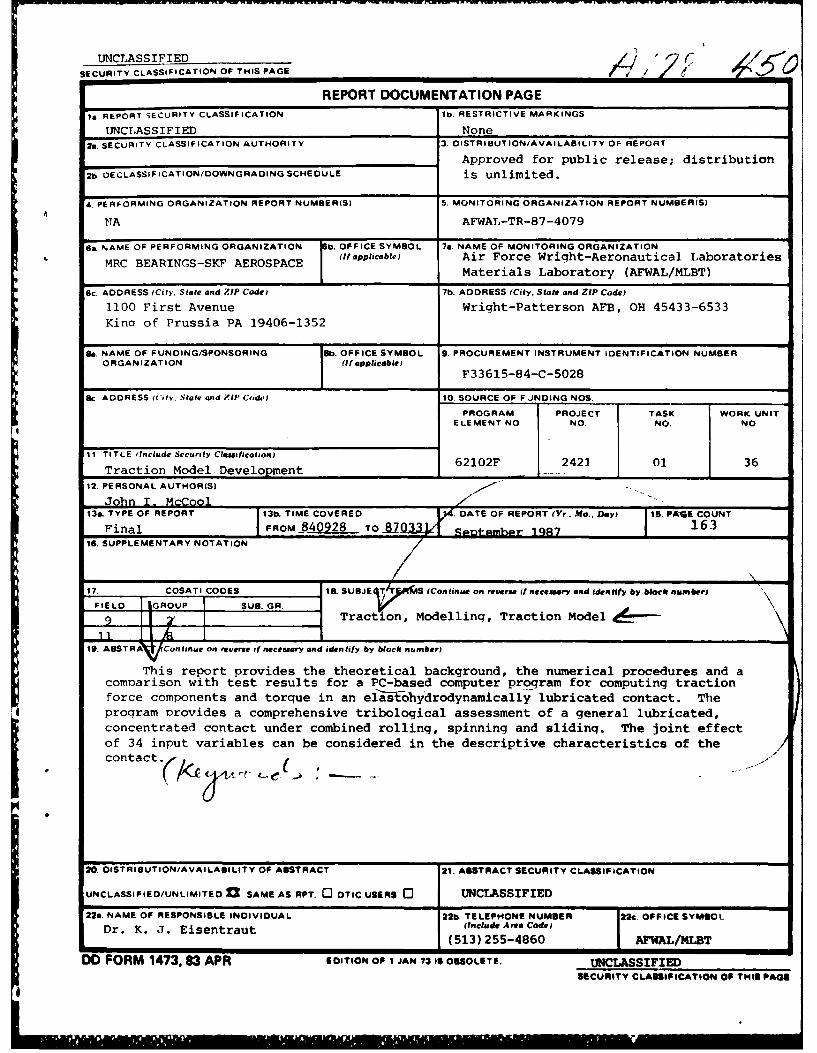
This report provides the theoretical background, the numerical procedures and acomoarison with test results for a PC-based computer proqran for computing tractionforce components and torque in an efas-tah3drodynamically lubricated contact. Theproqram Drovides a comprehensive tribological assessment of a general lubricated,concentrated contact under combined rolling, spinning and slidinq. The joint effectof 34 input variables can be considered in the descriptive characteristics of the
* contact.(
20. OISTRIBUTION/AVAILABILITY OF ABSTRACT 21. ABSTRACT SECURITY CLASSIFICATION
UNCLASSI FIE D/UNLIMITEO0 0 SAME AS RPT. 0 OTIC USERS 0 UNCLASSIFIED
22a. NAME OF RESPONSIBLE INDIVIDUAL 22b. TELEPHONE NUMBER 22c. OFFICE SYMBOL
Dr. K. J. Eisentraut (include Area Code)(513) 25-80AFWAL/MLBT
DD FORM 1473, 83 APR EDITION OF I JAN 73 IS OBSOLETE. UNCLASSIFIEDSELCURITY CLASSIFICATIOIN OF THIS PAGEI

TABLE OF CONTENTS
PAGE
1.0 INTRODUCTION.............................. 12.0 PROBLEM STATEMENT........ . . ................ 83.0 FILM SHAPE, CONTACT DIMENSIONS AND
PRESSURE DISTRIBUTION. . .. . .. . . . ................. 16
3.1 Film Shape ................................... 163.1.1 Fully Flooded Central Film Thickness ......... 183.1.2 Starved Central Film Thickness*,,***......... 193.1.3 Film Reduction Due to Inlet Heating .......... 203.2 Contact Ellipse Dimensions and Pressure ...... 213. 3 Pressure Shift. . . .. . . .. .. . . .. .. . . .. . . o. 253.4 Deborah Number..o....... ... .. ......... .. .... o. 27
4.0 ASPERITY CONTACT TRACTION MODEL AND SURFACEFATIGUE INDEX..o.....o....o........................ 29
4.1 The Greenwood-Williamson MicrocontactModel....... ........ o...ooo........ o....... o.. 30
4.2 Fatigue Ine...... ........... 324.3 Relating the GW Parameters to Spectral
4.4 Estimating m4 from Stylus ProfileEquipment Otu......................... 37
4.5 Expected Values of Traction ForceComponents and Torque at Asperities.......... 40
5.0 RHEOLOGICAL MODEL FOR FLUID TRACTIONooo ... o.oo.... 44
5.1 One-Dimensional Maxwell Model.. ... ....... 445.2 Nonlinear One-Dimensional Maxwell Model...... 465.3 The Trachman-Cheng Nonlinear Viscous Model... 485.4 The Nonlinear One-Dimensional Maxwell
Model Using the Trachman-Cheng Viscous
5.5 Application to aLine Contactoosoooooooeooooo 49
6.0 SOLUTION SCHEME FOR CONSTITUTIVE EQUATIONS.... o..... 57
7.0 HEAT GENERATION AND THERMAL ANALYSIS... o....... 64
7ol Heat Generation...... . . . .. .. . .. .. . .. .. 6407.1.1 Fluid Shear Heat... 90060009090009999990040660 64 07.1.2 Heat Generated at Asperities.....006......... 657.*2 Thermal Aayi....................... 657o2.1 Temperature Distribution in Solid and Film... 657o2.2 Temperature and Pressure Dependence of
Lubricant Properties. . . . . . .. .. . .. .. . .. 68.;;y Codes
r i.'dor
iii ,5
TABLE OF CONTENTS (Concluded)
PAGE
8.0 PROGRAM DESCRIPTION, ORGANIZATION, LOGIC FLOW ANDUSERS INFORMATION. . . .. .. . . .. . . .. ................ 73
8.1 Description of Computer Program...........6 738.2 Program Organization.............. 748.*3 Program Logic Flow.. 999999 *ooo~o. . .. .. 748.4 User's Information.....*..*****.....oo..... 818.4.1 Installing the Program..o................... 818.4.2 Executing the Program... ........o............ 838.4.3 Creating an Input Data Fie.........83
9.0 TRACTION TEST PROGRAM....99999999 9 0
9.1 Traction Rig and Test Variables...... ... .... 1019.2 Lubricant Selection.ooososooooso 1oo03
9.4 Further Lubricant Properties... ....... .ooll 11
9.4.2 Temperature Viscosity Coefficient...o.......1129.4.3 Pressure Viscosity Coefficient..ee*...e.*.1129.4.4 SpecificGrvt..... . .... ..... 139.4.5 Conductivityoo. . .... . 999,,, ... 99..1149.*4.96 SpecificHet * . ... 9.** * .14
9. 5 TestDein ...... ...... . .. 15
10.0 TRACTION DATA REDUCTION, ANALYSIS AND DISCUSSION.... 119
10.1 Traction Data Base. ............. 99.9000*9.99.911910.*2 Predicted Traction Curves. . .. o~****e*9 12810.3 Viscoplastic Regime. 999999999999999.99oo.999913510.4 The Trachman-Cheng Viscous Model**.........4410.5 Alternative Approach to Speeding
Convergence Rate.. .. 99**e.***. *9*ee.... 14610.6 Estimating Gand TC66.96*.6..................150
REFERENCES..999*9...9.9.9.9999..99999 9.......... * 5
iv

LIST OF FIGURES
FIGURE NO. PAGE
2.1 MOVING BODIES IN DRY CONTACT ................. 9
2.2 FILM SHAPE AND PRESSURE DISTRIBUTION ......... 112.3 ASPERITY CONTACTS THROUGH PARTIAL
OIL FILM ..................................... 13
3.1 EHD FILM SHAPE AND INLET MENISCUSGEOMETRY ..................................... 17
3.2 PRINCIPAL PLANES & RADII FORCONTACTING BODIES .............. .............. 22
3.3 IDEALIZED EHD CONTACT GEOMETRYAND KINEMATICS WITH SHIFTEDPRESSURE DISTRIBUTION .......... ............. 26
4.1 RELATION BETWEEN SUMMIT AND SURFACEMEAN PLANES. .... ... ...... . ..... ......... .... 35
5.1 /ic VS. DIMENSIONLESS STRAIN RATE........... 525.2 T/Tc VS. DIMENSIONLESS STRAIN RATE W/T....... 53
6.1 CONTACT ELLIPSE COORDINATE SYSTEM............. 58
7.1 SURFACE AND FILM TEMPERATURE PROFILES........ 67
8.1 OVERALL FLOW DIAGRAM FOR PROGRAMMCFRIC .... . ................................ . 76
8.2 LOGIC DIAGRAM FOR SUBROUTINE TRACT........... 788*2.1 THERMAL ANALYSIS....... .... ................. 808.3 INPUT FILE - SAMPLE.DAT ...................... 848.4 MCFRIC OUTPUT FOR FILE SAMPLE.DAT............ 89
9.1 AFML TRACTION RIG ............................ 1029.2 EXPERIMENTAL TRACTION CURVE................. o1049.3 A TYPICAL TRACTION CURVE...................107
10.1 TRACTION FORCE VS. SLIDING SPEEDAFML FILE NO. K18FOP1 ........................ 129
10.2 TRACTION FORCE VS. SLIDING SPEEDAFML FILE NO. K07B1V9.............. .......... 130
10.3 TRACTION FORCE VS. SLIDING SPEEDAFML FILE NO. K1809V7........ ............. o..131
10.4 TRACTION FORCE VS. SLIDING SPEEDAFML FILE NO. M18N9GO.......................132
10.5 TRACTION FORCE VS. SLIDING SPEEDAFML FILE NO. K1809V7........................133
10.6 TRACTION FORCE VS. SLIDING SPEEDAFML FILE NO. M18N9GO. ............. ........ 134
10.7 TRACTION FORCE VS. SLIDING SPEEDAFML FILE NO. L28H7P1 .............. .......... 136
10.8 TRACTION FORCE VS. SLIDING SPEEDAFML FILE NO. L088B4W0.....,.................137
v

LIST OF FIGURES (Concluded)
FIGURE NO. PAGE
10.9 TRACTION FORCE VS. SLIDING SPEEDAFML FILE NO. Ll7H9Pl ........................*138
10.10 TRACTION FORCE VS. SLIDING SPEEDAFML FILE NO. Ll7H9P1 ........................1l39
10.11 TRACTION FORCE VS. SLIDING SPEEDAF!4L FILE NO. t18EV7 ............ *...........140
10.12 TRACTION FORCE VS. SLIDING SPEEDAFML FILE NO. M18EOV7 ............ *v***ee*#*..145
10.13 TRACTION FORCE VS. SLIDING SPEEDAFML FILE NO. M18EOV7 ............ *...........149
vi
LIST OF TABLES
TABLE NO. PAGE
8.1 MODULES, FUNCTIONS AND SUBROUTINENAMES FOR McFRIC ............................ 75
9.1 ADJUSTED TRACTION DATA POINTS ............... 105
9.2 TRACTION DATA TEST MATRIXMOBIL RL-714 ...................... o ... .... 116
9.3 TRACTION DATA TEST MATRIXSANTOTRAC-50 ................... ... so.... . 117
9.4 TRACTION DATA TEST MATRIX HF-CTFE ........... 118
10.1 TRACTION DATA FORM ................. .......121
10.2 MOBIL RL-714 DATABASE ....................... 122
10.3 SANTOTRAC-50 DATABASE ...................... 124
10.4 HF-CTFE DATABASE ................ . .... 126
vii
1.0 INTRODUCTION
This report provides the theoretical background, the numeri-
cal procedures, a user's description and a comparison with test
results for a PC based computer program for computing traction
force components and torque in an elastohydrodynamically, lubri-
cated contact. The program is dubbed McFRIC because it was
designed primarily to compute FRICtion, including the effect of
MicroContacts. The program in fact provides a comprehensive tri-
bological assessment of a general lubricated, concentrated con-
tact under combined rolling, spinning and sliding. It reflects
the joint effect of 34 input variables in computing the following
descriptive characteristics of the contact:
1. The contact ellipse dimensions and area.
2. The elastohydrodynamic (EHD) film thickness both at the
plateau and at the constriction that forms at the rear
of a lubricated, concentrated contact under fully
flooded (unstarved) and isothermal lubricant inlet con-
ditions.
3. A film thickness correction factor accounting for a
viscosity decrease of the oil in the contact inlet due
to shear heating.
4. A film thickness correction factor accounting for lubri-
cant starvation in the contact inlet.
1
5. The apportionment of the applied load between the
asperities and the lubricant film, using the
Greenwood-Williamson microcontact model with parameters
estimated from the ordinary output of a stylus profile
device.
6. The estimated mean square curvature of the composite
surface roughness profile, the density of surface sum-
mits and the mean asperity tip radius.
7. The mean number of asperity contacts and the real con-
tact area, i.e., the total contact area of the elasti-
cally deformed asperities.
8. The average number of microcontacts which have undergone
plastic flow within the contact area at the computed
surface separation.
9. An index of surface fatigue behavior based on the number
and area of plastic microcontacts.
10. The magnitude of the spin torque and the magnitude and
direction of the tractive force transmitted between the
contacting bodies by the combined effects of (i)
shearing of the fluid film and (ii) coulomb friction
OA_ between contacting asperities. This computation may be
performed isothermally or thermally. With the thermal
option the heat generated by both types of interfacial
2

friction raises the temperature of the fluid film and
the surfaces and alters the lubrica :t properties. The
computed torque and force components are printed and
optionally plotted as a function of sliding velocity in
the rolling direction.
11. The average and maximum value of the temperature of the
lubricant film and the surfaces, when the thermal option
is elected.
12. The power transmitted by the contact and the power
dissipated in friction. This is printed and optionally
plotted as a function of sliding speed.
Section 2.0 is a narrative outline of the scope of the trac-
tion prediction problem as it is addressed in this report.
Section 3.0 is a summary of the computational procedures used
for computing the thickness of the lubricant film separating the
contacting bodies, accounting for the effects of lubricant film
starvation and inlet heating. The relationships employed to com-
pute the dimensions of the contact ellipse, the total elastic
approach of the contacting bodies, and the contact pressure are
summarized.
Section 4.0 is a description of the methodology employed to
calculate the load sharing between the pressurized lubricant film
and the elastically deformed surface asperities which penetrate
3
it. The analysis yields the density of microcontacts, the mean
real and mean apparent pressure due to asperity deformation, the
density of plastic microcontacts, and the mean real elastically
deformed area of contact. These quantities are computed as func-
tions of the plateau film thickness and the RMS profile height
and slope of the two contacting bodies using the assumption that
the surface roughness processes are isotropic and that the
spectrum of the composite roughness is a power function of spa-
tial frequency. The computation of the asperity contribution to
the total traction torque and force components is developed
postulating coulomb friction at the microcontacts.
Section 5.0 is a description of a nonlinear Maxwell rheologi-
cal model adopted for computing fluid traction. The
Trachman-Cheng constitutive law is used as the nonlinear viscous
component. It is shown how the model is capable of accounting
for viscous, elastic and plastic fluid behavior as appropriate.
The numerical scheme used to solve for the components of the
fluid shear stress as a function of the position within the con-
tact ellipse is outlined in Section 6.0. The fluid viscosity is
taken to vary with pressure in accordance with Barus' equation.
The fluid's limiting shear strength is taken to be proportional
to pressure. Both of these fluid properties are therefore spa-
tially variable over the contact ellipse via the Hertzian distri-
bution of pressure. The integration of the shear stress
4
components over the contact ellipse to yield the traction force
components, torque and power loss is also described.
The iterative analysis whereby the steady state solid and
film mean plane temperatures are computed is described in Section
7.0. Fluid shearing and asperity friction combine to form the
heat source. This heat is dissipated by the mechanisms of con-
duction and convection. The analysis accounts for the mean
effect of temperature in the film on the lubricant viscosity and
limiting shear strength.
The organization and logic flow of McFRIC is given in Section
8.0 along with a detailed description of the iterative thermal
solution. This section contains instructions for installing the
program and for the preparation of input data. A sample program
input file and the corresponding program output are given.
Section 9.0 contains a description of the traction tests con-
ducted at AFML including lubricant selection, specimen and test
rig description the choice of test variables and the specific
test matrices used for each lubricant.
Lubricant specific rules for the computation of six physical
properties as a function of temperature are described for each of
the three test fluids. Computation of the limiting shear
strength of the fluid and of the shear modulus of the composite
system comprising the lubricant and the near surface layers of
the contacting bodies, is discussed.
5

Reduction of the traction test data and the compilation of a
traction data base is described in Section 10.0. These data are
used as input to McFRIC in an effort to predict the experimental
traction curves. The data showed that the thermal effect was
A. overpredicted when the limiting shear strength was taken to vary
inversely with absolute temperature. With this dependence
removed the relatively minor thermal effects exhibited by the
data were well explained with a thermally dependent viscosity.
Fits were found to be acceptably good for all cases in which
the Deborah number computed at the mean Hertzian pressure via
Barus' Law exceeded unity. This included all of the data for two
of the oils and roughly half of the data for the third. For the
cases in which the Deborah number was less than unity the pre-
dicted curves approached their asymptotic value with increasing
strain rate too slowly. An approach is adopted for these cases
of using an empirical viscosity value to bring the prediction
into accord with the experimentally observed traction curve slo-
pes. This approach though successful is shown to be equivalent
to simply increasing the Deborah number. It is suggested that
the Trachman-Cheng model may need to be supplemented with a
further lubricant dependent parameter that governs the speed of
convergence to the limiting shear strength as shear rate
increases.
In the concluding part of Section 10.0 regression fits to the
limiting shear strength and elastic modulus values for the three
6
oils are listed. Using these approximate equations one may use
McFRIC for conditions of load, speed, contact ellipse aspect
ratio and temperature for which traction tests are not available.
Numerous contributions were made in the early stages of this
work by Gail Hadden and Lea Sheynin. Robert Aman compiled the
traction data base and authored the program MATPROP. Mark Ragen
converted McFRIC to run on a PC and developed the input data
structure. He also provided the information for program users
given in Section 8.0. John Walsh and Monica Friday conducted
most of the McFRIC runs and reruns and performed the data
plotting. Advice and many valuable suggestions offered in tech-
nical discussions with Dr. Luc Houpert of SKF during the course
of this work, are gratefully acknowledged.
7
2.0 PROBLEM STATEMENT
The subject being addressed herein is the lubricated contact
of two moving elastic bodies, focusing on the problem of pre-
dicting the resultant forces and torque due to the tangential
stresses distributed over their interface.
The forces are known as friction or traction forces; the
torque as spinning moment or spinning torque.
The bodies are assumed to be bounded by surfaces of revolu-
tion with their separation in the vicinity of a point of defor-
mationless contact, assumed to be adequately approximable as a
second degree polynomial in a system of coordinates having its
origin at the contact point. With this assumption, and in the
absence of a lubricant, the equations of Hertz apply for the
calculation of 1) the mutual approach of the bodies under a load
P 2) the dimensions a and b respectively, of the semimajor and
semiminor axes of the elliptical interfacial contact area and 3)
the elliptically paraboloid distribution of interfacial normal
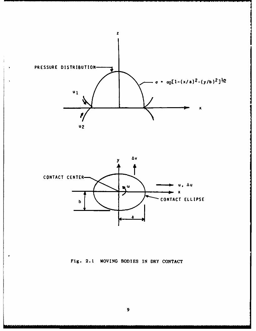
pressure. Figure 2.1 shows the contact and relevant velocities
and dimensions. The two surfaces are presumed to move with
respective velocities uI and u2 in a direction coincident with
one of the principal axes of the contact ellipse. The average
velocity in that direction is denoted u = (ul + u2)/2. u is
customarily termed the rolling or longitudinal velocity. The
difference Au = ul - u2 is known as the sliding or slipping
velocity.
8
z
PRESSURE DISTRIBUTION- -i
o *oo(1-(x/a)2-(y/b) 2 l2
x
u2
CONTACT CENTER
Il -u UU
x
b ~~ CONTACT ELLIPSE
a
Fig. 2.1 MOVING BODIES IN DRY CONTACT
9

Av denotes the velocity difference in the direction orthog-
onal to u. It is known as the transverse sliding velocity or side
slip. Finally, a relative rotational velocity known as spin may
act about an axis perpendicular to the contact ellipse and through
its center.
Figure 2.1(b) shows the distribution of interfacial pressure
and its equation expressed in an orthogonal coordinate system
established at the contact center and with the x-axis coincident
with the semimajor axis of the contact ellipse. This pressure
integrates over the contact area to a force equal to the applied
normal force P.
If a viscous lubricant is introduced and adheres to the sur-
faces as they approach the converging inlet to the contact region,
a fluid pressure builds and, for the class of fluids typically
used as lubricants, the viscosity increases and the surfaces
separate and deform to allow the fluid to pass through the con-
tact region or 'nip' as it is referred to in some literature.
Figure 2.2 shows the consequences of the introduction of the
lubricant on the dry contact pressure distribution and shape of
the gap between the contacting bodies. The pressure distribution
is extended forward in front of the dry contact ellipse. The gap
is relatively flat except for a constriction near the exit end of
the contact. A large 'spike' in the pressure distribution pre-
cedes the exit constriction as shown.
10

Typical lubricant pressure
rycontact pressure
Surface No.2 I
r - Dry contactSurface No. IA
Fig. 2.2 FILM SHAPE AND PRESSURE DISTRIBUTION
The exact thickness and slope of the lubricant film is deter-
mined by the joint solution of the Reynold's equation of hydrody-
namics and the deformation equations of contact elasticity. The
film separating the surfaces is consequently known as an elasto-
hydrodynamic (EHD) film.
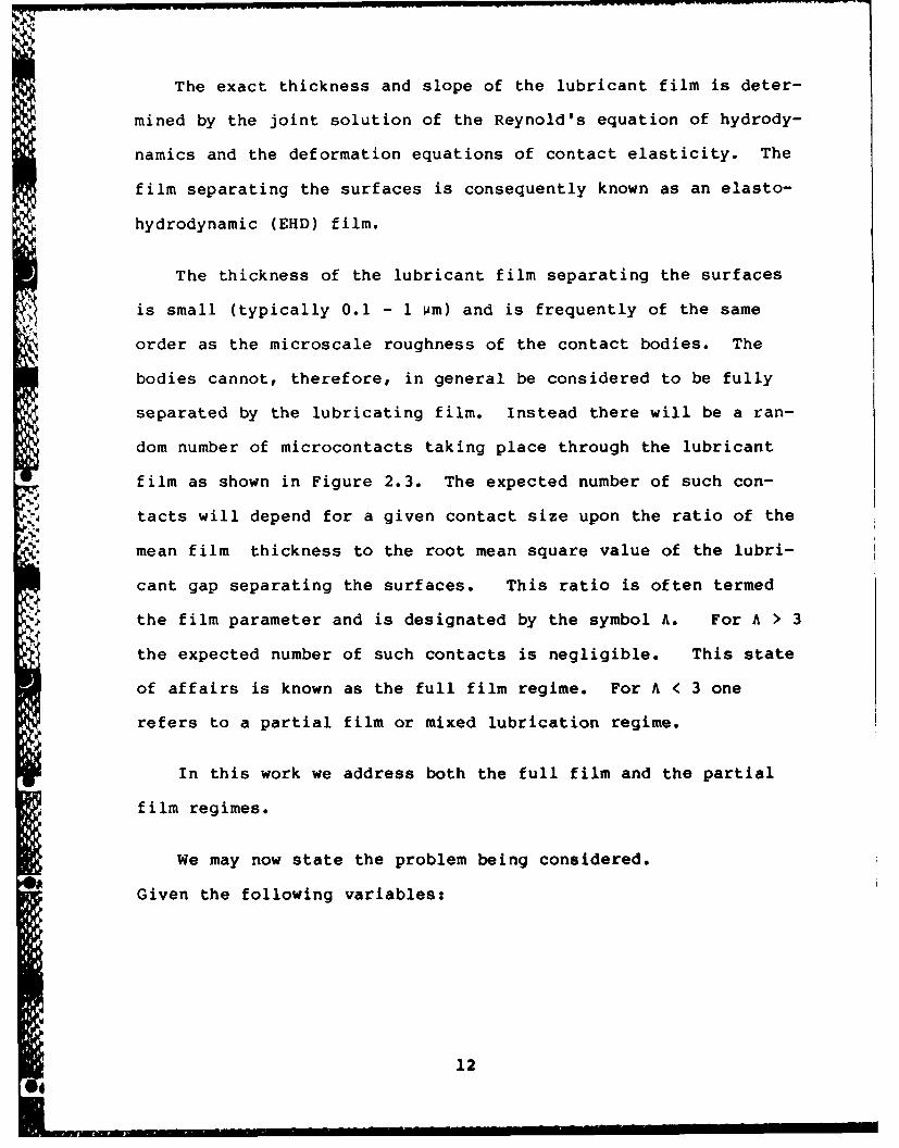
The thickness of the lubricant film separating the surfaces
is small (typically 0.1 - 1 Pm) and is frequently of the same
order as the microscale roughness of the contact bodies. The
bodies cannot, therefore, in general be considered to be fully
separated by the lubricating film. Instead there will be a ran-
dom number of microcontacts taking place through the lubricant
film as shown in Figure 2.3. The expected number of such con-
tacts will depend for a given contact size upon the ratio of the
mean film thickness to the root mean square value of the lubri-
cant gap separating the surfaces. This ratio is often termed
the film parameter and is designated by the symbol A. For A > 3
the expected number of such contacts is negligible. This state
of affairs is known as the full film regime. For A < 3 one
refers to a partial film or mixed lubrication regime.
In this work we address both the full film and the partial
film regimes.
We may now state the problem being considered.
Given the following variables:
124
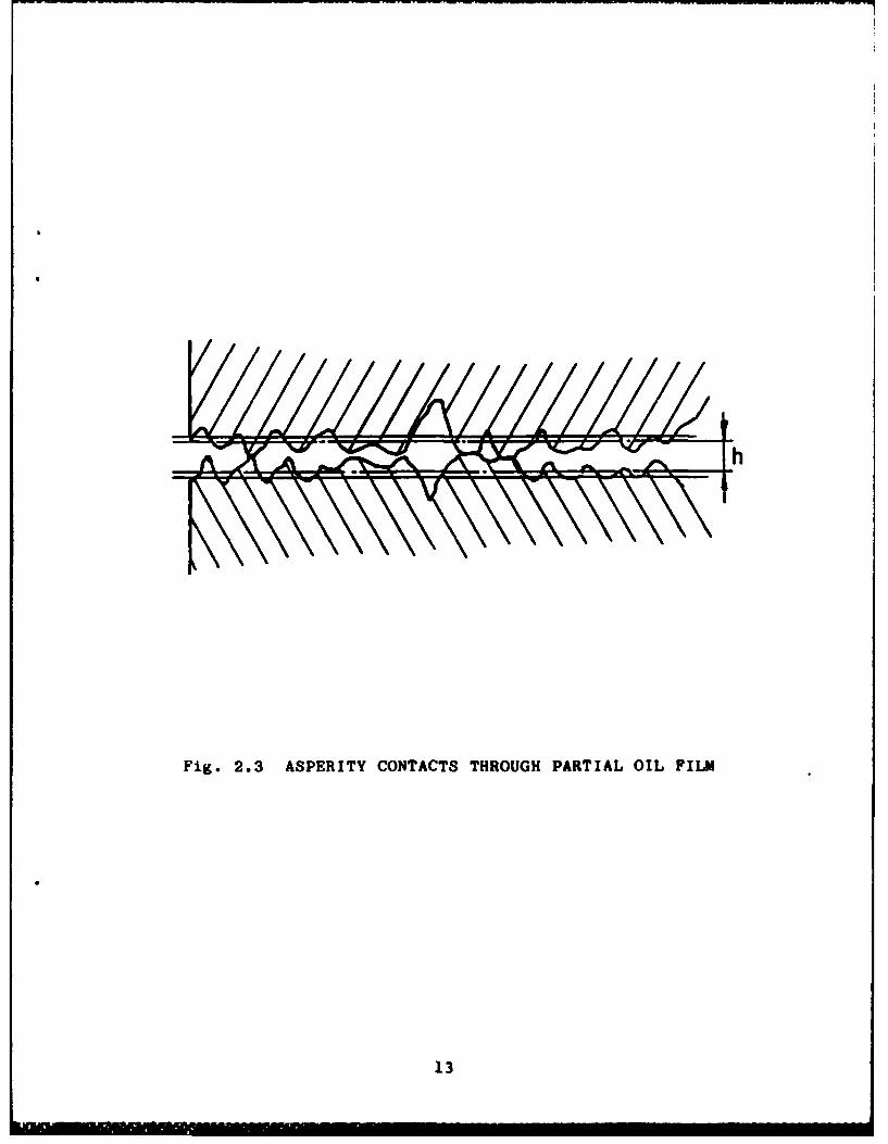
Fig. 2.3 ASPERITY CONTACTS THROUGH PARTIAL OIL FILM
13
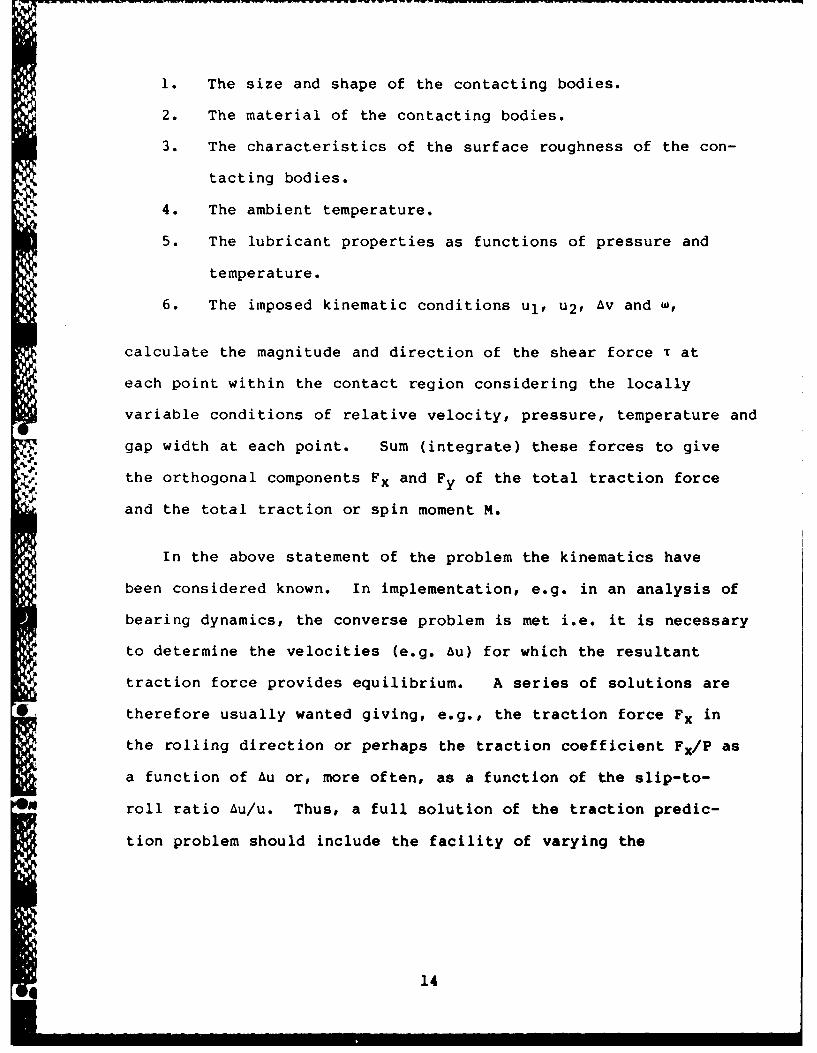
1. The size and shape of the contacting bodies.
2. The material of the contacting bodies.
3. The characteristics of the surface roughness of the con-
tacting bodies.
4. The ambient temperature.
5. The lubricant properties as functions of pressure and
temperature.
6. The imposed kinematic conditions uI, u2 , Av and w,
calculate the magnitude and direction of the shear force T at
each point within the contact region considering the locally
variable conditions of relative velocity, pressure, temperature and
gap width at each point. Sum (integrate) these forces to give
the orthogonal components Fx and Fy of the total traction force
and the total traction or spin moment M.
In the above statement of the problem the kinematics have
been considered known. In implementation, e.g. in an analysis of
bearing dynamics, the converse problem is met i.e. it is necessary
to determine the velocities (e.g. Au) for which the resultant
traction force provides equilibrium. A series of solutions are
therefore usually wanted giving, e.g., the traction force Fx in
the rolling direction or perhaps the traction coefficient Fx/P as
a function of Au or, more often, as a function of the slip-to-
roll ratio Au/u. Thus, a full solution of the traction predic-
tion problem should include the facility of varying the
14
kinematics systematically and calculating the associated traction
force components and spinning moment.
The solution of the traction prediction problem involves
making the appropriate choice of a relationship between the
conditions at each point (pressure, relative velocity, tem-
perature, gap thickness, etc.) and the shear stress and in
deducing the constants and properties which are embodied in that
relationship.
1
15

3.0 FILM SHAPE, CONTACT DIMENSIONS AND PRESSURE DISTRIBUTION
In this section the method adopted for the computation of key
variables which affect the solution of the traction prediction
problem is outlined. These variables are 1) the thickness and
shape of the lubricant film that separates the surfaces, 2) the
* shape and dimensions of the interfacial contact area between the
- surfaces and 3) the magnitude, shape and location of the inter-
facial pressure distribution.
3.1 Film Shape
As noted, the introduction of lubrication has the effect of
separating the contacting surfaces by a film of virtually
constant thickness over a central plateau region while pro-
viding a somewhat smaller film separation over a narrow constric-
tion that forms at the rear of the contact. As is customary in
traction calculations, the film shape will be taken to be
constant with thickness equal to the computed plateau thickness.
Highly accurate solutions for the plateau film thickness have
been developed by Hamrock and Dowson [i for the fully flooded
condition where a copious lubricant supply is available and for
the 'starved' case where the lubricant meniscus is at a finite
distance Xb, forward of the contact center as shown in Figure
3.1. The value of Xb responds to the method of lubricant supply.
By specification of Xb it will be possible for the user of the
16

(b)
117
traction model to account quantitatively for the effect of lubri-
cant supply rate on the traction condition. Heating in the inlet
will increase the inlet temperature above ambient, thus lowering
the viscosity and hence the EHD film. A multiplicative reduction
factor is used to account for this effect as discussed below:
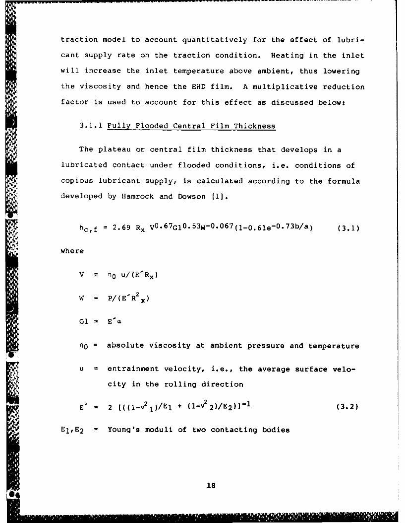
3.1.1 Fully Flooded Central Film Thickness
The plateau or central film thickness that develops in a
lubricated contact under flooded conditions, i.e. conditions of
copious lubricant supply, is calculated according to the formula
developed by Hamrock and Dowson [1].
hcf = 2.69 Rx VO.67G1O.53W-0-0 67 (l-0.61e-0.73b/a) (3.1)
where
V = n0 u/(E'Rx)
W = P/(E'R2 x )
GI = E'Q
no = absolute viscosity at ambient pressure and temperature
u entrainment velocity, i.e., the average surface velo-
city in the rolling direction
E' = 2 [((I-v 21 )/El + (I-v2 2)/E 2 )]-1 (3.2)
EI,E 2 = Young's moduli of two contacting bodies
18

vl,v 2 = Poisson's ratio for the two contacting bodies
Rx = effective radius in rolling direction
S= pressure viscosity coefficient
a,b = contact ellipse semi-axes in the direction of and
transverse to the rolling direction
This formula was developed by curve fitting to the results
obtained in full computer solutions of the equations of elastic-
ity and hydrodynamics. The results were obtained for cases with
b > a, i.e. with the contact ellipse major axis transverse to
the rolling direction but, as stated by Hamrock and Dowson,
remain plausible for a > b.
3.1.2 Starved Central Film Thickness
The starved central film thickness hc,s is calculated by
multiplying the fully flooded central thickness hc,f by the
'starvation' factor s,c. Os,c is computed as
M1 0.29o s,c = (Xb/a-1) ] Xb/a < m* (3.3)
(m*- )
= 1.0 Xb/a > m*
m*= 1 + 3.06 [(Rx/a) 2 (hc,f/Rx)]0 . 5 8 (3.4)
19
0
Formulas comparable to Eqs. (3.1) and (3.3) have been deve-
loped for the constriction film thickness as well. These are
also incorporated in McFRIC and the constriction film thickness
is printed for reference.
3.1.3 Film Reduction Due to Inlet Heating
Convergence of the lubricant film in the EHD contact inlet
results in heating of the inlet oil with a consequent loss in
viscosity and thinning of the lubricant film. Murch and Wilson
[21 have analyzed this problem and derived a multiplicative fac-
tor t which may be applied to the isothermally calculated film
*to correct for this effect. The factor is given by
.t = 1/(l + 0.108A0 . 6 2 ) (3.5)
where
A = 4n 0 Ou2/k (3.6)
and
k = heat conductivity of the oil
0 = temperature viscosity coefficient (°R)-I defined through
Reynold's viscosity-temperature relation
n = no e-O(T-T0)
T = temperature
20
I IZ
no viscosity at temperature To and ambient pressure
u = entrainment velocity
3.2 Contact Ellipse Dimensions and Pressure
The calculation of elastic contact ellipse dimensions and the
contact pressure follows classical Hertzian theory [3].
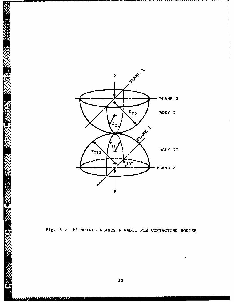
Figure 3.2 shows the assumed undeflected forms and dimensions
of the bodies that comprise the type of contacts that are being
considered. Prior to deflecting under the load P, the boundaries
of the bodies in the vicinity of contact are surfaces of revolu-
tion. The principal planes, i.e., the orthogonal planes in which
the radii of curvature are largest or smallest are assumed to
coincide. The principal radius for Body I in Plane 1 is denoted
ril. Correspondingly, the principal radius for Body II in Plane
1 is denoted r I . The principal radii in Plane 2 are denoted
r1 2 and r1 1 2 , respectively.
Under the action of the load P, the surfaces will deflect and
the region of contact will expand from a point to an elliptical
area. The axes of the contact ellipse will be parallel to the
principal planes. Whether the major axis of the contact ellipse
is parallel to Plane 1 or to Plane 2 depends upon the relative
magnitudes of the principal radii.
It is possible to consider a somewhat more general contact
situation in which the principal planes for Bodies I and II make
21
P 4
PLANE 2
BODY 11
- PLANE 2
P
Fig. 3.2 PRINCIPAL PLANES & RADII FOR CONTACTING BODIES
22
an arbitrary angle with each other. However, inasmuch as the
most complete state-of-the-art film thickness and fluid traction
models assume that the rolling direction is parallel to one of
the axes of the contact ellipse, we limit consideration to the
geometry of Figure 3.2.
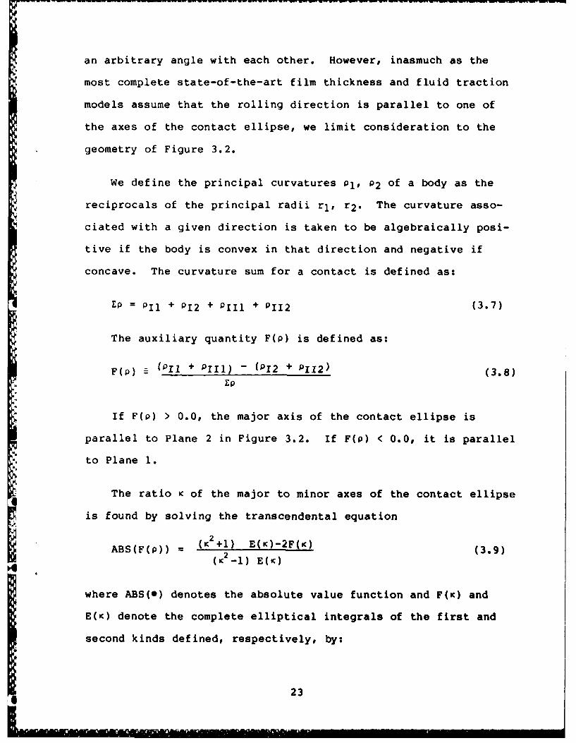
We define the principal curvatures Pl, P2 of a body as the
reciprocals of the principal radii rI, r2. The curvature asso-
ciated with a given direction is taken to be algebraically posi-
tive if the body is convex in that direction and negative if
concave. The curvature sum for a contact is defined as:
EP = PIl + P12 + P I I + PII2 (3.7)
The auxiliary quantity F(p) is defined as:
F()E (PI1 + P ill) - (P12 + P112)(38F(p) a I' - +(3.8)
If F(p) > 0.0, the major axis of the contact ellipse is
parallel to Plane 2 in Figure 3.2. If F(p) < 0.0, it is parallel
to Plane 1.
The ratio K of the major to minor axes of the contact ellipse
is found by solving the transcendental equation
ABS(F(p)) (2 +1) E(K)-2F(K) (3.9)(K2-1) E(K)
where ABS(e) denotes the absolute value function and F(K) and
E(K) denote the complete elliptical integrals of the first and
second kinds defined, respectively, by:
23
F( K) [ I [ - -2)sin 2 ]-/2 dP (3.10)
0
and
([= 1- [-K(-1/2)sin2,]1/2 dp (3.11)0
The major axis kI may be calculated as
6K 2 E(K) p)1/ 3 (3.12)
E EP
where
P = applied load
[ L-.E 12 -1 reduced elastic modulus
EI,1 I = elastic moduli of Bodies I and II
I, II = Poisson's ratio
The minor axis is computed as
X2 = a/K (3.13)
The contact area A is
A = 1T £lt2 (3.14)
The total distance 6 through which remote points within the
contacting bodies move under the action of the load P, is
6 = F(K) 0 [9(EP) (P/1KE') 2 ]I/3 (3.15)2E(K)
The maximum pressure o0 acting on the contact ellipse is
o = 1.5 P/A (3.16)
,. 24
4NOMOO
The average pressure p is simply,
p = P/A (3.17)
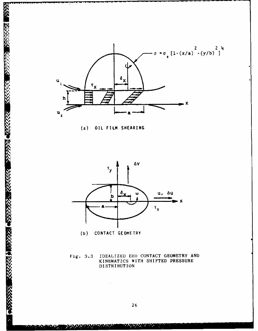
3.3 Pressure Shift
As noted, the presence of the lubricant redistributes the
interfacial pressure from its dry contact, Hertzian, shape.
Tevaarwerk and Johnson [4] suggested that to a first approxima-
tion this effect could be modelled as a forward shift 6x of the
dry contact pressure distribution. The dry contact center still
serves as the axis of spin since that is kinematically deter-
mined.
The displacement 6x of the load center due to the redistribu-
tion of Hertzian pressure by the lubricant film as shown in
Figure 3.3, is calculable by the formula developed by Hamrock and
cited in Tevaarwerk and Johnson (4].
6x = 4.25 a (gl)0 .022 (g 2 )-0. 3 5 (b/a)0 -9 1 (3.18)
where gl and g2 are the following dimensionless variables:• €,p3
p 3 =(3.19)
n 0 u E Rx
P 2/Y 2 3 (3.20)
As noted, the magnitude of the contact ellipse dimensions and
pressure distribution are calculated using the Hertz equations.
-' 4 2 5
2 2
u2
(a) OIL FILM SHEARING
1AV
-O x
(b) CONTACT GEOMETRY
Fig. 3.3 IDEALIZED Elit) CONTACT GEOMETRY ANDKINEMATICS WITH SHIFTED PRESSUREDI STRIBFUTION
26
Figure 3.3 shows the shifted pressure distribution and inter-A
facial area over which the shear stresses are appreciable.
3.4 Deborah Number
As discussed in depth below in Section 5.0, the Deborah
number plays a key role as a determinant of whether a fluid beha-
ves viscously or elastically as it deforms under sliding con-
ditions. For an isoviscous fluid, the Deborah number is defined
as
T = nu/aG (3.21)
where n, u and a as defined previously are the viscosity, entrain-
.ment velocity and contact ellipse semi axis in the rolling direc-
tion. G is the shear modulus of the elastic composite formed by
the fluid and the contacting bodies.Sq-
Inasmuch as the viscosity varies with pressure through the
contact, the Deborah number is a point function of the spatial
coordinates within the contact region. To compute a represen-
tative number one could use a value of the viscosity averaged by
means of an appropriate pressure viscosity law over the contact
pressure distribution. As a simple approach in computing the
Deborah number, the average viscosity is approximated as the
viscosity at the average pressure computed using the Barus rela-
*tion. That is,
27
= rlo e Up (3.22)
where p, the average pressure is
p = 2/3 o (3.23)
and 'lio is the viscosity at ambient pressure.
If the Barus' equation applies over the full contact, the
average viscosity will substantially exceed the viscosity com-
puted in this manner. Nevertheless the value thus computed is
indicative, in that it responds to changes in pressure and
ambient viscosity. Quantitative interpretation of T, i.e.,
classifying fluid behavior based on the value of T is discussed
in Section 10.0.
28
4.0 ASPERITY CONTACT TRACTION MODEL AND SURFACE FATIGUE INDEX
As indicated in Section 2.0, considering the partial EHD
regime brings the added complexity of asperity contact into the
traction prediction problem. Bair and Winer [5) show curves of
traction force against the film parameter A, in which a six fold
increase of traction occurs as A decreases from 1.0 to 0.3.
Clearly the role of asperity contact cannot be ignored.
The approach taken within program McFRIC is to use the
Greenwood-Williamson (GW) microcontact model [6] to determine the
average force acting at a contacting asperity, the number of
microcontacts per unit area and the real contact area as a func-
tion of the apparent area. A summary of the GW model is given in
Section 4.1 below.
The three GW model parameters are deduced in terms of the
RMS height and RMS slope using the spectral estimation approach
proposed by McCool [7]. This method is summarized in Section
4.3.
Assuming that coulomb friction with a known friction coef-
ficient acts at the deformed asperities the statistical expec-
tation of the net traction force components and torque is
computed as described in Section 4.4.
29

4.1 The Greenwood-Williamson Microcontact Model
The Greenwood-Williamson microcontact model applies tr the
contact of a rough surface and a smooth plane. It is based on
the assumptions that:
1. Asperities have spherically capped summits of constant
radius R irrespective of their height.
2. Asperities are mechanically independent, i.e. the load
they support depends on their height and not upon the
load supported by neighboring asperities.
3. Asperities deform elastically in accordance with the
. Hertzian relations between deflection, load and contact
area.
4. Summit height expressed as a deviation from the mean
plane of the summits is a random variable and follows a
gaussian probability distribution with standard
deviation as .
Comparisons of the Greenwood-Williamson model with more
comprehensive models that relax many of its seemingly restrictive
assumptions, show that it is nonetheless astonishingly accurate
in its predictions (8]. In view of this and its simplicity to
use, it has been adopted as the microcontact model for use within
McFRIC.
30
The GW model requires three input parameters:
DSUM : the surface density of summits
.. as : the standard deviation of the probability distribu-
tion of summit heights and
R : the deterministic (non-random) radius of the spheri-
cal summit caps.
Given the values of these parameters, the contact density
ZNCON, the total asperity supported force TOTF, the total real
area of contact per unit nominal area, TOTA, and the average
asperity supported force AVF, are computed as:
ZNCON = DSUM 0 F0 (d/Os ) (4.1)
TOTA = N DSUM R OS Fl(d/Gs ) (4.2)
TOTF = 1.333 A0 DSUM E' R1/2 Gs3/2 F3/2 (d/as ) (4.3)
and
AVF = 1.333 EORI/ 2 as3/2 F3/2 (d/as)/F 0 (d/os) (4.4)
The density Np of plastic contacts, i.e., of contacts which
have experienced some degree of subsurface plastic flow is given
by
Np - DSUM * F0 (d/os + Wp*) (4.5)
The elastically computed microcontact area, Ap, of the
plastically deformed contacts, per unit nominal area A0 , is given
by:
Se 31

Ap/AO DSUM 0 F1 (d/Gs + Wp*) (4.6)
where
E' = [(I-v 2 1)/E l + (1-v 22 )/E2 - (47)
EIE 2 Young's modulus for the rough and smooth surfaces
vl,v 2 = Poisson's ratios for the rough and smooth surfaces
Wp * = 6.4R(Y/E' )2/os G8)
Y = Yield strength of rough surface in simple tension
O Fo(O),Fl(*),F 3/ 2 (*) = Functions defined in terms of the standard
gaussian density function. Values are
tabled e.g. in [8]. Piecewise approxima-
tions to these functions are employed
within McFRIC.
4.2 Fatigue Index
If the microcontact area is denoted A, the number of plastic
contacts acting over this area, ZNPLAS, is given by:
ZNPLAS = Np 0 A (4.9)
The mean area APLAS of a plasticized asperities is
APLAS = Ap/Ao * A/ZNCON (4.10)
An index of fatigue behavior P, proposed in [19], is the
product of the number and average area of plastic contacts i.e.,
04 32

= ZNPLAS 0 APLAS (4.11)
It is reasoned that the higher the value of 0, the greater
the opportunity for surface initiated fatigue failure. No stu-
dies have yet been performed to quantify the relation between
fatigue life and 4. It is nonetheless a reasonable index to use
to gauge relative performance of a number of surface/lubricant
combinations.
4.3 Relating the GW Parameters to Spectral Moments
In work subsequent to the development of Greenwood and
Williamson's model, it was found that the GW parameters could be
expressed in terms of 3 quantities, m 0 , m 2 and m4 , known as
spectral moments. These values may be determined from a profile
z(x) as
m 0 = AVG (z2 (x)) (4.12)
m 2 = AVG [(dz(x)/dx) 2 (4.13)
m 4 = AVG [(d2 z(x)/dx 2 ) (4.14)
where z(x) represents the profile height deviation from the sur-
face mean plane at some position x, relative to an arbitrary ori-
gin. m 0 is, of course, Rq 2 and is frequently called a2 in the
Tribology literature. m 2 is the mean square slope and m 4 is,
very nearly, the mean square curvature.
Under the assumption that z(x) is a gaussian random variable
the summit density, DSUM, is given by Longuet-Higgins [9) as
330++ r + ... .. IlbIII iiiii
DSUM = (m 4 /m 2 )/6 13"- (4.15)
Bush et al [101 suggest that the radius R may be approximated as
the reciprocal of the average summit curvature and give the
expression
R = 0.375 (t/n 4)1/2 (4.16)
Bush et al also express the summit height standard deviation
as as
s = (1-0.8968/a)1/2 m 01/2 (4.17)
where C, termed the bandwidth parameter, is defined as:
I2- (m0m4 )/m2
2 (4.18)
It is more usual in Tribology to use the profile mean plane
as a reference than the summit mean plane used by the GW model.
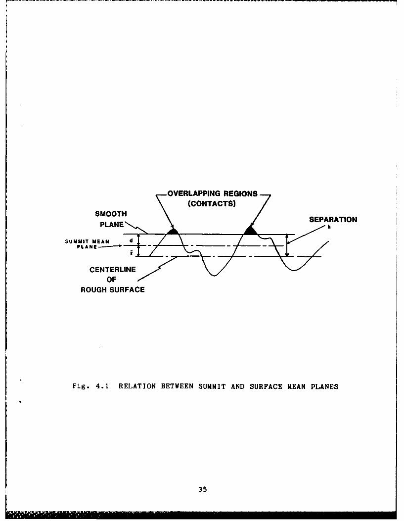
Figure 4.1 shows that a smooth surface whose height above the sum-
mit mean plane is d, is situated at a distance h = d + - above
the profile mean plane. The difference in mean planes is
expressible as (Bush et al [10])
z = 4(mo/ic)I/ 2 (4.19)
Using Eqs. (4.17) and (4.19) the film parameter A i.e., the ratio
h/Rq 2 h/a is found to be linearly related to d/a s as:
d/a s = [(h/a) - 4/(wr)I/ 2 ]/(1-0.8968/a)l/ 2 (4.20)
34
OVERLAPPING REGIONSX (CONTACTS)
SMOOTHSEPARATION
CENTERLINEOF
ROUGH SURFACE
Fig. 4.1 RELATION BETWEEN SUMMIT AND SURFACE MEAN PLANES
35
For a specified h/a value and given values of mo, m2 and N4 ,
one may use Eq. (4.20) to find d/as and thereafter, Eqs. (4.1) to
(4.4) to compute the microcontact conditions at that h/a value.
When both surfaces are rough an equivalent smooth and rough sur-
face is considered in which the values of m0 , m2 and m4 are
summed for the two rough surfaces, i.e.:
m0 = (mO)l + (mO)2 (4.21)
m2 = (m2)1 + (m2)2 (4.22)
m4 = (m4) 1 + (m4) 2 (4.23)
where (mn)i denotes the n-th spectral moment for profile i
(i=1,2). The mn values computed from Eqs. (4.21) to (4.23) are
referred to as composite values. When surfaces are anisotropic
there exist two orthogonal directions, called principal direc-
tions, along which the profile value of m2 is a minimum and a
. maximum. According to [11], the value of m2 , designated (m2)e,
for an equivalent isotropic surface may be constructed as the
harmonic mean:
(m2)e = (m2max * m2min )1/2 (4.24)
The m4 values in the same two principal directions are com-
bined in the same way to give (m4)e. In principle m0 is inde-
pendent of tracing direction. If m0 is measured in two
directions along with m2 and m4, the ordinary arithmetic average
and not the harmonic mean should be used to combine the two
values of m0 .
36
4.4 Estimating N4 from Stylus Profile Equipment Output
As shown above, the GW model is completely specified if we
know m0 , m2 and N4 for the composite and for the equivalent
isotropic surface. These quantities may be computed directly
from a profile as the finite difference approximations to Eqs.
(4.12) to (4.14). Alternatively, m0 , m2 and N4 may be computed
in terms of the spectrum s(f) of a profile if the spectrum is
known or estimated. Roughly speaking the spectrum is a function
that expresses how the various frequencies present in a random
profile contribute to the overall profile variability.
It has been found empirically that the spectrum of a rough-
ness profile most always plots nearly linearly on a set of
logarithmic scales with perhaps spikes at frequencies which
correspond to the spacing of grinding furrows, chatter or other
nearly periodic features. It is postulated, therefore, that the
spectrum is of the form s(f) - f-k where k, termed the spectral
exponent, is the magnitude of the slope of a plot of log s
against log f. Introducing a proportionality constant 'c' gives
s(f) = cf-k (4.25)
It is further postulated that the spatial frequencies present
in the profile are confined to a passband ranging from a lower
frequency fl to an upper frequency f2 . The lower frequency fl is
associated with the long wave cutoff of a profile instrument.
37
The upper frequency f2 is determined by the electronic filter of
the stylus instrument or by the finite stylus radius, whichever
results in a lower frequency value.
The n-th spectral moment mn is given in terms of the spectrum
by:
f2mn = (2n)n f fn * s(f)df (4.26)fl
Using Eqs. (4.25) and (4.26) gives the results tabled below
for the values corresponding to n=0, 2 and 4, needed for the GW
microcontact analysis.
m= ctn(f 2/fl);k=l~(4.27)= [c/(l-k)] [f 2 1-k-fll-k] ;k*l
m2 = c(2') 2 1n(f 2 /fl);k=3(4.28)
= [c(2 ) 2/(3-k) I f 2 3-k-f 3 - k];k*3
= c(2w) 4 Xn(f 2/fl);k=5
= [c(2w) 2 /(5-k)] f 2 5-k-f 5 - k];k*5 (4.29)
The quantities Rq and Aq provided by current generation pro-
file instruments are related to mo and m2 :
Rq = m01
/2 (4.30)
Aq = m21/2 (4.31)
38
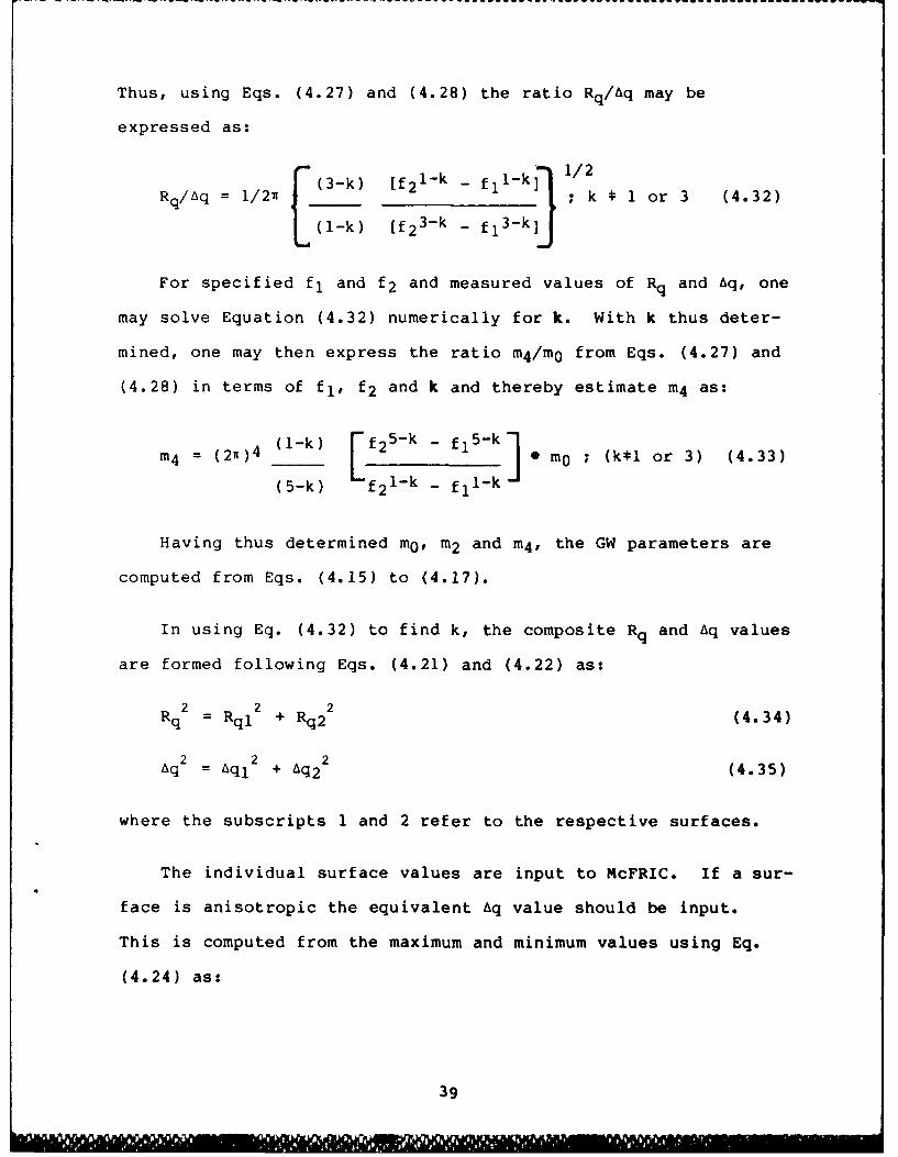
Thus, using Eqs. (4.27) and (4.28) the ratio Rq/Aq may be
expressed as:
F 3k_ ~ - 1/2
Rq/Aq = 1/2 _3 L2 - ; k * 1 or 3 (4.32)
(1-k) [f23-k - fl3-k]
For specified fl and f2 and measured values of Rq and aq, one
may solve Equation (4.32) numerically for k. With k thus deter-
mined, one may then express the ratio m4/m0 from Eqs. (4.27) and
(4.28) in terms of fl, f2 and k and thereby estimate m4 as:
m4 2 )( l-k) Ff25-k - fl5 -k1
N = (21)4( m0 ; (k*l or 3) (4.33)
(5-k) f2 1- k - fl l- k
Having thus determined m0, m2 and N4, the GW parameters are
computed from Eqs. (4.15) to (4.17).
In using Eq. (4.32) to find k, the composite Rq and Aq values
are formed following Eqs. (4.21) and (4.22) as:
Rq2 = Rql2 + Rq22 (4.34)
2 2 2Aq = AqI + Aq2 (4.35)
where the subscripts 1 and 2 refer to the respective surfaces.
The individual surface values are input to McFRIC. If a sur-
face is anisotropic the equivalent Aq value should be input.
This is computed from the maximum and minimum values using Eq.
(4.24) as:
39

Aqe = [(Aq)MAx * (Aq)MINI/ 2 (4.36)
4.5 Expected Values of Traction Force Components
and Torque at Asperities
The contact ellipse dimensions are assumed to have their dry
contact values. The fluid pressure at a general position within
the contact ellipse is assumed to be reduced by asperity loading
but to remain proportional to the dry contact pressure:
0(x,y) = 80 [l-(x/a)2 - (y/b)2 ]]2 (4.37)
* where 6 is a constant of proportionality.
The value of 0 is determined by requiring that the sum of the
load supported by elastic asperity deformation (TOTF) and the
fluid pressure equilibrate the applied load P, i.e.
(2/3 6o o + TOTF)71ab = P (4.38)
so that
0 = 1.5 [P/rab - TOTF]/00 (4.39)
The solution requires, of course, that P > TOTF wab and may be[ invalid for thin films and light loads.
6For lubricant films that are thick relative to the surface
roughness TOTF = 0 and 8 = 1.0.
40
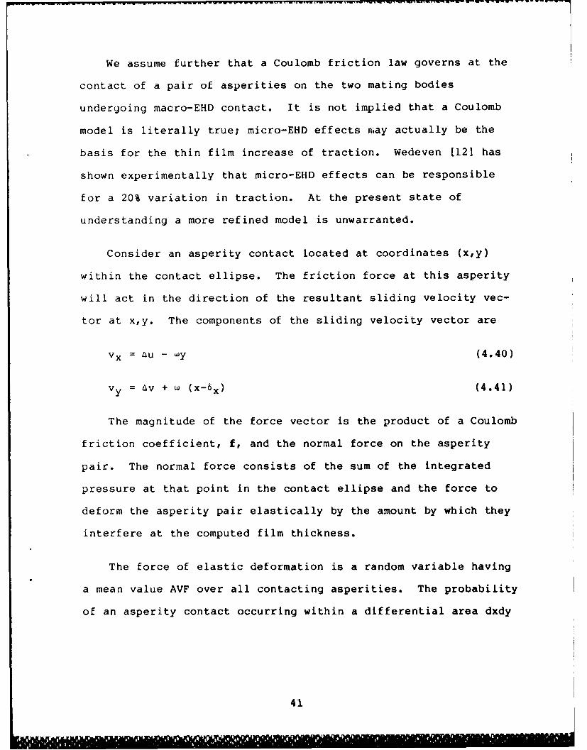
We assume further that a Coulomb friction law governs at the
contact of a pair of asperities on the two mating bodies
undergoing macro-EHD contact. It is not implied that a Coulomb
model is literally true; micro-EHD effects may actually be the
basis for the thin film increase of traction. Wedeven [121 has
shown experimentally that micro-EHD effects can be responsible
for a 20% variation in traction. At the present state of
understanding a more refined model is unwarranted.
Consider an asperity contact located at coordinates (x,y)
within the contact ellipse. The friction force at this asperity
will act in the direction of the resultant sliding velocity vec-
tor at x,y. The components of the sliding velocity vector are
vx = AU - Wy (4.40)
V y = Av + W (x-6x ) (4.41)
The magnitude of the force vector is the product of a Coulomb
friction coefficient, f, and the normal force on the asperity
pair. The normal force consists of the sum of the integrated
pressure at that point in the contact ellipse and the force to
deform the asperity pair elastically by the amount by which they
interfere at the computed film thickness.
The force of elastic deformation is a random variable having
a mean value AVF over all contacting asperities. The probability
of an asperity contact occurring within a differential area dxdy
41
+ [ "" + I" + r + ' MM

within the macrocontact ellipse, is, to a first approximation,
independent of coordinate position.
This probability is the product of the number of contacts per
unit area ZNCON and the differential area dxdy, i.e.
PROB [Contact in dxdy] = (ZNCON) dxdy (4.42)
The expected normal force due to elastic deformation at (x,y)
is thus
E(N) = (AVF * ZNCON) dxdy (4.43)
The expected friction force at position (x,y) is thus
E(F(x,y)) = f [AVF 0 ZNCON + TOTA * Oa (x,y)] dxdy (4.44)
where o(x,y) is the Hertzian pressure distribution. 0 is the
fluid pressure reduction factor and TOTA is the total asperity
area per unit nominal area.
The x component of the total expected friction force is found
by integrating the x projection of E(F(x,y)) over the contact
ellipse, i.e.
E(Fx) = fff [AVFOZNCON + TOTA 0 0o(x,y)]fvx/(v 2 x + vy 2 ) ldxdy
(4.45)
The y component is similarly defined but with Vy replacing vx
in the numerator of the integrand.
42
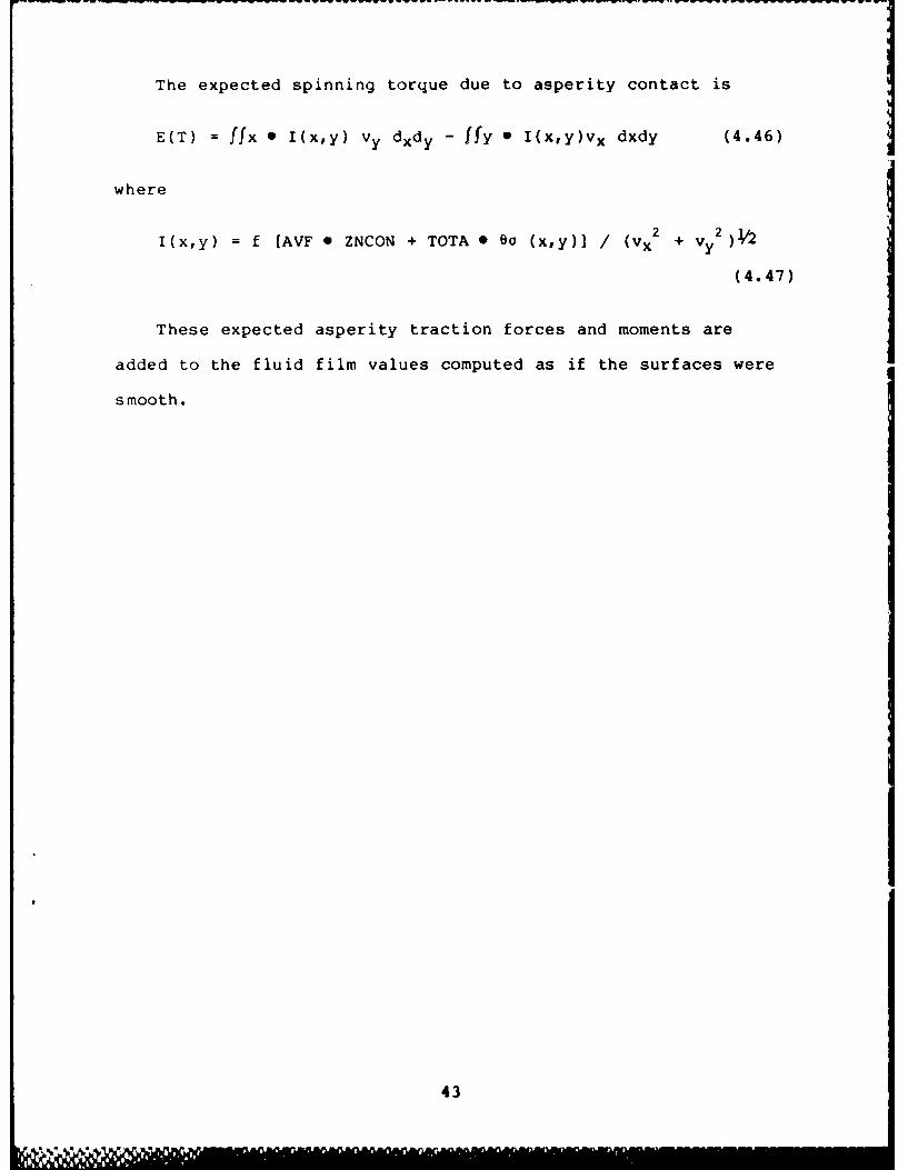
The expected spinning torque due to asperity contact is
E(T) = ffx 0 I(x,y) Vy dxdy - fly 0 I(x,y)v x dxdy (4.46)
where
I(x,y) = f [AVF 0 ZNCON + TOTA 6 ao (x,y)] / (vx 2 + vy 2
(4.47)
These expected asperity traction forces and moments are
added to the fluid film values computed as if the surfaces were
smooth.
43
5.0 RHEOLOGICAL MODEL FOR FLUID TRACTION
5.1 One Dimensional Maxwell Model
A survey of the literature on traction in concentrated con-
tacts was made in conjunction with this project, and a summary
account is given in the Interim Report [13]. A pivotal paper in
.5 the traction literature, noted therein, is that of Johnson and
Roberts [141, in which it was ingeniously established experimen-
tally that a fluid in a concentrated contact can deform elasti-
cally at sufficiently high pressures and rolling velocities. The
key to this demonstration is the fact that a lateral force deve-
lops in the presence of spin with an elastic fluid, but not if
the fluid deforms viscously. This lateral force was shown by
Gentle and Boness [151 to be essential for correctly predicting
the steady state ball rotational axis in angular contact ball
bearings.
To account for the viscoelastic response, Johnson and Roberts
proposed that the lubricant be regarded as a Maxwell fluid in
which, on the application of a shear rate y, the fluid shear
stress T varies with time t in accordance with the differential
equation:
(1/G) dT/dt + /n = (5.1)
Essentially, this model regards the strain rate t as con-
sisting of two components: an elastic strain rate ie given by
44i4
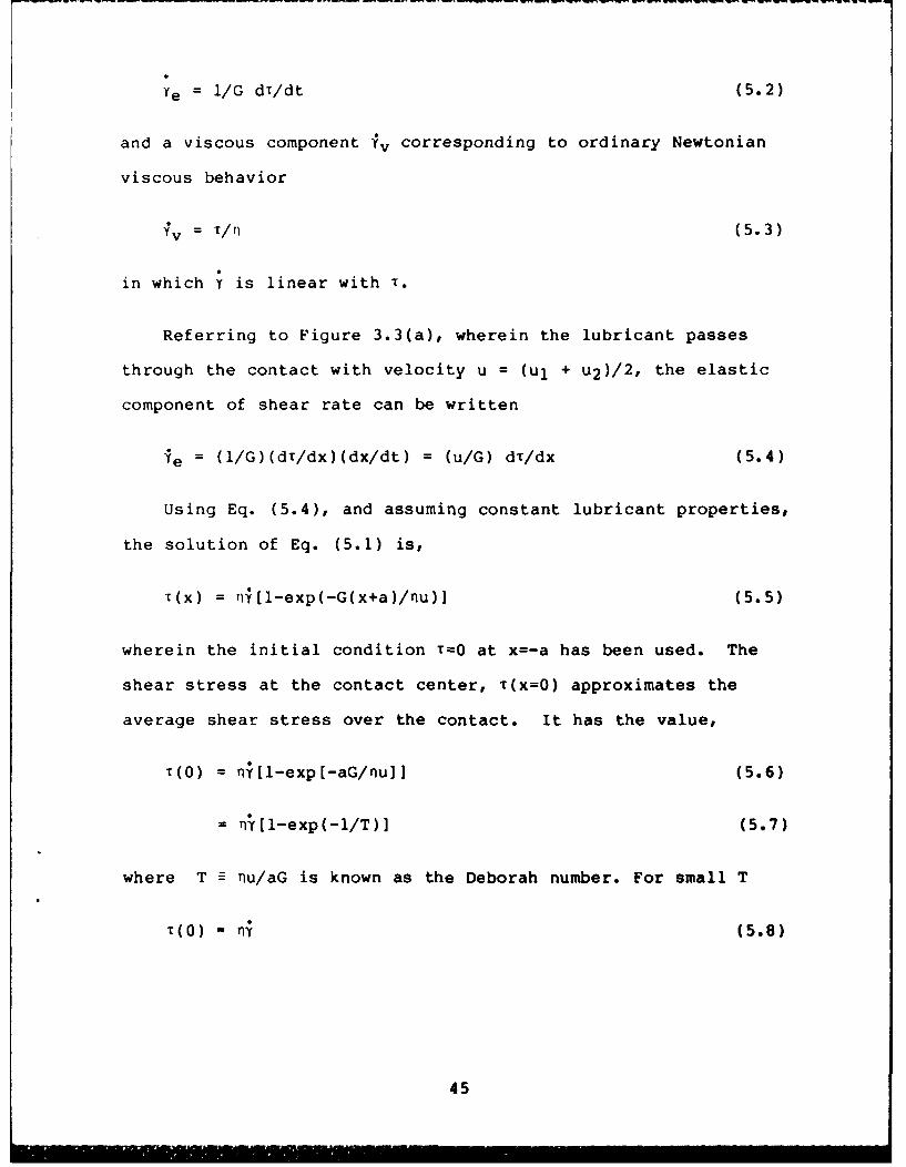
;e = 1/G dT/dt (5.2)
and a viscous component 1v corresponding to ordinary Newtonian
viscous behavior
= T/1) (5.3)
in which Y is linear with T.
Referring to Figure 3.3(a), wherein the lubricant passes
through the contact with velocity u = (uI + u2 )/2, the elastic
component of shear rate can be written
le = (I/G)(dT/dx)(dx/dt) = (u/G) dT/dx (5.4)
Using Eq. (5.4), and assuming constant lubricant properties,
the solution of Eq. (5.1) is,
1(x) = ,i[l-exp(-G(x+a)/nu)] (5.5)
wherein the initial condition T=O at x=-a has been used. The
shear stress at the contact center, x(x=O) approximates the
average shear stress over the contact. It has the value,
T(O) = ni[l-exp[-aG/nu]] (5.6)
= n [1l-exp(-1/T)] (5.7)
where T E nu/aG is known as the Deborah number. For small T
-(0) - n (5.8)
45
- -.. . . " -- - - - - -l '- - . .
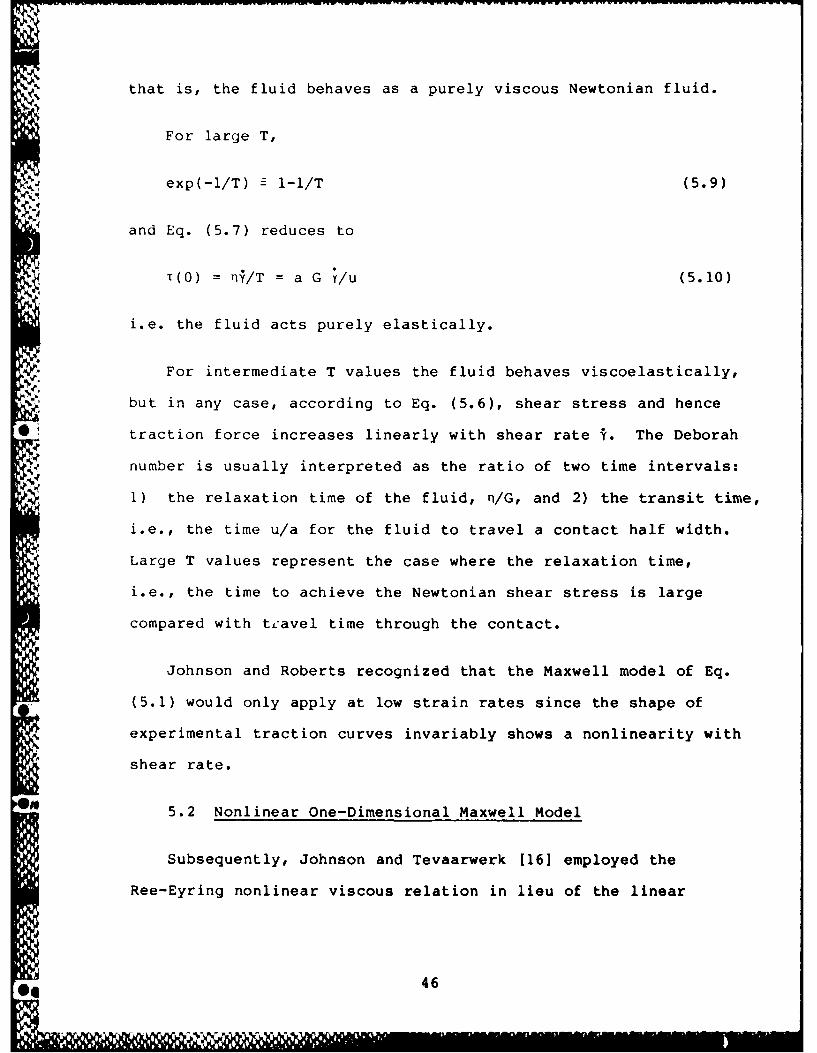
that is, the fluid behaves as a purely viscous Newtonian fluid.
For large T,
exp(-l/T) E 1-1/T (5.9)
and Eq. (5.7) reduces to
T(0) = nj/T = a G ;/u (5.10)
i.e. the fluid acts purely elastically.
For intermediate T values the fluid behaves viscoelastically,
*but in any case, according to Eq. (5.6), shear stress and hence
*! traction force increases linearly with shear rate %. The Deborah
number is usually interpreted as the ratio of two time intervals:
1) the relaxation time of the fluid, n/G, and 2) the transit time,
i.e., the time u/a for the fluid to travel a contact half width.
Large T values represent the case where the relaxation time,
i.e., the time to achieve the Newtonian shear stress is large
compared with tzavel time through the contact.
Johnson and Roberts recognized that the Maxwell model of Eq.
(5.1) would only apply at low strain rates since the shape of
experimental traction curves invariably shows a nonlinearity with
shear rate.
5.2 Nonlinear One-Dimensional Maxwell Model
Subsequently, Johnson and Tevaarwerk [16] employed the
Ree-Eyring nonlinear viscous relation in lieu of the linear
46
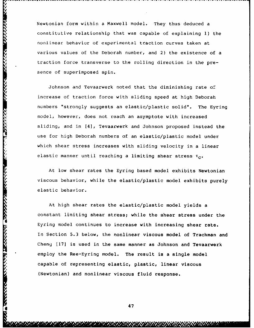
Newtonian form within a Maxwell model. They thus deduced a
constitutive relationship that was capable of explaining 1) the
nonlinear behavior of experimental traction curves taken at
various values of the Deborah number, and 2) the existence of a
traction force transverse to the rolling direction in the pre-
sence of superimposed spin.
Johnson and Tevaarwerk noted that the diminishing rate of
increase of traction force with sliding speed at high Deborah
numbers "strongly suggests an elastic/plastic solid". The Eyring
model, however, does not reach an asymptote with increased
sliding, and in [4], Tevaarwerk and Johnson proposed instead the
use for high Deborah numbers of an elastic/plastic model under
which shear stress increases with sliding velocity in a linear
elastic manner until reaching a limiting shear stress Tc.
At low shear rates the Eyring based model exhibits Newtonian
viscous behavior, while the elastic/plastic model exhibits purely
elastic behavior.
At high shear rates the elastic/plastic model yields a
constant limiting shear stress; while the shear stress under the
Eyring model continues to increase with increasing shear rate.
In Section 5.3 below, the nonlinear viscous model of Trachman and
Cheng [17] is used in the same manner as Johnson and Tevaarwerk
employ the Ree-Eyring model. The result is a single model
capable of representing elastic, plastic, linear viscous
(Newtonian) and nonlinear viscous fluid response.
6 47
5.3 The Trachman-Cheng Nonlinear Viscous Model
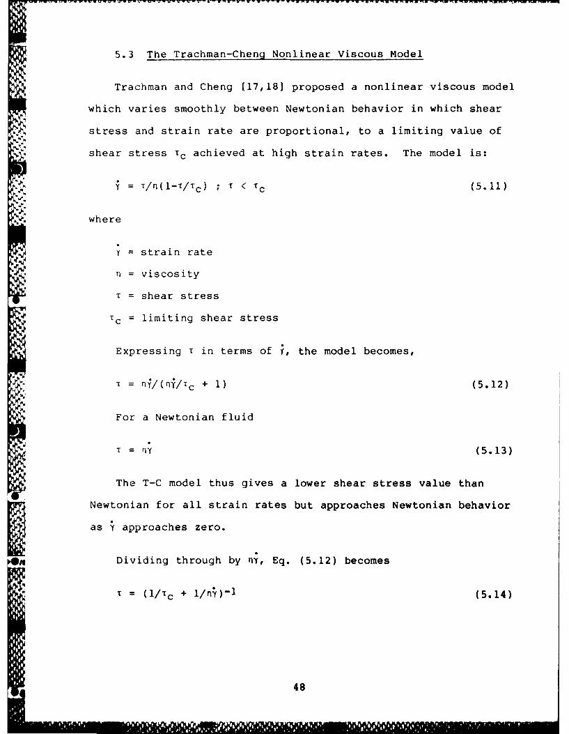
Trachman and Cheng [17,181 proposed a nonlinear viscous model
which varies smoothly between Newtonian behavior in which shear
stress and strain rate are proportional, to a limiting value of
shear stress Tc achieved at high strain rates. The model is:
T/n(l-T/tc) ; T < Tc (5.11)
where
; = strain rate
n = viscosity
T = shear stress
c = limiting shear stress
Expressing T in terms of , the model becomes,
,. -., = n;/(r(n/Tc + 1) (5.12)
For a Newtonian fluid
-= ry (5. 13)
The T-C model thus gives a lower shear stress value than
Newtonian for all strain rates but approaches Newtonian behavior
as ' approaches zero.
'U Dividing through by n;, Eq. (5.12) becomes
T = (i/Tc + l/ny)1 (5.14)
48

In this form it is seen that for Y large, T approaches Tc.
Thus, of itself, the T-C model accommodates Newtonian behavior
at low strain rates and plastic behavior at large strain rates.
For an elastic fluid as we have seen
= (U/G) dT/dx (5.15)
5.4 The Nonlinear One-Dimensional Maxwell Model
Using the Trachman-Cheng Viscous Component
Following Tevaarwerk and Johnson, we express the total strain
rate y as the sum of an elastic strain rate E and a (nonlinear)
viscous strain rate YV:
= iE + V (5.16)
Using Eq. (5.15) for TE and the T-C model, Eq. (5.11), for iV
leads after rearrangement to the following differential equation
for T
dt/dx = G'/u - GTc/Un * T/(TC-T) (5.17)
5.5 Application to a Line Contact
In order to evaluate the model implications, a line contact
(or a strip across an elliptical contact) of width 2a and with an
x coordinate established at the contact center is now considered
49
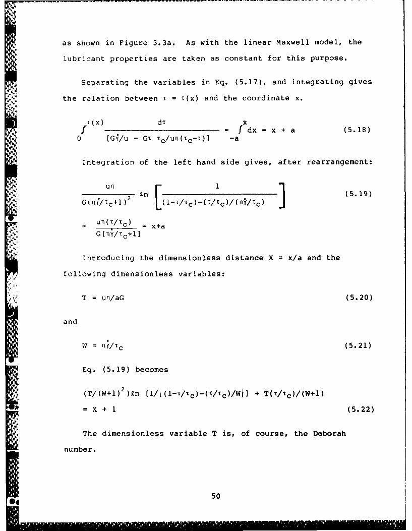
as shown in Figure 3.3a. As with the linear Maxwell model, the
lubricant properties are taken as constant for this purpose.
Separating the variables in Eq. (5.17), and integrating gives
the relation between T = T(x) and the coordinate x.
c (x) dT x
f = f dx = x + a (5.18)0 [Gi/u - GT Tc/Un(TC-T)] -a
Integration of the left hand side gives, after rearrangement:
un 2 n 1(5.19)
G ( rrY'/t c+ 1 ) ( l1-/TC) ( /Tc)/( n'/Tc J+ un (T/tc) = x+a
G [nY/T c+l]
Introducing the dimensionless distance X = x/a and the
following dimensionless variables:
T = un/aG (5.20)
and
W = ,l;/T c (5.21)
Eq. (5.19) becomes
(T/(W+l) 2 )n [l/t (1-r/TC)-(T/Tc)/Wj] + T(T/Tc)/(W+l)
= X + 1 (5.22)
The dimensionless variable T is, of course, the Deborah
number.
S 50
. r " ... "... ,- - ,: .t,, , F ,., F - ' '" ".' F -A N ..... '

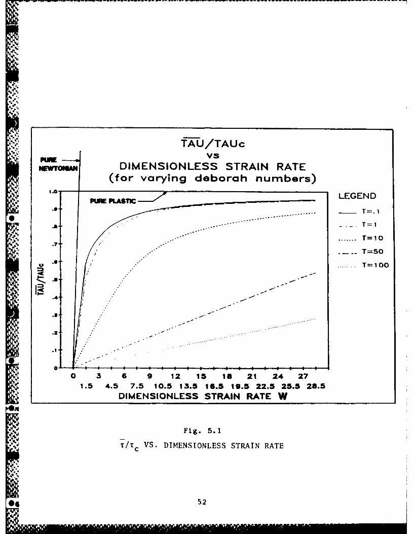
Eq. (5.22) has been solved to yield the dimensionless shear
stress i/rc as a function of dimensionless shear rate W for
various values of T and coordinate position X. Integrating
across the contact, i.e. with respect to X, yields the average
value t/rc as a function of W with T as a parameter. Figures 5.1
and 5.2 show T/Tc as a function of W and of W/T, respectively. It
is of interest to show how certain limiting forms, viz. the
Newtonian viscous, the pure elastic and the pure plastic models
appear on these grids.
Newtonian Viscous Model
For a Newtonian purely viscous model,
T = rn¥ (5.23)
so that
T/Tc = nY/Tc = W (5.24)
represents a Newtonian viscous model. Since under this model
E/Tc does not depend on x, the average value, T/Tc is also aqual
to W. The value of T/Tc for a Newtonian viscous model thus plots
against W as a line of unit slope. This Newtonian limit is shown
in Figure 5.1. On a plot of t/Tc against W/T, a Newtonian viscous
model will appear as a straight line with a slope equal to the
Deborah number. The curve for T = 0.001 in Figure 5.2 is suf-
ficiently straight to suggest nearly Newtonian viscous behavior.
51
TAU/TAUcRM vs
NEWTONMDIMENSIONLESS STRAIN RATE(for varying deborah numbers)
p. -qSI LEGEND
.6 T=.
T=5
.. ............................................ . . .............. T O
. . . . .. . . . . . . . . . ......... . .
0 3 6 9 12 1s Is 21 24 271.5 4.5 7.5 10.5 13.5 16.5 19.5 22.5 25.5 283.5
DIMENSIONLESS STRAIN RATE W
Fig. 5.1
l'n cVS. DIMENSIONLESS STRAIN RATE
04 52
TAU/TAUcvs
PM DIMENSIONLESS STRAIN RATE W/TBAS~iC(for varying deborah numbers)
7- LEGEND.0PURE PLASTIC-'.... T.0
T=.001....T=.05
ji T=l..... T-10
.... ... ... -
o 20 40 60 80 100 120 140 160 16010 30 50 70 90 110 130 130 170 190
DIMENSIONLESS STRAIN RATE W/T
Fig. 5.2
c/ VS. DIMENSIONLESS STRAIN RATE W/T
53

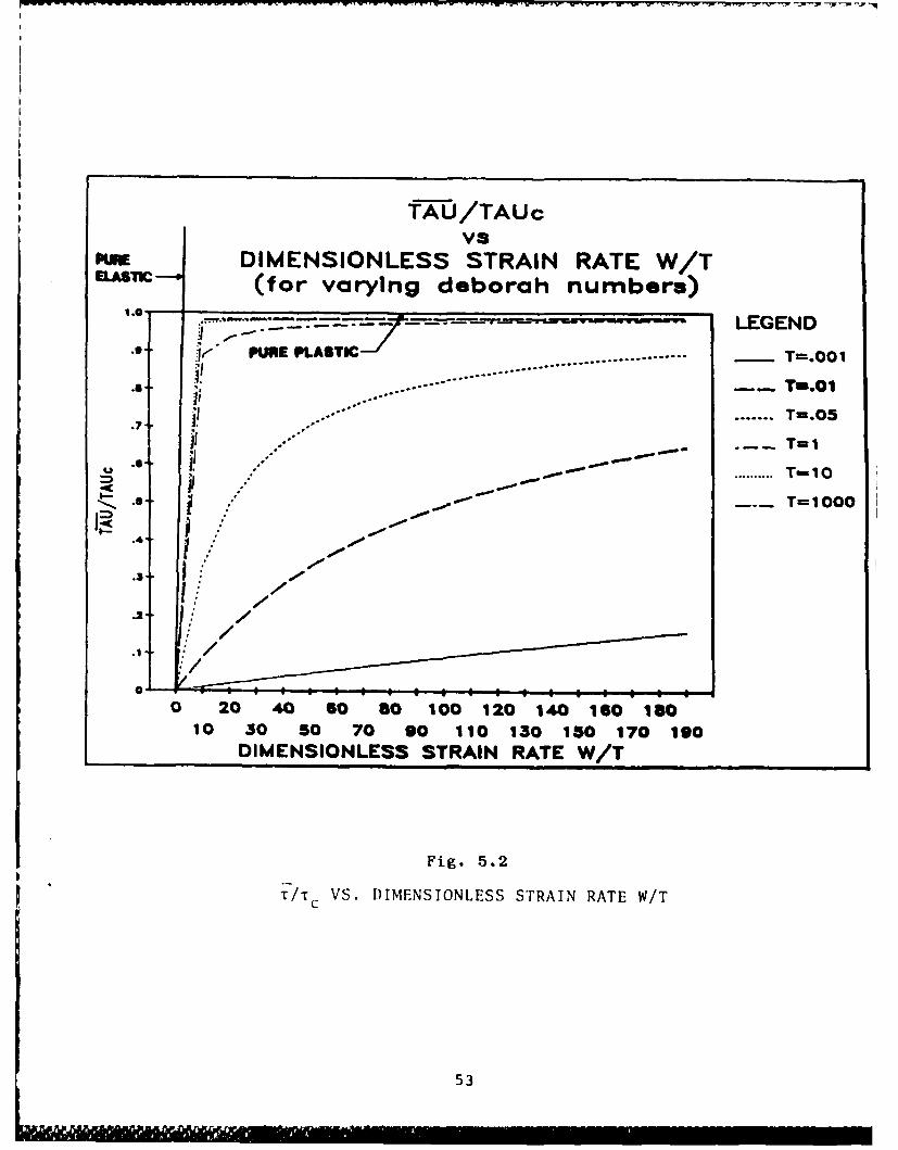
Purely Plastic Model
A purely plastic model is represented by
or i/Ic = 1.0 = T/rc (5.25)
This line is shown on Figures 5.1 and 5.2.
Purely Elastic Model
For a purely elastic model one may integrate Eq. (5.14) to give:
I G';aX + c/u (5.26)
where c is a constant of integration.
Using the initial condition T = 0 at X = -1, gives
T/Tc = Gya/u'c (X+I) = (W/T)(X+l) (5.27)
Since this expression is linear in X, T/Tc is equal to T/Ic at
the average value of X, i.e. at X = 0.
Thus,
T/Ic = W/T (5.28)
In a plot of T/Tc against W/T, the pure elastic model will
thus have unit slope. This pure elastic limit line is shown
drawn on Figure 5.2.
54
In a plot against W, the pure elastic model is a straight
line of slope l/T. The curve shown in Figure 5.1 for T = 50
appears straight to within graphical accuracy and thus represents
primarily elastic behavior.
Bidimensional Constitutive Law
Following Johnson and Tevaarwerk [16], the lubricant film in
the contact in which shear stresses are developed, is assumed to
be uniform and thin.
The flow due to the pressure gradient in the EHD contact is
ignored as negligible over the high pressure region, with the
consequence (from the momentum equation) that the shear stress in
the x and y directions does not vary across the thickness of the
film. In these circumstances the bidirectional version of the
constitutive relation that was adopted for the one dimensional
case in Section 5.0, becomes the coupled system of differential
equations:
Udr + x e (5.29)
Gdx Te n(l-Te/Tc)
+ e te = /r y (5.30)Gdx Te n(l-Te/Tc )
where rx and Ty are the orthogonal components of the interfacial
shear stress. Te, the equivalent shear stress, is defined as:
55
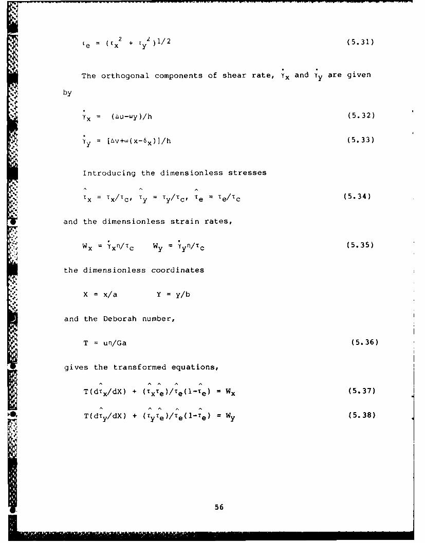
x= ( 2 + 1 2 )1/2 (5.31)
The orthogonal components of shear rate, ;x and ;y are given
by
;x = (Lu-wy)/h (5.32)
y = [Lv+u(x-6x)I/h (5.33)
Introducing the dimensionless stresses
= x Tx/T c Ty = ty/tc' re = te/Ic (5.34)
and the dimensionless strain rates,
Ywx =xn/Tc Wy = ;y n/TC (5.35)
the dimensionless coordinates
X = x/a Y = y/b
and the Deborah number,
T = un/Ga (5.36)
gives the transformed equations,
T(dTx/dX) + (TxTe)/Te(l-Te) = Wx (5.37)
0. T(dTy/dX) + (TyTe)/Te(l-Te) = Wy (5.38)
56
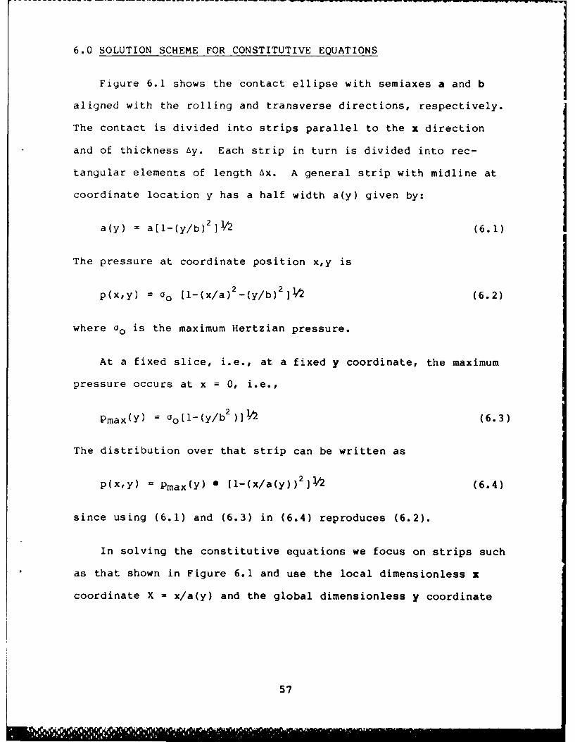
6.0 SOLUTION SCHEME FOR CONSTITUTIVE EQUATIONS
Figure 6.1 shows the contact ellipse with semiaxes a and b
aligned with the rolling and transverse directions, respectively.
The contact is divided into strips parallel to the x direction
and of thickness Ay. Each strip in turn is divided into rec-
tangular elements of length Ax. A general strip with midline at
coordinate location y has a half width a(y) given by:
a(y) = a[l-(y/b)2 ] /2 (6.1)
The pressure at coordinate position x,y is
p(x,y) = Go [l-(x/a) 2 -(y/b) 2 ] 2 (6.2)
where 00 is the maximum Hertzian pressure.
At a fixed slice, i.e., at a fixed y coordinate, the maximum
pressure occurs at x = 0, i.e.,
Pmax(Y) = o0 [l-(y/b2 )]2 (6.3)
The distribution over that strip can be written as
p(x,y) = Pmax(Y) * [l-(x/a(y))2 ]2 (6.4)
since using (6.1) and (6.3) in (6.4) reproduces (6.2).
In solving the constitutive equations we focus on strips such
as that shown in Figure 6.1 and use the local dimensionless x
coordinate X = x/a(y) and the global dimensionless y coordinate
57
! I "" .. ....d

Vy
XI1~ y
-I-.mA(y
Fig. 6.1 CONTACT ELLIPSE COORDINATE SYSTEM
58
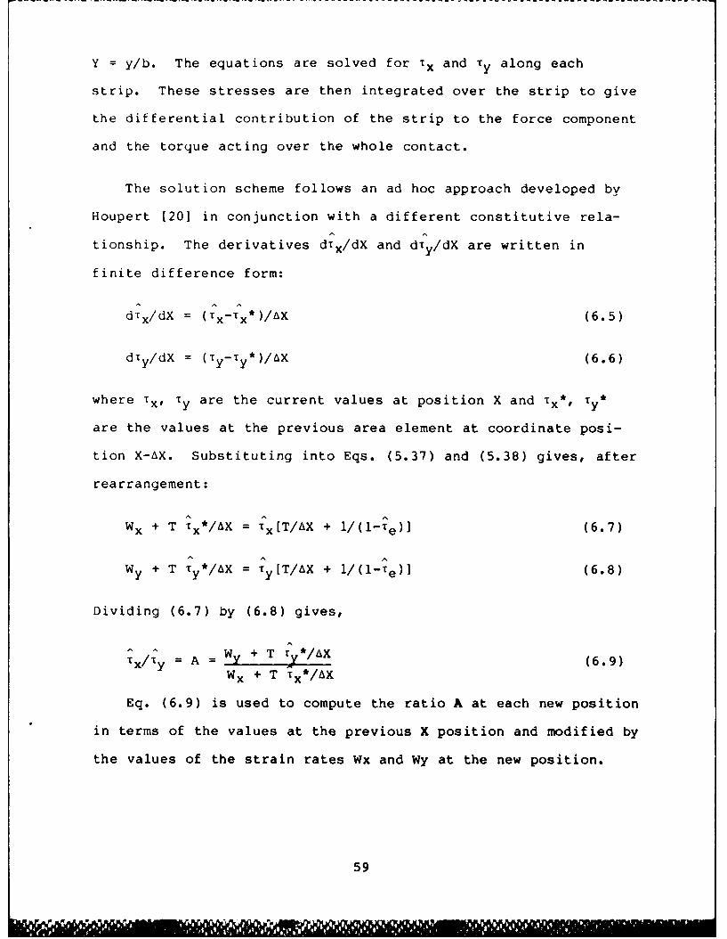
Y = y/b. The equations are solved for t x and ty along each
strip. These stresses are then integrated over the strip to give
the differential contribution of the strip to the force component
and the torque acting over the whole contact.
The solution scheme follows an ad hoc approach developed by
Houpert [201 in conjunction with a different constitutive rela-
tionship. The derivatives drx/dX and dry/dX are written in
finite difference form:
dtx/dX = (Tx-rx*)/AX (6.5)
dTy/dX = (Ty-iy*)/AX (6.6)
where x,, Ty are the current values at position X and TX* Ty *
are the values at the previous area element at coordinate posi-
tion X-AX. Substituting into Eqs. (5.37) and (5.38) gives, after
rearrangement:
Wx + T tX*/AX = tx[T/AX + 1/( 1 -*e)] (6.7)
Wy + T Ty*/AX = Ty[T/AX + i/(l-Te)] (6.8)
Dividing (6.7) by (6.8) gives,
Ax/Sy = A = WY + T r*/AX (6.9)
Wx + T T x*/AX
Eq. (6.9) is used to compute the ratio A at each new position
in terms of the values at the previous X position and modified by
the values of the strain rates Wx and Wy at the new position.
59
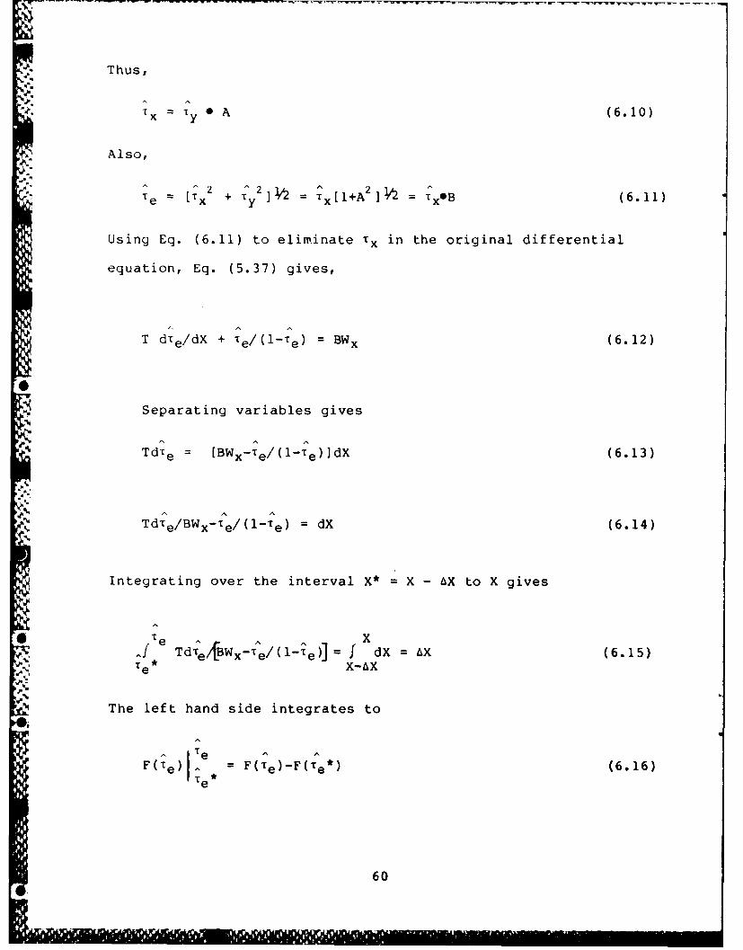
Thus,
Tx T* 0A (6. 10)
Also,
[Tx2 + ~' ~ TxI~l+A 2 x = B (6.11)
Using Eq. (6.11) to eliminate Tx in the original differential
equation, Eq. (5.37) gives,
T dle/dX + Te/ (1T e) = BWx (6. 12)
Separating variables gives
Td-re = [BWX-T e/ (1T e)IdX (6.13)
a.TdT e/BWx-Te/ (1-Te) = dX (.4
Integrating over the interval X* X -AX to X gives
AT TdeB xe(Te f dX =AX (6.15)T e * XX
The left hand side integrates to
F(T e)I^ = F(T e)-F(T e*) (6.16)ITe
60
whe re
F(te) = T/(BWx+I) 2 £n [1-(1+I/BWx)Te] + TeT/(BWx+1) (6.17)
Given ie* at the abscissa value X*, the next successive value
is found by numerically solving:
F(le) - F(Te*) = AX (6.18)
A golden section search technique is used to implement the solu-
tion. Having thus found Te, Te is found as
're T C*c'e (6.19)
T . and 'y are then computed as
Ex = Te/B (6.20)
T y = Tx/A (6.21)
The solution scheme starts with Te=O at the inlet end of the
strip and bootstraps across the strip length solving for the
stress on the next successive element located at the distance AX
further down the strip. Inasmuch as the lubricant properties
depend on the local pressure and temperature at each successive
location, they are adjusted to the local conditions of each ele-
ment using properties relationships discussed further below.
61

The actual stresses Tx and Ty are obtained by multiplying T x
and ty by the locally variable value of Tc. The differential
torque contribution at location x,y is
5 DT(x,y) = T * y - y (X-6x) (6.22)
T xy and dT(x,y) are integrated over the strip at position y to
yield the differential force components dFx(y), dFy(y) and the
differential torque contribution of the strip dT(y).
a(y)dFx(y) = T txdx (6.23)
" -a(y)
a(y)dFy(y) = J Ty dx (6.24)
-a(y)
a(y)dT(y) = 2 dT(x,y)dx (6.25)
-a(y)
Once these quantities are evaluated for each strip of the contact
ellipse they are integrated across the strips to give the total
fluid force and torque components:
bFx = j dFx(y)dy (6.26)
-b
bFy = J dFy(y)dy (6.27)
-b
bT = J dT(y)dy (6.28)
-b
62
The combined fluid and asperity friction forces are obtained
N by summing the fluid force components and spinning torque from
Eqs. (6.26)-(6.28) and the corresponding expected coulomb fric-
tion values from Eqs. (4.45) and (4.46). Denote these sums Fx ,
Fy and T.
The combined frictional power loss (EL) may then be computed
as
EL = Fx 0 Au + Fy 0 Av + T 0 w (6.29)
For some applications, most notably traction drives, the
power transmitted (ET) through the contact is of critical impor-
tance. This is
ET = Fx 0 u (6.30)
The loss factor (LF) is computed as the ratio of the power
loss to the power transmitted, i.e.
L. = EL/ET (6.31)
.6
I
66
7.0 HEAT GENERATION AND THERMAL ANALYSIS
7.1 Heat Generation
The heat generated per unit volume is computed point-by-point
along each strip in the contact area. The total heat input per
unit volume, Q, is the sum of the contribution due to shearing of
*" the fluid, Qf, and due to the coulomb friction at the asperities,
Qa.
71.1 Fluid Shear Heat
The fluid contribution is computed as the product of the
resultant shear stress
-[x 2 + y2 ] 1/2 (7.1)
and the viscous component of the shear rate v" The recoverable
elastic shear is thus not included in computing fluid heat
generation. Using Eq. (5.11) gives
v= Te/n(l1Te/Tc) (7.2)
4so that
Qf =Te * 1v (7.3)
Since Yv must not exceed Y, a numerical check is made. If
v>;, Qf is computed as
64
0n
S . - -
Qf = Te (7.4)
7.1.2 Heat Generated at Asperities
As noted in Section 4.0, the quantity TOTF computed using the
Greenwood-Williamson microcontact model is the asperity load per
unit area of apparent contact. With a coulomb friction coef-
ficient P, the traction force per unit area is PTOTF.
Multiplying by the resultant sliding velocity and dividing by
film thickness h gives the asperity generated heat per unit
apparent volume, i.e.
= PTOTF[vx2 + vy 2i/2/h = POTOTFO (7.5)
where vx and vy are the sliding velocity components:
vx = av-wy (4.40)
vy = Av+w(x-6x) (4.41)
7.2 Thermal Analysis
7.2.1 Temperature Distribution in Solid and Film
It is assumed that heat generated within the film along a
strip in the x direction as shown in Fig. 6.1 is conducted to the
two surfaces and carried by convection in the direction of
rolling. Conduction in the y direction is neglected as negli-
gible. This permits the independent analysis of the strips which
comprise the total contact.
65

It is also assumed that both the solids bounding the lubri-
cant film have the same thermal properties and the same ambient
temperature Uo. The maximum film temperature thus occurs on and
is symmetrical about the center plane. The common temperature of
the bounding solid 0s(x) varies with coordinate x and may be
expressed as the sum of the ambient temperature and the increase
'- £Lus(x) caused by heating in the contact. The maximum film tem-
.* perature dc, in turn is expressed as the sum of the solid tem-
perature at the given coordinate position and the increase A c(x)
of the center film temperature over the solid temperature, i.e.:
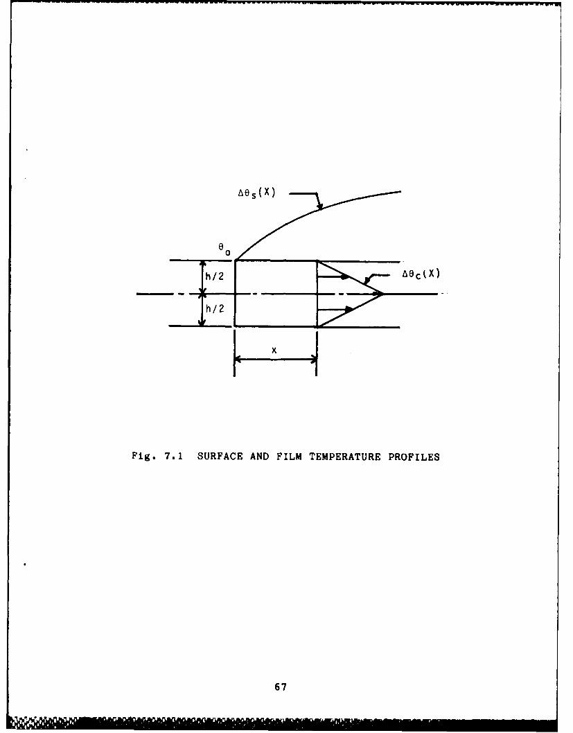
Uc(x) = Us(x) + Lc(x) (7.6)
, Uc(x) = o + AUs(x) + Aoc(x) (7.7)
Fig. 7.1 shows the temperature profile of the solids as a
function of coordinate position x and the temperature profile
across the film at a specific x position. Following Houpert
[20,211 we assume that the temperature profile across the film
has a nearly triangular shape. With this assumption, Jaeger's
equation [221 for computing AOs(x) becomes
x
.As(x) = [7,Pmmkmp]-i/ 2 J 2kAOc/h x-4]I/ 2 dW (7.8)I -a(y)
wherePe
= density
c specific heat
6604Tf"'', ' ' ', '1 " "
Aees(x)
6 -0
Fig. 7.1 SURFACE AND FILM TEMPERATURE PROFILES
67
k = thermal conductivity
h = film thickness
a(y) = half width of contact zone at coordinate position y
The subscript 'W' indicates that the property is that of the
'p solid.
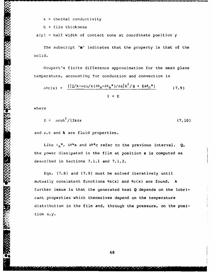
Houpert's finite difference approximation for the mean plane
temperature, accounting for conduction and convection is
abc(x) = [{Q/k-pcu/k (As-_AS*)/Axjh2/8 + EAc* (7.9)
1 + E
where
E pcuh 2 /12kAx (7.10)
and p,c and k are fluid properties.
Like lx*, Ab*S and Ab*c refer to the previous interval. 0,
the power dissipated in the film at position x is computed as
described in Sections 7.1.1 and 7.1.2.
Eqs. (7.8) and (7.9) must be solved iteratively until
mutually consistent functions bs(x) and Oc(x) are found. A
further issue is that the generated heat Q depends on the lubri-
cant properties which themselves depend on the temperature
distribution in the film and, through the pressure, on the posi-
tion x,y.
68
7.2.2 Temperature and Pressure Dependence of Lubricant
Properties
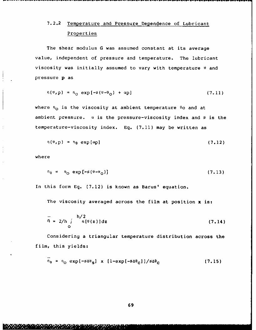
The shear modulus G was assumed constant at its average
value, independent of pressure and temperature. The lubricant
viscosity was initially assumed to vary with temperature 6 and
pressure p as
n(v,p) = no exp[-13(U-6 0 ) + ap] (7.11)
where no is the viscosity at ambient temperature eo and at
ambient pressure. a is the pressure-viscosity index and 0 is the
temperature-viscosity index. Eq. (7.11) may be written as
n(b,p) = no exp[Ap] (7.12)
where
n= no exp[- (-uo)] (7.13)
In this form Eq. (7.12) is known as Barus' equation.
The viscosity averaged across the film at position x is:
- h/2nl = 2/h J n[ (z)Idz (7.14)
0
Considering a triangular temperature distribution across the
film, this yields:
no = no exp[-tAts] x (l-exp(- Oc]1/OAOc (7.15)
69

The critical shear stress was taken to be proportional to
pressure following Tevaarwerk and Johnson [4] and, following
Lingard [26], to be inversely proportional to the absolute tern-
+" perature of the lubricant. This may be expressed as:
Tc = .p/To (7.16)
where E is a constant of proportionality, and To = bo+460 is the
absolute ambient temperature. At constant temperature, the
average value of Tc is
'cc -/To (7.17)
* Knowing tc at ambient temperature one may compute E as:
c/= p" To (7.18)
Letting Ts = Us+460 be the absolute temperature of the solid at
position x and Tc = Oc+460 the corresponding absolute temperature
of the center of the film, the mean value of Tc assuming a linear
temperature distribution across the film is
Tc = rco[To/(Tc-Ts)] ,n[Tc/Ts ] (7.19)
This expression was initially used within McFRIC but it was
found that the thermal effect on traction was over predicted using
this expression. Taking Tc to be a function of pressure only
41 resulted in greatly improved fits (cf. Section 10.0).
A In the numerical solution for temperature, an initial film
temperature rise A~c(x) was assumed by neglecting convection in
70
04
[e3YV..'
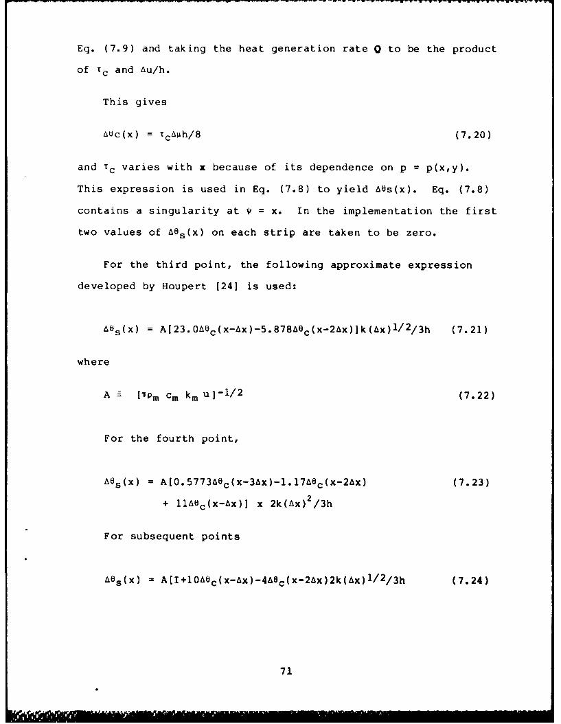
Eq. (7.9) and taking the heat generation rate Q to be the product
Of T c and Au/h.
This gives
AOC(X) = T c~iih/8 (7.20)
and T varies with x because of its dependence on p =p(x,y).
This expression is used in Eq. (7.8) to yield 6 s(x). Eq. (7.8)
contains a singularity at 4' = x. In the implementation the first
two values of A6s(x) on each strip are taken to be zero.
For the third point, the following approximate expression
developed by Houpert [24] is used:
Abs(x) = A[23. OAec(x-Ax)-5.878Aec(x-2Ax)]k (Ax)1/ 2 /3h (7.21)
where
A [1rPm cm kmu]-1/ 2 (7.22)
For the fourth point,
Ads(x) = A[O.5773Aec(x-3Ax)-l.17h0c(x-2Ax) (7.23)
+ lltUc(x-Ax)] x 2k(Ax) 2/3h
For subsequent points
Ae~)= A[I+10Abc(x-Ax)-4A~c(x-2Ax)2k(Ax)l/ 2 /3h (7.24)
71
whe re
x-Ax -Ac(4 d (7.25)I = .jd ( . 5
-a (y) V -
is evaluated numerically using Simpson's rule.
Expressions (7.21) and (7.22) are found by integrating by
parts over the singularity. Following the computation of AUS(x)
the lubricant propertis are corrected, and the generated heat
recomputed. Eq. (7.9) is then used to recompute A~c(x), now
allowing for convection.
,J
p..
~72
8.0 PROGRAM DESCRIPTION, ORGANIZATION LOGIC FLOW AND USERS
INFORMATION
8.1 Description of Computer Program
The McFRIC program computes the components of sliding trac-
tion in the rolling direction and the transverse direction
(orthogonal to the rolling direction) as well as the spinning
torque for a general elastohydrodynamic (EHD) contact that
experiences rolling, sliding and spinning. It calculates the
power transmitted and the power lost for each kinematic con-
dition. The lubricant shear force is modelled as
viscoelastic/plastic with temperature and pressure dependent
viscosity and limiting shear stress. Asperity friction is
assumed to be Coulombic and is proportional to the asperity load
computed via the Greenwood-Williamson microcontact model.
The program solution can be isothermal or it can consider the
generation of heat due to fluid shear and asperity friction and
its conduction through the film and convection along the rolling
direction. For the thermal case, the program computes film mean
plane and surface temperature distributions and outputs their
average and maximum values over the contact.
In addition to traction related output, the program computes
the contact dimensions, pressure, deflection, film thickness,
including the effects of starvation and inlet heating, Deborah
number and a surface fatigue index.
73

8.2 Program Organization
Computer program McFRIC is organized into 9 modules and
comprises, in aggregate, a main routine, 15 subroutines and 17
function subprograms. The module names and their associated
tunction and subroutine names are listed in Table 8.1. The input
data comprises 34 elements of variable data and 17 run control
variables. These input data elements are contained in an input
file prepared and named by the user by editing a sample file
supplied with the program disk. The input data is discussed
further in Section 8.4.3 below.
8.3 Program Logic Flow
Figure 8.1 shows the overall logic flow for computer program
McFRIC. On execution, the program requests that the name of an
input data file be typed from the console. This file is then
read and echoed in the printed output. The program calculates
the contact parameters using subroutine HERTZ, the film thickness
(starved, unstarved, constriction and plateau) using subroutine
FILM and Deborah number (subroutine DEBORA). The microcontact
parameters are computed using subroutine GW and a surface fatigue
index is computed within the main program. The program enters a
loop in which the sliding velocity is varied over a user spe-
cified range.
For each value of the sliding velocity the fluid traction
forces and torque are computed through subroutine TRACT and its
74

Table 8.1 MODULES, FUNCTIONS AND SUBROUTINE NAMES FOR MCFRIC
MODULE FUNCTION SUBROUTINE
MCFRIC INTEG, SIMPS, Fl MCFRIC (MAIN)PLOT
F2, F3, F1 OUTPUT
INPOUT OUTPUTINPUTPRINT
EHD SOLN HERTZELINTFILM
GW FUNO, ERFC, FUN11 GWFUN321, FUN1, FUN32 DEBORAANORM, SPECEX, FUNCSPEC4
TRACT TRACT
STRESS FUN STRESSXSTRESS
FTINT FTINT
MAXAV MAXAV
HEAT HEAT
75
'e" P q : ': ... ..C
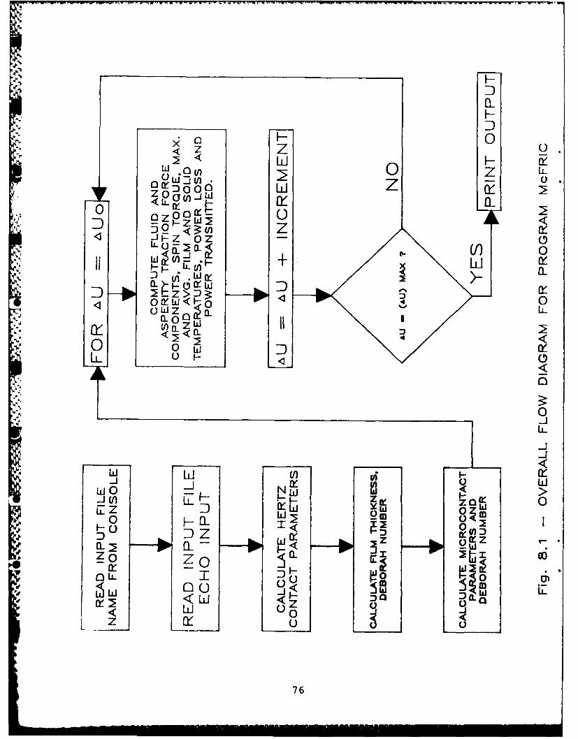
"N D0
Zi U I
0 z L0
-Z QzIV jOZ0O
<1- o z 0
LL E a-9 V 0
0 o w4LL 0_ 7-_W
______ 00
00
ILI
w 0 NW
0 F-_l 1: 0 mDZl 'D I.)
I~~~ HZ ZO
76 -- o 3
subsidiary subroutines. TRACT is discussed in more detail below.
At the completion of the traction computational loop, the
remaining program output is printed. At the user's option
printer plots may be specified in which up to 12 traction related
variables may be plotted against sliding speed.
Figure 8.2 is a detailed flow diagram for subroutine TRACT.
As noted, it computes fluid traction point-by-point over the con-
tact area, at a specified value of the sliding velocity Au. The
contact ellipse is divided into NY strips of thickness Ay =
2 b/NY. The index "I" references the individual strips. For
each strip the half width a(y) and maximum pressure p(y) are com-
puted along with the step length in the x direction Ax = 2a(y)/NX
(NX = number of elements on each strip).
The index "J" references each of the NX individual rec-
tangular elements along a strip, in the x direction. The
pressure at each element determines the viscosity n(p) and the
limiting shear Tc(p). The shear rates x and ;y are functions of
the location of each element, i.e., the x,y coordinates or,
equivalently the I and J indices. The stress components Tx and
T y and the torque contribution of the element are then found as a
function of the lubricant properties and shear rates using
subroutine STRESS which implements the solution scheme outlined
in Section 6.0. At this point, for an isothermal solution
ITHERM = 0, TRACT increments the index J, i.e., it moves to the
next adjacent element along the Ith strip.
77

INITIALIZE ARRAYS10CNIU 0COMPUTE AY CMUEF.F.T
COMPUTEUT a~y). 100 CNTINU
PMAX(y). &X
*~ Pp
COMPUTE PRESSURE CMUEOc
Fig. 8.2 -LOGIC DIAGRAM FOR SUBROUTINE TRACT
78
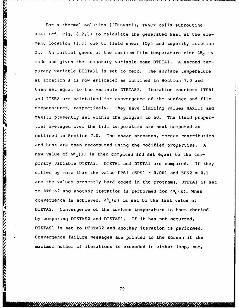
For a thermal solution (ITHERM=I), TRACT calls subroutine
HEAT (cf. Fig. 8.2.1) to calculate the generated heat at the ele-
ment location (I,J) due to fluid shear (Qf) and asperity friction
Qc" An initial guess of the maximum film temperature rise A c is
made and given the temporary variable name DTETA1. A second tem-
porary variable DTETAS1 is set to zero. The surface temperature
at location J is now estimated as outlined in Section 7.0 and
then set equal to the variable DTETAS2. Iteration counters ITERI
and ITER2 are maintained for convergence of the surface and film
* temperatures, respectively. They have limiting values MAXITI and
MAXIT2 presently set within the program to 50. The fluid proper-
ties averaged over the film temperature are next computed as
outlined in Section 7.0. The shear stresses, torque contribution
and heat are then recomputed using the modified properties. A
new value of 46c(J) is then computed and set equal to the tem-
porary variable DTETA2. DTETAI and DTETA2 are compared. If they
differ by more than the value EPSl (EPSl = 0.001 and EPS2 = 0.1
are the values presently hard coded in the program), DTETAI is set
to DTETA2 and another iteration is performed for ASc(x). When
convergence is achieved, Aec(J) is set to the last value of
DTETA2. Convergence of the surface temperature is then checked
by comparing DTETAS2 and DTETAS1. If it has not occurred,
DTETASl is set to DTETAS2 and another iteration is performed.
Convergence failure messages are printed to the screen if the
maximum number of iterations is exceeded in either loop, but,
79
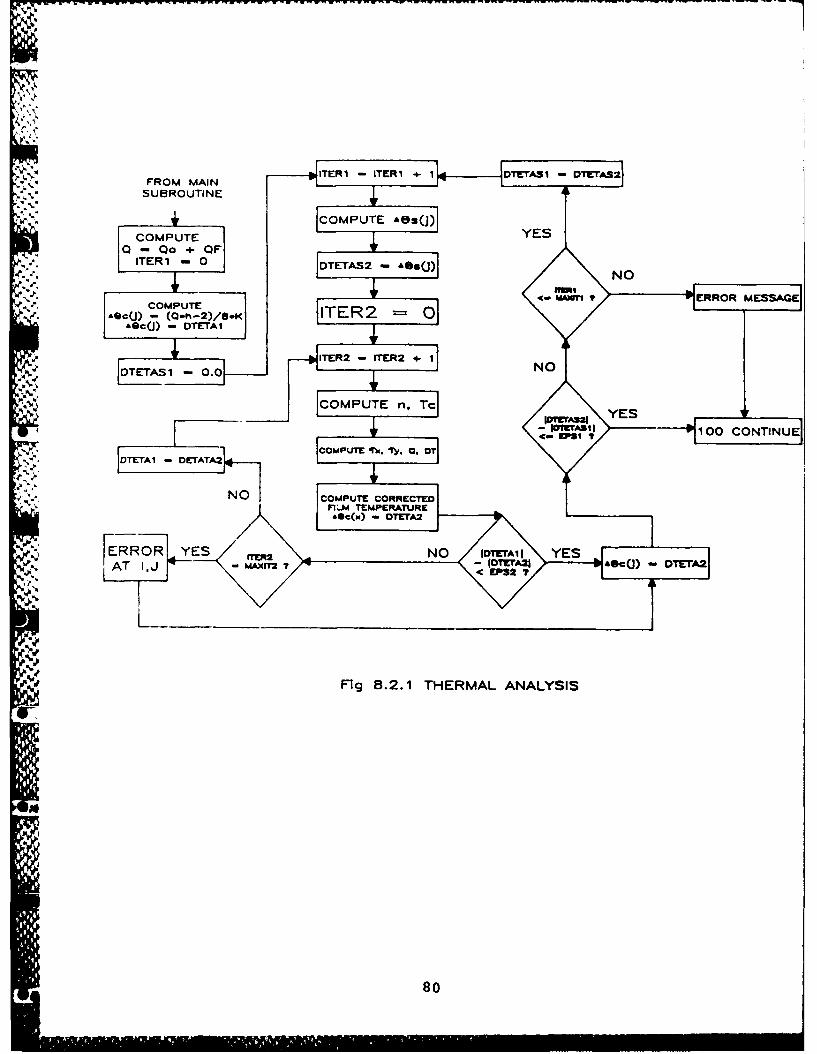
FROM MAINSUBROUTINE
COMPUTEYE0 - QO OF
ITERi 1 0 IDTETAS2 - AfO()
OMPUITE -.. rRRRMSAEAec(J) TO-h2/*
aGcQj) - TETAl 1TR
O TETASi 1 0.0 TR- E2+IN0
COMPUT YESc_ 21, E
80:
computation proceeds as indicated. (In such cases, the user must
then exercise discretion in using the results. Convergence
failure has not, however, been a problem in the test evaluations
of McFRIC discussed in Section 10.0).
When convergence is achieved for each element of a given
slice, the shear stresses and differential torque are integrated
to give the contributions DFX(I), DFY(I) and DT(I) of the slice
to the traction force components FX and FY and to the torque T.
A subroutine MAXAV is also used to find the average and maximum
solid and film temperature at the slice. When all slices are
4complete, an integration is performed over the slices to give the
• :resultant values of FX, FY and T. MAXAV is then reinvoked to
- give the overall average and maximum values of the solid and film
temperatures.
8.4 User's Information
Section 8.4 is a detailed description of how to use the
.. McFRIC program. Topics in this section include instructions for
loading and executing the program, and a discussion of the output
-data for a sample case. The information is intended to be suf-
ficient to permit a user to successfully run and interpret the
results of the McFRIC program.
8.4.1 Installing the Program
McFRIC is written in the FORTRAN language and is executable
on IBM-PC-XT or AT computers using the DOS operating system. It
81
L ' .. " ' ' ° I"
is recommended that the program be executed on a computer which
has the appropriate Math Co-processor chip (8087 or 80287)
installed.
The program is delivered on two floppy diskettes. The first
diskette (Diskette No. 1) contains the following files:
MCFRIC.EXE - Executable code for McFRIC program
MCF.BAT - Batch file for executing McFRIC program
SAMPLE.DAT - Sample problem data file
The second diskette (Diskette No. 2) contains source code
files (.FOR) for the modules making up the McFRIC program:
MCFRIC, INPOUT, EHD, GW, TRACT, STRESS, FTINT, MAXAV, and HEAT.
It is recommended for ease and speed of execution that the
program be installed on the IBM-PC hard disk. To copy the
program onto the hard disk, use the following procedure:
1. Turn on the computer and set the default drive to C:
2. Insert Diskette No. 1 into Drive A
3. Issue the command COPY A:*.*
* When the copy operation is completed, remove the floppy diskette
and store it in a safe location. If desired, Diskette No. 2 can
be copied onto the hard disk using the same procedure. However,
the files on Diskette No. 2 will only be needed if the program is
to be modified.
82
8.4.2 Executing the Program
Once the program has been copied onto the hard disk, it may
be executed as follows:
1. Set default drive to C (C>)
2. Issue the following command: MCF
The program should begin execution by displaying a heading on the
screen and prompting the user for the name of an input data file.
By typing SAMPLE.DAT, the sample case data file can be used to
verify that the program is executing properly. A listing of the
sample case data file is given as Fig. 8.3. The corresponding
program output is included as Fig. 8.4. Section 8.4.3 below con-
tains instructions for creating an input data file in the format
required by the program.
8.4.3 Creating an Input Data File
The McFRIC program has been set up to read the input data
from a standard ASCII file which can reside on the hard disk
(C: _) or on a floppy disk (A: or B: ). The recommended
technique for creating a new data file is as follows:
I. Use the DOS COPY command to copy an old data file into a
new file. For example, by issuing the command COPY
C:SAMPLE.DAT C:CASEl.DAT, a new file named CASE1.DAT
will be created on the hard disk containing the sample
case data.
83

THREE TITLE LINES DESCRIBING THE RUN:.............................................................-
TEST CASE CREATED FROM WPAFB TEST DATA FILE NIBN~gOLOAD = 140.1 LBS, ROLLING VELOCITY = 748 IN/SECAMBIENT TEMPERATURE = 183 DES. F
MATERIAL DATA:
ELASTIC MODULUS OF BODY I (Ib/in*2)[EMOD(1] .. 29.5E6ELASTIC MODULUS OF BODY I Ilb/in*E2)[EMOD2)f, .. 29.5E6PCISSON'S RATIO FOR BODY I'PRAT )] .. O. 0
POISSON'S RATIO FOR BODY I,PRAT(2f] O.O
TENSILE YIELD STRESS OF SOFTER MATERIAL (lb/infU2)[SI8MAE) ... 3.62E5
0 rOULOMB FRICTION COEFFICIENT(EF] ....... 0.06"DENSITY (Ib/in"t3)'ROM] ... 0.284?PECIFIC HEAT 19tu/lIbm-deq. F)rCp~ .... 0.11THERMAL CONDUCTIVITY (lb/sec-deg. F)IAkM] ...... 7.34
GEOMETRY AND ENVIRONMENTAL DATA:
RADIUS OF BODY I TRANSVERSE TO ROLLING DIRECTION (in)AIll] ...... 0.71RADIUS OF BODY I IN ROLLING DIRECTION (in)IR12] ...... 0.75RADIUS OF BODY I TRANSVERSE TO ROLLING DIRECTION (in)(RIIII 0.71RADIUS OF BODY II IN ROLLING DIRECTION (in)[RII21...... 0.75VELOCITY OF BODY I IN ROLLINS DIRECTION (inlsec)Ull ....... 748.18VELOCITY OF BODY 11 IN ROLLING DIRECTION fin/se )[UII] ...... 748.18TRANSVERSE DIRECTION SLIDING VELOCITY (in/sec)IDELVI ..... 0.0SPINNING VELOCITY (radians/sec)(OMEGA] .... 0.0MENISCUS DISTANCE (in)(EEXS ...... 1.0
CONTACT NORMAL LOAD (Ibs) IP] Fig. 8.3 INPUT FILE - SAMPLE.DAI140.1
AMBIENT TEMPERATURE (de. F)(TANB] ..... 193,0
* 84
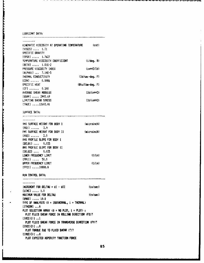
LUBRICANT DATA:
KINEMATIC VISCOSITY AT OPERATING TEMPERATURE (cst)(VISCS] .... 1.311
SPECIFIC GRAVITYISPGRJ .. 1,7627TEMPERATURE VISCOSITY COEFFICIENT 11/deq. R)[BETA) ...... 1,01E-2PRESSURE VISCOSITY INDEX tinfl2/lb)rALPHAII ... 7.14E-5THERMAL CONDUCTIVITY (Ib/sec-deg. F)(CON] ...... 0.0086SPECIFIC HEAT (Dtu/Ibe-deq. F)[CF1 ....... 0.200
*AVERAGE SHEAR MODULUS (Ib/infl2)[GEAR]..2443.69
LIMITING SHEAR STRESS (Ib/in#*2)ITAUC .. 12603.41
* SURFACE DATA:
RMS SURFACE HEIGHT FOR BODY I (mi croinch)ER9Q1].......2.0PM5 SURFACE HEI6HT FOR BODY 11 (sicroinch)[R921 ....... 2.0RMS PROFILE SLOPE FOR BODY IEDEL9I] .... 0.035RMS PROFILE SLOPE FOR BODY 11CDELU2] .... 0.035LONER FREQUENCY LIMIT (Iin)(FRIll....50.0UPPER FREQUENCY LIMIT Wiin)[FR211 100.
RUN CONTROL DATA:
INCREMENT FOR DELTAU =Ul - Ulf (in/sedEUINC) .... 1 1.0
TYPE OF ANALYSIS (0 2ISOTHERMAL, I zTHERMAL)
[ITHERMI ... 0PLOT SELECTION ARRAY (0 =NO PLOT, 1I PLOT>PLOT FLUID SHEAR FORCE IN ROLLING DIRECTION 01l?
PLOT FLUID SHEAR FORCE IN TRANSVERSE DIRECTION (FY)?
PLOT TORQUE DUE TO FLUID SHEAR (7)?CIVEC(3)] ..0
PLOT EXPECTED ASPERITY TRACTION FORCE
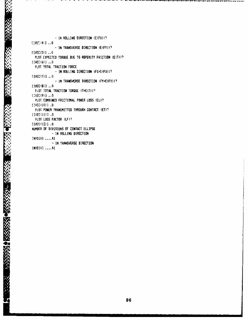
.
- IN ROLLING DIRECTION (ECFX))?[tVEC4)] .,O
- IN TRANSVERSE DIRECTION IE(FY))?[IVEC(51] ..0
PLOT EXPECTED TORQUE DUE TO ASPERITY FRICTION (E(T))?[IVEC(6)] ..0
PLOT TOTAL TRACTION FORCE- IN ROLLING DIRECTION (FX+EIFX))?
[IVEC(7)] ..0- IN TRANSVERSE DIRECTION (FY+E(FY))?
HIVEC(B)] ..0PLOT TOTAL TRACTION TORQUE (T+E(T))l
{[:VEC(9)) ..0
PLOT COMBINED FRICTIONAL POWER LOSS (EL)?
([VEC(IO)] .0PLOT POWER TRANSMITTED THROUGH CONTACT (ET)?
[IVEC(II)] .0PLOT LOSS FACTOR (LF)7
[EIVEC(12)1 .0
NUMBER OF DIVISIONS OF CONTACT ELLIPSE- IN ROLLING DIRECTION
ENYDIVI ,141
- IN TRANSVERSE DIRECTION[NYDIV] .... 41
JI
j 86
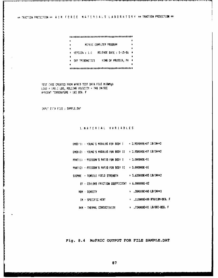
STRATION FREOI71ON ff A I R F 0 R C E M A T E R I A L S L A B 0 R A T 0 R Y **TRACTION PREDICTION*.
i&***i,ii**,ieot~iii**I***tmtii**
* MCFRIC COMPUTER PROGRAM* I
# VERSION : .C RELEASE DATE: B-15-8b *I *
* SKF TRIBONETICS KING OF PRUSSIA, PA #* I
*ii**l*l**I**#I * ll*** l*l***l*I*HI*******
TEST CASE CREATED FROM WPAFB TEST DATA FILE Mi8N9gO
LCAD = 140, LBS, ROLLING VELGCITY = 748 IN/SECA PIENT 'EMPERATURE = IV DEB. F
INP £'A FILE SAMPLE.DAT
1. MATER IAL VARIABLES
EMODI) - YOUNG'S MODULUS FOR BODY I = 2.950000E+07 LBIIN#*2
EMOD(2- YOUNG S MODULUS FOR BODY I = 2.950000E+07 LBIIN#*2
PRAT(l) - POISSON'S RATIO FOR BODY I = 3.OOOOOOE-O1
PRAT(2) - POISSON'S RATIO FOR BODY IT = 3.000000E-O1
SIMAE - TENSILE YIELD STRENGTH = 3.620000E+05 LBIIN#*2
EF -.COLOMB FRICTION COEFFICIENT = 6.OOOOOOE-02
ROM - DENSITY = .284000E+00 LD/INf*3
CM - SPECIFIC HEAT = .1I10000E+00 BTUILBN-DEG. F
AKN - THERMAL CONDUCTIVITY = .734000E+01 LB/SEC-DEG. F
Fig. 8.4 McFRIC OUTPUT FOR FILE SAMPLE.DAT
87
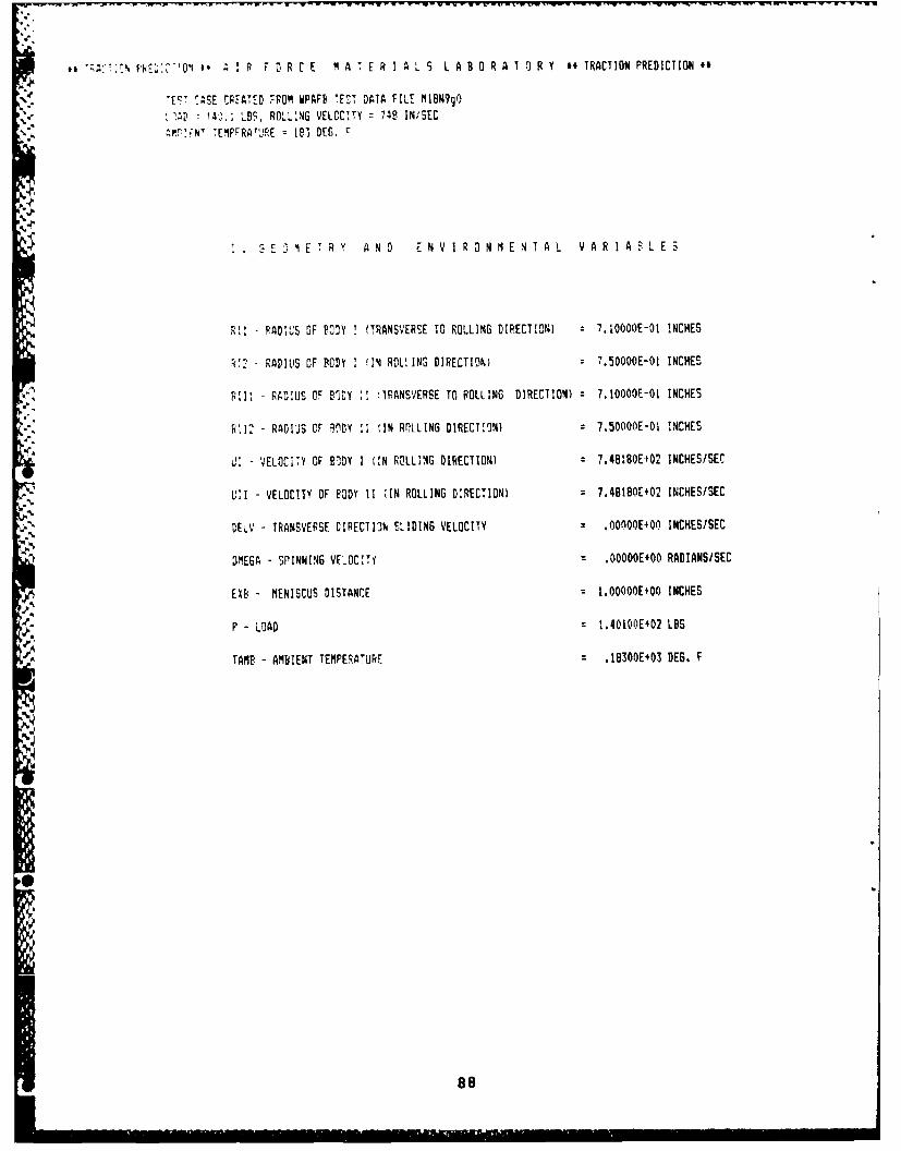
** ";"T2C KE ' OJ to A I R F D R C E M A T E R I A L S L A B 0 R A I 0 R Y of TRACTION PREDICTION *
'. ASE CREATED FROM WPAFB TEST DATA FILE MIBN99O
14l , D5, ROLLNG VELOCITY =748 IN/SEC^1PN r E.PFRA'JRE 183 DEG. F
I. 3 E" ME T R Y AND E NV IRON ME NT AL VAR I ASL E S
R1 - RADIUS OF BODY I (TRANSVERSE TO ROLLING DIRECTION) = 7.1OOOOE-O INCHES
- RADILS OF BODY I f1N RDLlING DIRECTION) = 7.50000E-01 INCHES
FlU - RADIUS OF BODY ,' :TRANSVERSE TO ROLLING DIRECTION) = 7.IO000E-OI INCHES
RII - RADIJS OF RODY I tIN ROLLING DIRECTION) = 7.5OOOE-OI INCHES
J- 'ELOCITY OF eDDY I (IN ROLLIG DIRECTION) = 7.48180E+02 INCHES/SEC
UI- VELOCITY OF FODY 11 IN ROLLING DIRECTION) 7.48180E+02 INCHES/SEC
DELV - TRANSVERSE DIRECTI3N SLIDING VELOCITY = .OOOOOE+O0 INCHES/SEC
OMEGA - SPINNING VELOCITY = .OOOOOE+O0 RADIANS/SEC
EXB - MENISCUS DISTANCE = I.OO0OE+O0 INCHES
P - LOAD = 1.401OOE+O2 LBS
TAMB - AMBIENT TEMPERATURE = .18300E+03 DEB. F
88

,TA.!;DN PREZir'0N * A : P F C R ' E x A T E R I A L 5 L A B 0 R A T O R Y H TRACTION PREDICTION
7(c'CWE CREATEr FROI WPAFE TEST DATA rILE IB19g9
= :4).I LBS, KL:LING VELOCITY = 748 IN/SECAr;!EN7 "RIFERAT , = tK DEG. F
,%
I1. R F I AN T V A R I A B L E 3
VISCS - OIL VISCOSITY AT OPERATING TEMPERATURE = 1.310000E 00 CENTISTOKES
SPGR - SPECIFIC GRAVITY OF OIL = 1.762700E00
FTAo - ABSCLUTE VISCOSITY - 3.4824BE-07 LB-SEC/IN*#2
LETA - TEMPERATURE VISCOSITY COEFFICIENT 1.O10OOE-02 IiDEG. R
ALFHAI - PRESSURE V:SCOSITY !NDEX : 7.4000E-05 INH*2/LB
CN - THERMAL CONDUCTIVITY OF LUBRICANT :.600000E-03 LBISEC-F
GBAR -- AVERAGE 5HEAR MODULUS 2.443690E+03 LBS/IN**2
TAII: - LIMITING SHEAR STRESS 1.260341E+04 LBS/IN**2
CF - SFECIFIC HEAT . 200000EOO 9TU/LBM-DE6, F
,l
I8
3~!
AD-AINS 450 TRACTION MODEL DEYELOPNENT(U) MRC BEARIUGS-SCF2/AEROSPACE KING OF PRUSSIA PR J1 I MCCOOL SEP 8?AFWdAL-TR-87-4879 F21615-84-C-5028
UNCLASSIFIED F/G 11/B U
EohEEEEohEoiIEhmhEEmhmhohhEE h h E E E E E E m o h mh EmEEmhhhohohEE
3.2
MICROCOPY RESOLUTION 'VEST 'EHAR
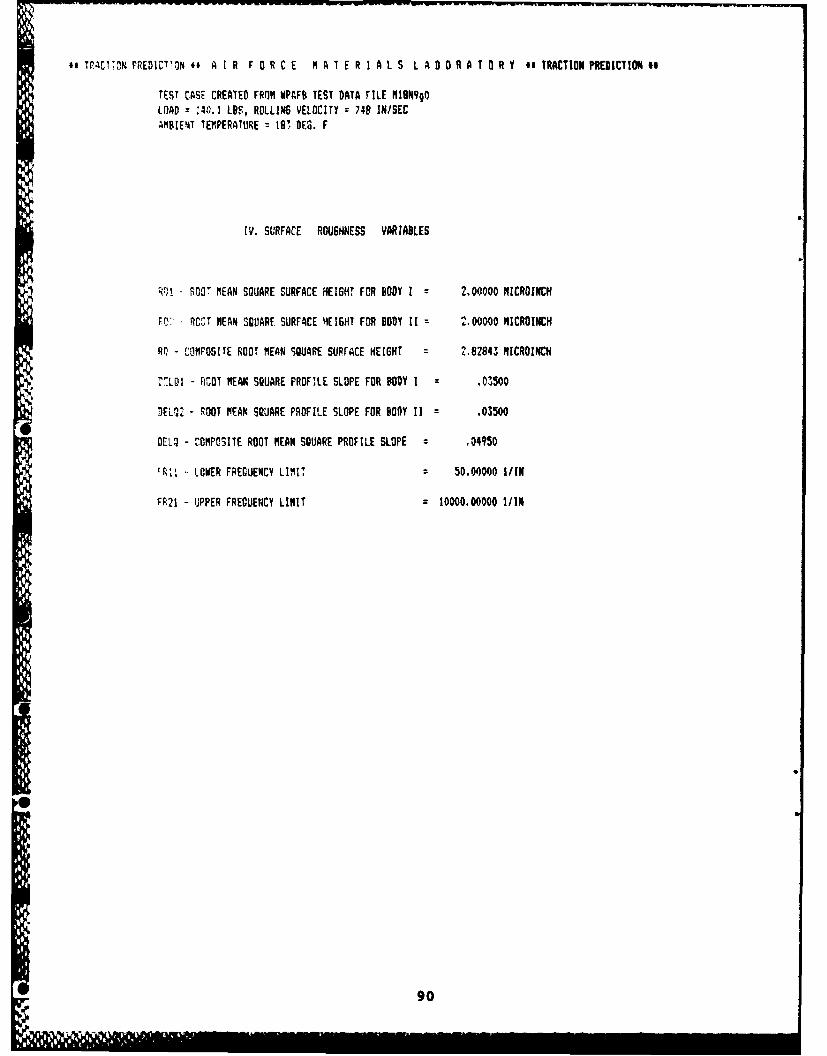
a. TPC17oN PREDICY'ON *# A I R F 0 R C E M A T E R I A L S L A B 0 R A T a R Y ii TRACTION PREDICTION 4
TEST CASE CREATED FROM WPAFB TEST DATA FILE MIN990LOAD = :4). LOS, ROLLING VELOCITY r 748 IN/SECAMBIENT TEMPERATURE = 18 DES. F
IV. SURFACE ROUGHNESS VARIABLES
Rf -- FO0 rEAN SQUARE SURFACE HEIGHT FOR BODY I = 2.00000 NICROINCH
; - RCOT MEAN SQUARE SURFACE HEIGHT FOR BODY II = 2.00000 NICROINCH
Rr - COMPOSITE ROOT MEAN SQUARE SURFACE HEIGHT = 2.62843 MICROINCH
"L01 - RSOT MEAN SQUARE PROFILE SLOPE FOR BODY I z ,03500
DEL 2 - ROOT MEAN SQUARE PROFILE SLOPE FOR BODY II = .03500
DELI - COMPOSITE ROOT KEAN SQUARE PROFILE SLOPE = .04950
-- LOWER FREGUENCY LIMIT - 50.00000 I/IN
FP21 - UPPER FREQUENCY LIMIT 10000.00000 1/IN
90
IIII11
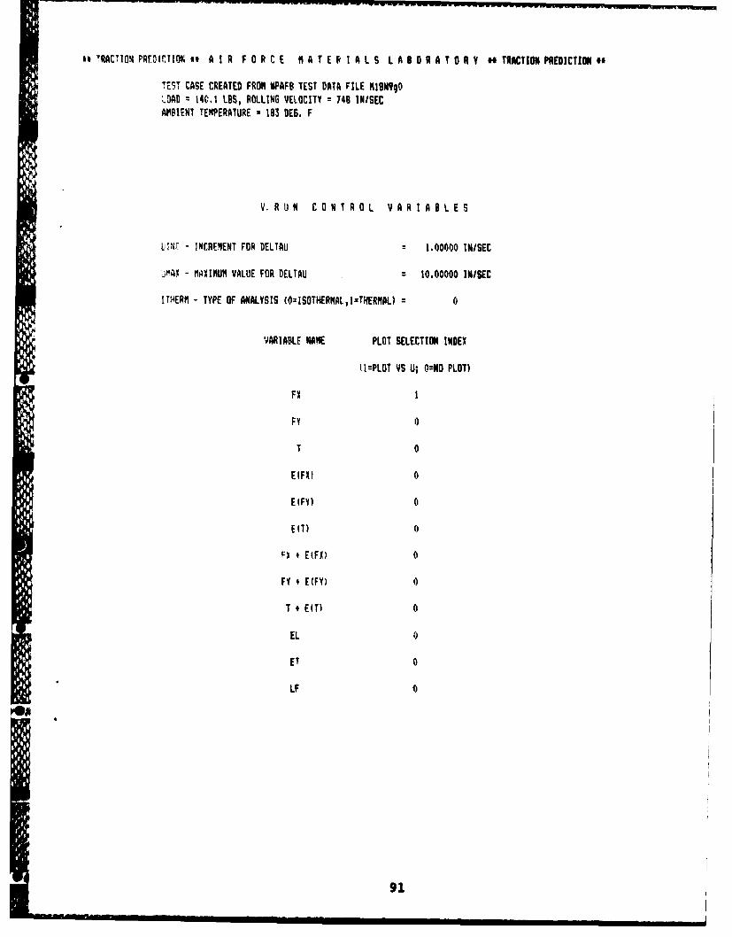
i*TRACTIO PREZICTTOK it A I R F 0 R C E H A T E RI A L S L A O R A T 0 R Y t* TRACTION PREDICTION to
TEST CASE CREATED FROM WPAFO TEST DATA FILE MIUNqO0LOAD m 140,1 LBS, ROLLING VEL.OCITY = 748 INISECAIBIENT TEMPERATURE z 183 BEG. F
V, RUN CONTROL VARIABLES
U,!N, - ]NCREMENT FOR DELTAU " 1.00000 IN/SEC
JMAW - MAIIMUM VALUE FOR DELTAU = 10.00000 IN/SEC
ITHERN - TYPE OF ANALYSIS (O:ISOTHERNAL,I:THERMAL) m 0
VARIABLE NAME PLOT SELECTION INDEX
'1=PLOT VS U; 0O0 PLOT)
FX 1
FY 0
T 0
E(FX) 0
EIFY) 0
ET) 0
F) + E(FX) 0
FY # E(FY) 0
T + E(T) 0
EL 0
ET 0
LF 0
91

*,TRACTION PREDICTION ## A I R F O R C E M A T E R I A L L A DO R A O R Y TRACTIONPREDICTION t
TEST CASE CREATED FROM WPAFB TEST DATA FILE hION990
LOAD = '40.1 LOS, ROLLING VELOCITY = 748 IN/SECAIDIENT TEMPERATURE 2 18 DES. F
HERTZ CONTACT PARANE TERS
AREA - AREA OF CONTACT ELLIPSE = 5.62472E-04 INCHES#02
DELTA - TOTAL ELASTIC APPROACH = 4.90480E-04 INCHES
SIMAO - MAXIMUM HERTZ CONTACT PRESSURE = 3.73619E+05 LBS/INn#2
A - CONTACT ELLIPSE SENIAXIS IN ROLLING DIRECTION z 1.36275E-02 INCHES
B - CONTACT ELL'PSE SE"IAIIS IN TRANSVERSE DIRECTION z 1. 1381E-02 INCHES
92
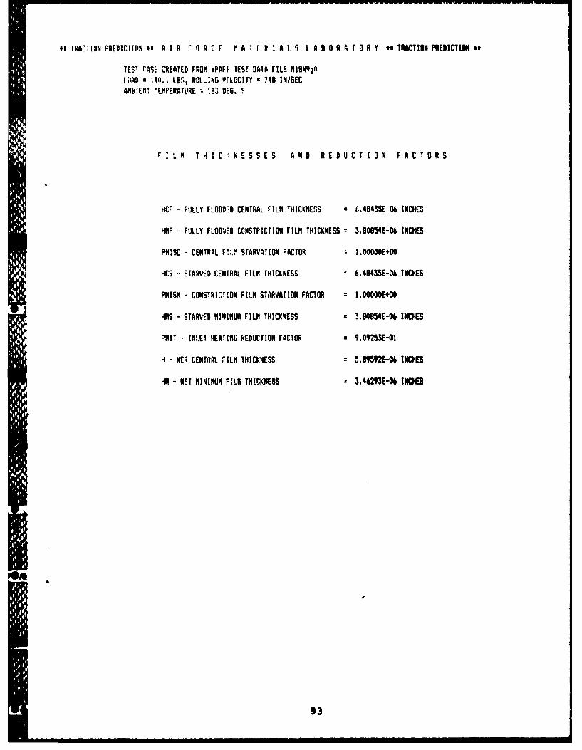
*' TRAC113N PREDICItIPN to A I R F 0 R C F 0 A I f R I A 1. S ( A 9 0 R A T 0 R Y ## TRACTION PREDICTION so
TEST rASL CREATED FROM WPAFi TEST DATA FILE NION990LPAD = 140. LDB, ROLLING VFLOCITY = 749 INISECAWIfEN! 'EMPERATURE = 183 DEG. F
I I Lm TH I C iNESSES AND REDUCT ION FACTORS
HCF - FULLY FLOODED CENTRAL FILM THICKNESS = 6.48435E-06 INCHES
HMF - FULLY FLOOVED CONSTRICTION FILM THICKNESS = 10,0854E-06 INCHES
PHISC - CENTRAL FiL STARVATION FACTOR tI.00OE+O0
HCS - STARVED CENTRAL FILM THICKNESS r 6.40435E-06 INCHES
PHISH - CONSTRICTION FILM STARVATION FACTOR I.000E+00
HMS - STARVED MINIMUM FILM THICKNESS Z 3,$854E-06 INCHES
PHIT - IN.ET HEATING REDUCTION FACTOR = 9.0925E-01
H - NET CENTRAL FILM THICKNESS m 5.B 9N-06 INCHES
RM - NET MINIMUM FILM THICKNESS = 3,46293E-06 INCES
9 3
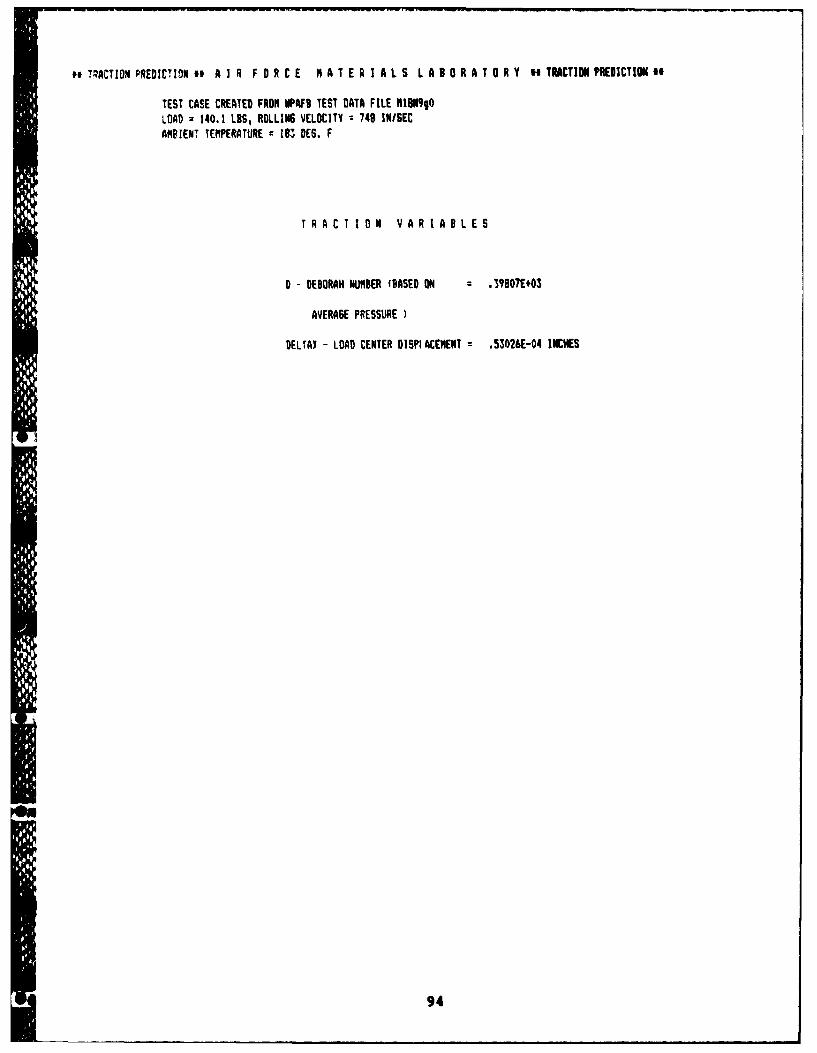
*TRACTION PREDICTION # A IR FOR C E MATERIALS LABORATORY ti TRACTIONPREDICTIONO
TEST CASE CREATED FROM WPAFB TEST DATA FILE MlO990LOAD 140.1 LUS, ROLLING VELOCITY z748 INISECAPPIENT TEMPERATURE = 83 DES. F
T RA C TIO0N VA RI A BLE S
D - DEBORAH NUMBER ESASED ON .39007E+03
AVERAGE PRESSURE )
DELTAY - LOAD CENTER DISPI ACEMENT = .53026E-04 INCHES
9 4
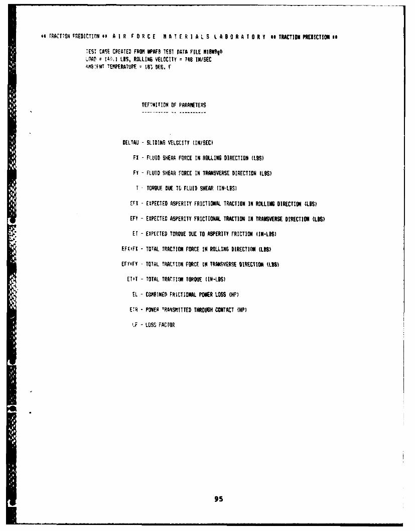
of tRACTTON PgEDICTIDN.# A I R F OR C E MA T E R I AL S L A8O R A T OR Y *OTRACTION PREDICTIONeo
.EST CASE CREATED FROM PAFB TEST DATA FILE NIRN9qO-iJ lAE 14,,. LBS, ROLLING VELOCITY = 748 INISEC%' FNT TEMPERATUPF. 183 DEG. f
OEF',NIT ION OF PARAMETERS
DELTAU - SLIDING VELOCITY (IN/SEC)
FX - FL-UID SHEAR FORCE IN ROLLING DIRECTION (LBS)
FY - FLUID SHEAR FORCE IN TRANSVERSE DIRECTION (LBS)
T TORQUE DUE TU FLUID SHEAR IIN-LBSI
EFX - EXPECTED ASPERITY FRICTIONAL TRACTION IN ROLLINS DIRECTION (LOS)
EFY - EXPECTED ASPERITY FRICTIONAL TRACTION IN TRANSVERSE DIRECTION IL3)
ET - EXPECTED TORQUE DUE TO ASPERITY FRICTION (IN-LS)
EFI0FX - TOTAL TRACTION FORCE IN ROLLING DIRECTION (LBS)
EFY4FY TOTAL TRACTION FORCE #11 TROXSVERSE IIIRETION (LBS)
ET.T - TOTAL TRArTION TORQUE (IN-LBS)
EL - COMBINED FRICTIONAL POlER LOSS (HP)
ETR - POWER TRANSKITTED THROUGH CONTACT (HP)
I.F - LOSS FACTOR
95

ii f~t7'Ck PREDU'r 7 R '0 P C E M A TER I A LS L ABO R AT ORY *# TRACTION PREDICTION##i
":S CASE CREATED FROM WPAFB TEST DATA FILE 41ON9gO"A = 340-1 IBS, ROLLING VELOCITY =748 INISEC
AMB17-NT TEM~PERATURE =183 DES. F
PLA. FE EFX EFY ET FX+EFX FY+EFY T+ET EL ETR IF
.00')..-E~. .0,)E+00 .0IE+00 OO00 .OOE+00 .OOE+00 DOOE400 .00E+00 .OOE+00 .00E+00 .OOE400 .00E400
1.0 3~E0 0E+00 -1.60E-19 1.86E-01 JC,E*O -9.96E-04 3.19E540 .OOE+00 -9.96E-04 4.83E-04 3.625-01 I.34E-03
2.~ .02+K~ 'E~(~i4- 1 ,04E-04 Oo4+0 00.OE+00 5.02E#00 .00E+00 3.34E-20 I 5E-03 E.9-0 27E-03i
...(00 5.98E+r0, .IE+00 -4.48E-19 5.87E-08 .GuE400 Df0E+00 5.98(00 O0OE+00 -4.48E-19 2.72E-.03 6.78E-01 4.OIE-03
i.0,10~ 6.4?E+,If *0 o+0;) -1.51E-16 3.30E-11 .00E40(, .OOE+00 6.42E#00' .00E+00 -1.51E-18 3.89E-03 7.26E-01 5.35E-03
5:W0 .61K+0 .'E0 -1.5E-18 1.46E-14 OOEEOA .045.00 6.63E40 O )0E+00 -1.53E-l8 5.03E-03 7.52E-01 6.68E-03
6.00o c 75T0,GWIV 2.2?E-198 1.05E-17 -.067+00 .OtE+00 6.75E+00 OO0E+00 2.29E-18 6.13E-03 7.65E-01 8.02E-03
*' O .E~' . 0E+0f 0 E1 5.88F-21 .OOE+00 .00E+00 6,91E+00 .00E+00 1.71E-18 7.22E-03 7.72E-01 9.36E-03
gj~~S+) ;:t' -. ~-8 3.31E-24 00['400 .OOE4O0 6.85E#00 .OOE+00 -1.13E-18 8.30E-03 7.77E-01 1.075-02
2-;t 68E0i .4 0 23-19 1,86E-27 .04500 MOEWO 6.88E+00 .0OE+00 2.03E-18 9.38E-03 14.60E-01 1.20E-02
-;.001, to.90E+IY. .1KOE*c .:E~ 1.05E-30 .00E400 MW0O0 6.90E+00 .OOE+00 1.16E-16 1.04E-,02 7.02E-01 1.114E-02
96
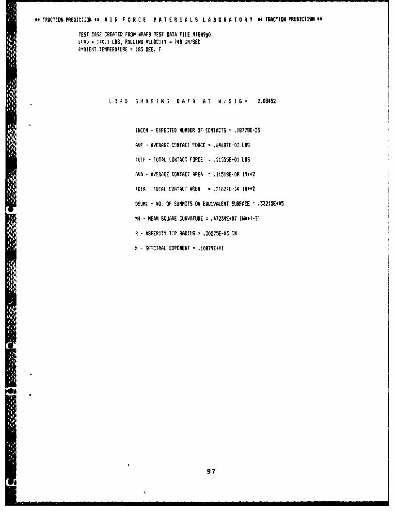
## TRACTIONPREDICTION i A IR F 0 R C E MA T ER I A L S L A B R A T 0R Y 1# TRACTION PREDICTION'
TEST CASE CREATED FROM NPAF9 TEST DATA FILE MIBN990LOD = 140.1 LBS, ROLLINS VELOCITY = 748 INISEC0M3IENT TEMPERATURE = 183 DES. F
L 0AD SHAR ING DATA AT H/ SI 6= 2.08452
ZNCON - EXPECTED NUMBER OF CONTACTS = .I877BE-25
AVF - AVERAGE CONTACT FORCE = .64687E-03 LBS
IOTF - TOTAL CONTACT FORCE : .21555E+01 LBS
AVA - AVERAGE CONTACT AREA = .I151BE-08 IN'*2
TOTA - TOTAL CONTACT AREA = .21627E-34 INH2
OSUMI - NO. OF SUMMITS ON EQUIVALENT SURFACE = .33215E+05
M4- MEAN SQUARE CURVATURE = .47234E+07 INW*f-2)
R - ASPERITY TTP RADIUS = .30575E-03 IN
K - SP'CTRAL EXPONENT = .10879E+01
97
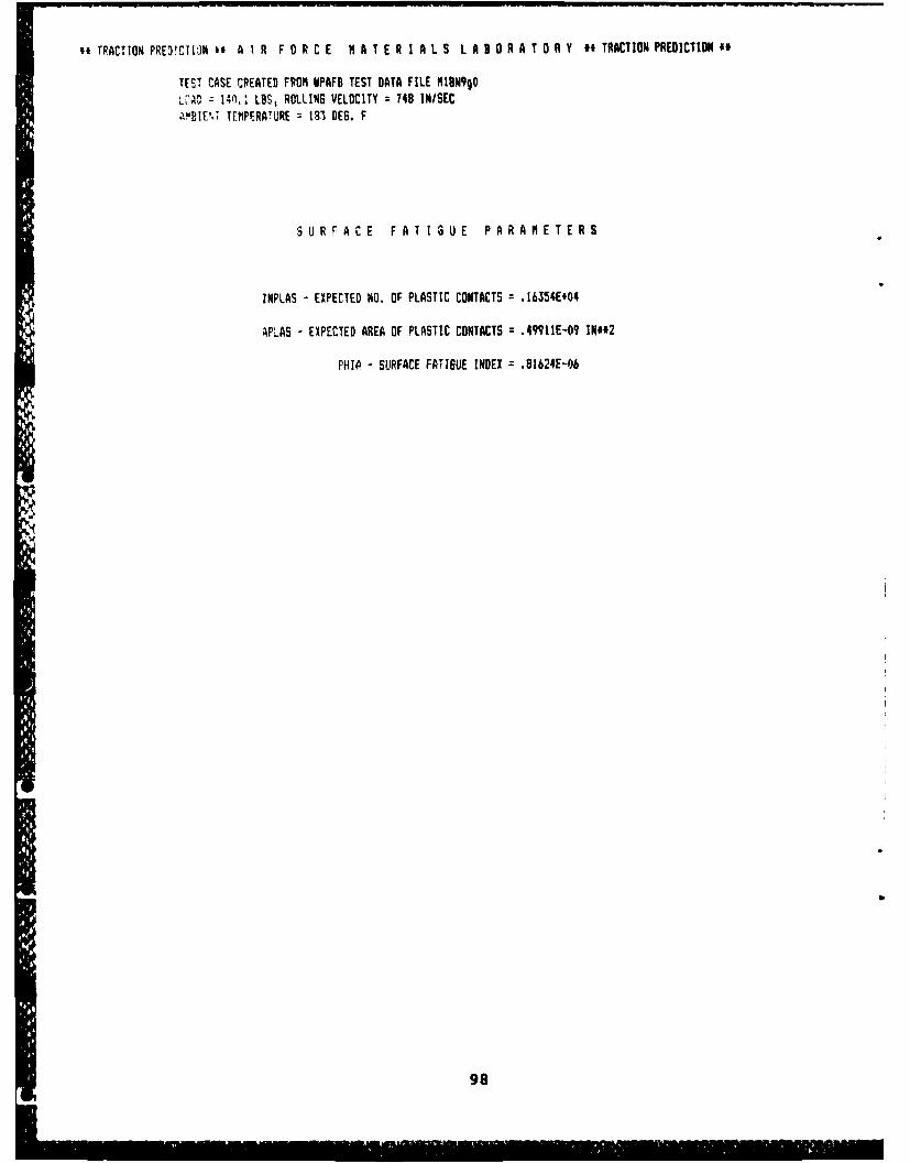
u.TRACTION PRED!CTION * A I R F OR C E H AT E R I AL S L ABOR A T OR Y *4 TRACTIONPREDICTIONO'
TEST CASE CREATED FROM WPAF8 TEST DATA FILE RION9gO
z 14)0' LS, ROLLING VELOCITY= 749 IN/SEC
A41E'.- TEMPERATURE = 183 DEG. F
SUR ACE FAT IGUE PARAMETERS
ZNPLAS - EXPECTED NO. OF PLASTIC CONTACTS = .16354E+04
APLAS - EXPECTED AREA OF PLASTIC CONTACTS = .499I1E-09 IN*#2
PHIA - SURFACE FATIGUE INDEX = .81624E-06
98
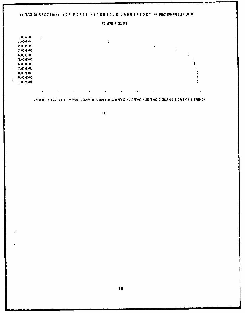
,TRACTIO PREDIC T1DNA ,R F RC EM AT ER IA L S'L A B R A T 0RVTR ACTIOhPRED CTON~
FX VERSUS DELTAU
1.000)E00'
2.fl)Ofl+Oo
7.030E+00
9j. OOE+00
9. OOOE+OOL.OOOE4OI
.OOOEt+f. 6,896E-01 !,I37?E.')O 2.069E+00 2.758E+00 11.448E+00 4,1747E+00 4.827E+00 5.516E+00 6,206E+00O 6.896E#00
FX
99
2. Use a commercial editor or word processing package (such
as WORDSTAR in non-document mode or WORD in non-
formatted mode) to edit the data in the new file.
As already noted, the required input data file structure is
illustrated in Fig. 8.3. In setting up the file structure,
effort has been taken to make editing of the input data possible
without reference to a manual. To this end, all of the headings,
variable descriptions, units and symbols, and blank or dashed
lines shown in Fig. 8.3 are built right into the data file.
(Important Note: Since the program uses fixed format FORTRAN
read statements, it is vital that the user edit only the data
fields. None of the headings, variable descriptions, blank
lines, etc. should be deleted or changed in length because the
program expects to read the data in a specific location).
The input parameters are organized into 6 general categories:
title information, material data, geometry and environmental data,
lubricant data, surface data, and run control data. The input
data fields are identified by the characters A (Alphanumeric)
F (Floating Point) and I (Integer) indicating the type of data
expected. Alphanumeric data consists of any combination of num-
rbers letters or symbols. As noted, the program output produced
by this input file is included as Fig. 8.4.
pa
100@4

9.0 TRACTION TEST PROGRAM
As part of the contract effort, a set of four lubricants were
selected, fluid samples were acquired and a traction test program
was designed and performed within AFML, using an Air Force owned
traction rig. The dual purpose of the traction test program was
to provide input data for McFRIC and to evaluate its predictive
accuracy.
9.1 Traction Rig and Test Variables
The parallel axis, two disc traction apparatus used in this
study is shown schematically in Fig. 9.1. A full description is
given in Smith [25]. A characteristic of the rig is that it
requires only a small amount (400 ml) of the test fluid. The
crowned discs are separately driven via independent drive
transmissions and variable speed motors. A normal load is
applied by means of a pneumatic load system. A variable speed
pump is used to circulate the oil. A heat exchanger in the inlet
line maintains the lubricant at the desired temperature.
The discs are made of 52100 vacuum degassed alloy steel with
a hardness of 60-63 Rc. They are 1.5 in. in diameter. In the
test program the disks had a lateral or crown radius of either
0.71 in., providing a nearly circular contact zone, or 6.22 in.
providing a 4:1 aspect ratio, i.e., ratio of the major-to-minor
axes of the contact ellipse.
101

mohj oto a
N.Ud Aims
0NMMJP
4fl1A* A
Fig. 9.fFLTATO I
r~sy aete102
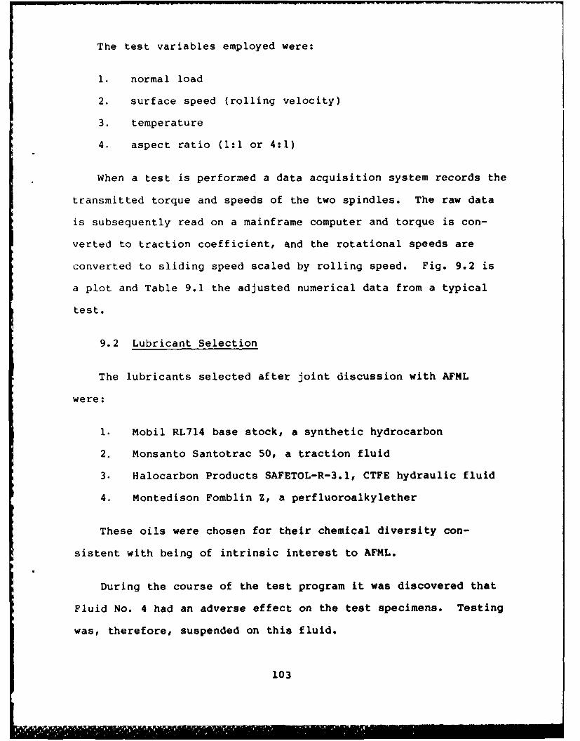
The test variables employed were:
1. normal load
2. surface speed (rolling velocity)
3. temperature
4. aspect ratio (1:1 or 4:1)
When a test is performed a data acquisition system records the
transmitted torque and speeds of the two spindles. The raw data
is subsequently read on a mainframe computer and torque is con-
verted to traction coefficient, and the rotational speeds are
converted to sliding speed scaled by rolling speed. Fig. 9.2 is
a plot and Table 9.1 the adjusted numerical data from a typical
test.
9.2 Lubricant Selection
The lubricants selected after joint discussion with AFML
were:
1. Mobil RL714 base stock, a synthetic hydrocarbon
2. Monsanto Santotrac 50, a traction fluid
3. Halocarbon Products SAFETOL-R-3.1, CTFE hydraulic fluid
4. Montedison Fomblin Z, a perfluoroalkylether
These oils were chosen for their chemical diversity con-
sistent with being of intrinsic interest to AFML.
During the course of the test program it was discovered that
Fluid No. 4 had an adverse effect on the test specimens. Testing
was, therefore, suspended on this fluid.
103

TRACTION DATA FOR MOBIL RL-71-4 LUBE549 RPM %Load=55.5 lbs (151392 psi) ! TooaSDiameterinl.500 !n z Crown Rod:106 31 &6.4 to
TC(u) Material a52100 Voc Degas Rc 60-63 Stel!)at* File K0808PI
0
010

TABLE 9.1 ADJUSTED TRACTION DATA POINTS
TRACTION DATA FORl MOBIL RI -114 LURF549 RPM :Load=55.5 Lbb. (1'Jd392 p~si) :remp=8o vOiameter=1.500 in : Crown Radii=6e31 6.14 InMaterat . 52100 Vac Degas Rc 60-63 Steel.Data Fite K0808PI
SLIP/R0L1 TRACTION COEFF.+.223247936558 **027674469013'.214825449325 +.027223613875'.204092902270 +.026952478819**189495552626 '.026637741805*,i7aM3834729 +*026205821547* .170185391809 *.025993459509+.160154092165 *e02580644.0712+.149261595311 '.0252031515R0'.134189667323 *.024448551508*.1l25396658076 *.023883652569*.118138554873 +.023285083033'.108101322613 +o022682200608+.091946167213 +.021420221116*.081469149176 *.020380410023*.071183689490 *o019564074996*.0624609428466 +oo1S179835505+.041911851497 *.016020874931'.035990053183 +.013874833549'.026866994513 +o012077675182'.018988376614 +.009338437182'.006398940062 +.0033455750694.000000000000 ,0000000000000-.007104808654 -.003715537039-.016589580465 -.008085418931-.025369241611 -.01058(427440-.034220311411 -.012687189245-.05~0478183774 -.015424554585-e061473280307 -.016647504835-oU69721B4006 -0017 6 7Q981613-o0140001743749 -.018523279248-,09~4994514238 -0019916209915-.10542753R995 -*020679601353-. 114829*77354 -.021301196610-.124677192638 -.021769360098-013,5011051J941 -.022631391080-,14986881057235 -.02368.4925032-.158470937793 -.02392V,7R0125-,167301i547179 -o0242414517R3-.17bJ3O18bbi -o024387033208-.193437713521 -.02500'!052?(,2-,2312814322n72 -. 02 ,277940731-. 211(,16783243 -. 0257FS'698940
105
9.3 Lubricant Properties
Shear Modulus G and Average Limiting Shear Stress Tc
The extreme conditions of pressure, transit time and shear
rate met in a typical EHL contact preclude the direct measurement
by ordinary laboratory techniques of the properties G, Tc and the
average viscosity n under relevant conditions. They must, there-
fore, be deduced directly from traction measurements.
Following Tevaarwerk and Johnson [4J it is assumed that trac-
tion curves of the type shown in Fig. 9.3 are available at or
*close to the loads, speeds, aspect ratios and temperatures of
interest. These tests are termed simple sliding tests because
there is no imposed spinning velocity or transverse sliding velo-
city. Only the sliding velocity in the rolling direction, Au, is
varied. The maximum traction coefficient is reached at high
sliding velocities. At sufficiently high sliding speeds the
fluid will be plastic so that the traction force Px will be the
product of the average limiting shear force Tc and the contact
area wab, i.e.,
Fx = wabrc (9.1)
Dividing Fx by the applied load P gives the maximum traction
coefficient Pmax:
Pmax = xab~c/P (9.2)
106
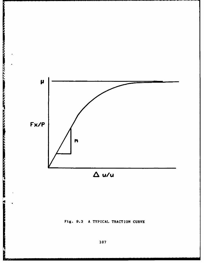
Fx/P
u/U
Fig. 9.3 A TYPICAL TRACTION CURVE
107

Using Eq. (9.2) Tc may be computed as:
tc = maxP/wab (9.3)
For high Deborah numbers the oil will act purely elastically
at low sliding rates. Tevaarwerk and Johnson [4] show that in
this regime the resultant shear stress integrated over the ellip-
tical contact area gives a force of
Fx = 8/3 (a 2b/Ph)G 0 Au/u (9.4)
wherein G, the composite shear modulus of the fluid and con-
tacting surfaces, is assumed to be constant through the contact.
P- Fx/P is, therefore, linear with Au/u and has slope:
m E 8/3 a2b/Ph S G (9.5)
By measuring the slope a of the traction curve in the high
Deborah number regime one may thus compute G as:
G = 3/8 Phm/a 2b (9.6)
Inasmuch as the solid surfaces as well as the fluid deform
elastically, this elastic modulus value represents the combined
deformation of the composite fluid/solid system.
For low Deborah numbers the oil in the interface behaves as a
., Newtonian fluid, i.e., the shear stress is related to sliding
Oft velocity as:
Is10
i . .M !I
= n Au/h (9.7)
Considering isothermal conditions but using Barus' law for
pressure dependence of viscosity, Fx is obtained as:
Fx = jjTdxdy = JJn(p)dxdy AuL/h (9.8)
= ' a b n Au/h
= u r a b 7/h 0 Au/u
where n is the average viscosity across the contact ellipse. In
this case P = Fx/P will also be linear with Au/u, but with slope
m given by
m = u r a b u/hP (9.10)
For intermediate Deborah numbers the traction curve at low
shear rates will depend jointly on the viscosity and shear modu-
lus.
At intermediate shear rates the shape of the traction curve
will depend jointly on the values of n, G and Tc , with their
relative influence a function of Deborah number. At high Deborah
numbers the traction curve shape at intermediate sliding veloci-
ties depends on G and Tc" At low Deborah numbers, intermediate
sliding velocity behavior depends on ii and Tc.
One conceivable approach to estimating the lubricant parame-
ters would be to use a least squares fit to an experimental trac-
109
tion curve. In this approach, n, G and cc are estimated as the
values which minimize the sum of the squared deviations of the
predicted and actual curves. This approach could be prohibiti-
vely time consuming inasmuch as the program would have to be run
repeatedly for various trial values of the lubricant parameters.
As a practical alternative the following approach was adop-
ted: 1) T c is computed from Eq. (9.3), 2) G is computed from
Eq. (9.5) on the assumption that the traction curve at low
sliding speeds is elastic, 3) n is taken at the value based on
its ambient viscosity value and Barus' equation integrated over
the contact pressure.
These values are used in the computation of the Deborah
number as discussed in Section 2.0. If the Deborah number is
large enough, n is irrelevant since the initial slope depends on
G only. If Deborah number is small, n can be adjusted as needed
to agree with the measured slope a using Eq. (9.10).
9.4 Further Lubricant Properties
In addition to G and cc, it is necessary, both for the design
of the traction tests and for input to McFRIC, to know six pro-
perties of each lubricant as a function of temperature. These
properties are:
viscosity 1
temperature viscosity coefficient 0
110

pressure viscosity coefficient a
specific gravity SPGR
specific heat c
thermal conductivity Kf
A computer program entitled MATPROP and written in Fortran 77
for an IBM PC and compatibles, was developed to compute the
required values at whatever temperatures T (OF) are of interest,
for the three oils used in the test program. The relationships
employed within MATPROP are given below.
9.4.1 Viscosity
The Walther-ASTM equation was used to relate viscosity n (cs)
to temperature (OF) as follows:
log(n+0.6) = exp[K-clnT] (9.11)
where K and c are fluid dependent constants. By substituting n
at two temperatures, it was possible to solve for the constants K
and c for each oil. The values thus determined are listed below:
Lubricant K c
RL-714 23.71805 3.55330Santotrac 50 24.689883 3.7017861CTFE 43.66862 6.82620
The viscosity values used in determining these constants were
taken from 126], 137] and 128] respectively for the three oils.
1; 111
9.4.2 Temperature Viscosity Coefficient
Given the viscosities nI and no , corresponding to the two
temperatures T1 and To , the pressure viscosity coefficient 0 is
calculable as
= -in(nl/n 2 )/(Ti-TO ) (9.12)
To find 6 at an arbitrary temperature T, T1 was taken as
T+20 0 and To as T-20. nI and n2 at these two temperatures were
then computed from Eq. (9.11) and 0 calculated from Eq. (9.12) as
n = n(n(T+20)/n(T-20)j/40 (9.13)
9.4.3 Pressure Viscosity Coefficient
RL714
A graph of a vs. T supplied in [261, was fitted by the
following equation:
a = exp (6.203294E-6 T-0.00363T-8.899781 (9.14)
SANTOTRAC 50
Values of a at three temperatures were given in [291 for a
traction fluid known to be Santotrac 50. The following curve fit
was developed:
a = exp[-0.0057T - 7.88581 (9.15)
112
0 ' ? W

CTFE
The following linear approximation was developed to a curve
given in [31].
a = 1.82287E-4 - 6.1598E-7eT (9.16)
This equation is used in program MATPROP. It does not
reflect the change communicated in [30] that a at 275 0 F for CTFE
is 4.276E-6 in2/lb. The program is believed to be valid for
T,180 0F.
9.4.4 Specific Gravity
RL714
The equation given in [26] is:
SPGR = 8.177 - 1.13E-3 0 T (9.17)
The following equations were obtained as least square fits
to data in [27] and [281.
SANTOTRAC 50
SPGR = 0.9237 - 3.45E-4T (9.18)
CTFE
SPGR = 1.9303 - 9.3091E-4T (9.19)
1134

9.4.5 Conductivity
RL714
The following equation was given in [26].
K = (0.8l3/(12*SPGR)*(l.O-3E-4(T-32)*O.2161 lb-sec/PF (9.20)
The following equations were obtained as least squares fits:
SANTOTRAC 50
K = 0.061-lE-5T T 4 200OF
= 0.065-3E-ST T > 200OF
CTFE
K = 0.01016 - 81.647E-6T
9.4.6 Specific Heat
RL714
The following piecewise linear fit was obtained:
c = l.175E-3T + 0.405 T<200OF
c = O.210E-3T + 0.598 T>200OF
SANTOTRAC 50
c = 6.15E-4T + 0.3840
114
CTFE
The value c = 0.20 was used independently of temperatures.
9.5 Test Design
The range of variables used in the tests was limited by the
maximum load that could be safely applied to the rig (140 lbs),
and by upper and lower limits on the rotational speeds (500 rpm
and 10000 rpm). Three temperatures were chosen: 800 F, 180°F and
280'F. Three values of the maximum Hertz stress were used: 50
ksi, 206 and 366 ksi. These stresses were achieved using loads
of 24.7 and 139 lbs with the two specimen crown radii. Using the
lubricant properties relevant to the temperature, the rolling
speeds were calculated using computer program TRIBOS [19] so as
to give three values of constant film thickness for each tem-
perature regardless of load or aspect ratio. This could not
always be achieved because of the physical constraints cited
above.
Tables 9.2 through 9.4 show for each combination of load, tem-
perature and aspect ratio the test number assigned by AFML, the
* required rolling speed (in/sec) and the computed film thickness
(pin). The entire set of tests at 280°F were eliminated for the
CTFE fluid because of concern about disk damage at the low calcu-
,S lated film thickness. A few other tests had to be discontinued for
various reasons accounting for some missing cells in the test matrices.
115

> 80 0 0 SO SO
z' Z 0 N 0lN 40 a
no
IL-
0 0 0I a a N N N I lC
0 o- - N.x x L
N 0 " 0
I 0
J. _jI
00
0~ *. I010 0 N1 NN 4" z
x x
0 0 0L 0 L Q
0 0 in
i - 1
ON z
N C)
a. p)______1 116a
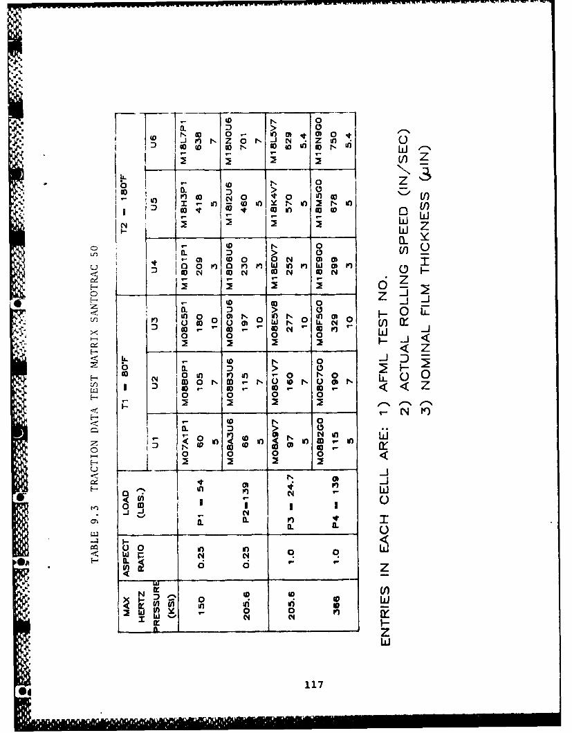
0
(D rl Go 0 n m r
0 *.z 0 r N Z00 jf
b 0 0
OD 0 0nin In
I~ I-
C 2 2 0 _
-0 LL0
if) 0 0) fl g 0 n o
0 0 0 0 w
0L 0. -OD10i) flu 0- LL
N 0 0 0 ) 0
M 0 N 0
-40 0 0 0
iN r4
N i Id0Of W I i If)
D (D (D IO
IL ~a. Ma. IL
u 0 n iwN N CI6 o d
-lii
ND ID W
01 d inF)I~
117
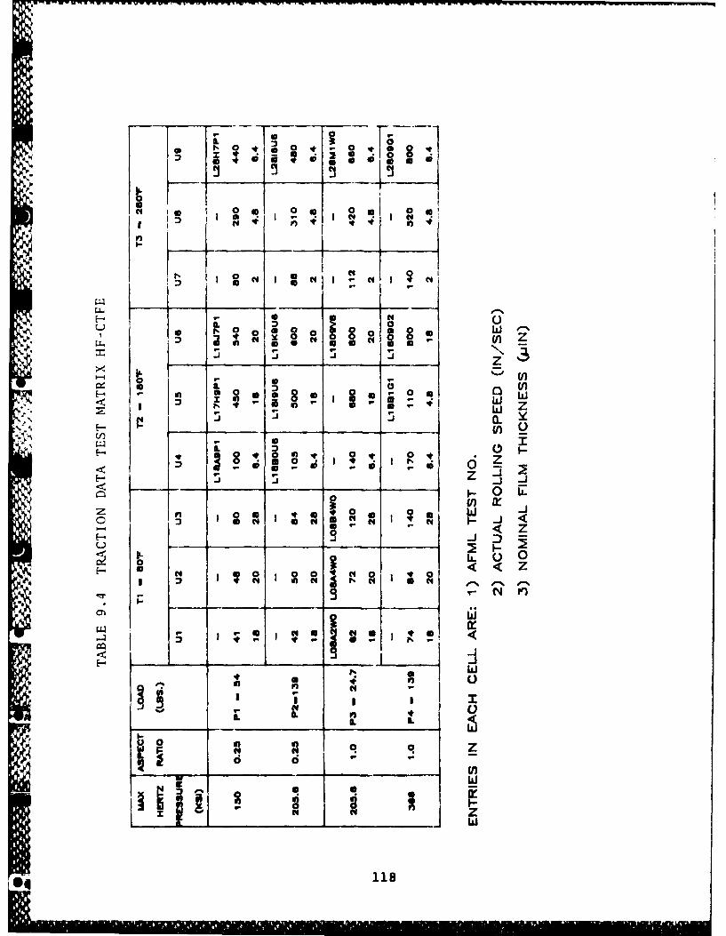
1,. 1p0 * * 0 0 - aq 0 0
p. ja. C-4 MI (
a s 0 0 .1 06'0
0 " 0V
in a~ 0 _ _ 8_ _
In, - go-I ~ (.ft rCr
is 4. ~ Ix 8 -~ 0 0 0 -)
I~ - rr
a 61 ' (4 (
N -
LL~ L
00
liei
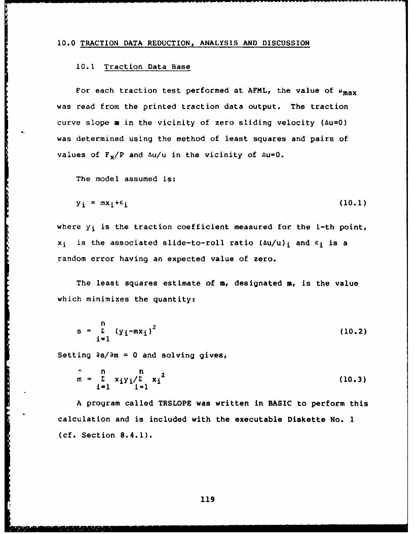
10.0 TRACTION DATA REDUCTION, ANALYSIS AND DISCUSSION
10.1 Traction Data Base
For each traction test performed at AFML, the value of Pmax
was read from the printed traction data output. The traction
curve slope m in the vicinity of zero sliding velocity (Au=O)
was determined using the method of least squares and pairs of
values of Fx/P and Au/u in the vicinity of Au=0.
The model assumed is:
Yi = mxi+Ci (10.1)
where Yi is the traction coefficient measured for the i-th point,
xi is the associated slide-to-roll ratio (Au/u)i and Li is a
random error having an expected value of zero.
The least squares estimate of m, designated m, is the value
which minimizes the quantity:
ns (Yi-mxi) (10.2)
i=l
Setting as/am = 0 and solving gives,
n nm xiyi/Z x i (10.3)
i=l i=l
A program called TRSLOPE was written in BASIC to perform this
calculation and is included with the executable Diskette No. I
(cf. Section 8.4.1).
119

Table 10.1 is a data form used to compile the data for each
traction test into a data base. With the data base software
system used to store and manipulate these data, it was possible
to specify certain fields by a formula relating the value of the
field to the values specified in one or more of the other fields.
The calculated fields are denoted by an asterisk in Table 10.1.
The formula used to compute these fields is given to the right of
the colon at the end of the field name. Specifically, the shear
strength and shear modulus are computed from Eqs. (9.3) and (9.6)
under the supposition that the fluid behaves elastically in the
low slip region and plastically at high slip. It is further
*assumed that the asperity contribution to traction is negligible.
Based on the computed film thicknesses relative to the surface
roughness (roughly 2 oin) this was almost certainly the case for
all but a few of the CTFE tests.
Tables 10.2 through 10.4 give the complete data base contents
for each oil. The column headings correspond to the field names
on the data form, but have been truncated in some cases.
These data were used to prepare input files for program
McFRIC. The program was run primarily in the isothermal mode
unless the AFML plots showed a clear indication that traction
diminished with sliding speed. After a series of trial runs
showed that the results changed negligibly for larger values of
NX and NY, the number of divisions of the contact ellipse were
taken as NX - NY - 41.
120
F M I . . .I ' ~~i ' .. ..
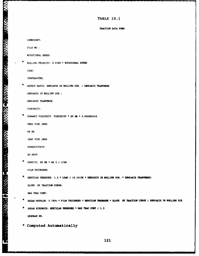
-- - - - - - - - -
TABLE 10. 1
TRACTION DATAF4
LUBRICANT:
FILE NO.:
ROTATIONAL SPEED:
* ROLLING VELOCITY: 0.0785 * ROTATIONAL SPEED
LOAD:
TEMPERATURE:
* ASPECT RATIO: SEMIAXIS IN ROLLING DIR. / SDIIAXIS TRANVERSE
SE!4IAXIS IN ROLLING DIR.:
SEMIAXIS TRAIIVERSE:
VISCOSITY:
DYNAMIC VISCOSITY: VISCOSITY * SP GR 0.000000145
PRES VISC INDX:
SP GR:
TEMP VISC INDX:
CONDUCTIVITY:
SP HEAT:
* DENSITY: SP GR * 82.5 / 1728
FILM THICKNESS:
*HERTZIAN PRESSURE: 1.5 *LOAD / (3.14159 * SDIIAXIS IN FMLLINO DIR. *SDIIAXIS TRANVERSE)
SLOPE OF TRACTION CURVE:
MAX TRAC COET:
*SHEAR MDULUS: 0.7854* FILM THICKNESS * NERTZIAN PREhSUhEK SLOPE Of TRACTION CURVE / SEWAXIS IN ROLLING DIR.
*SHEAR STRENGTH: NERTZIAN PRESSURE * NOX TRAC CODF / 1.5
DEBORAH 1O:
*Computed Automatically
121
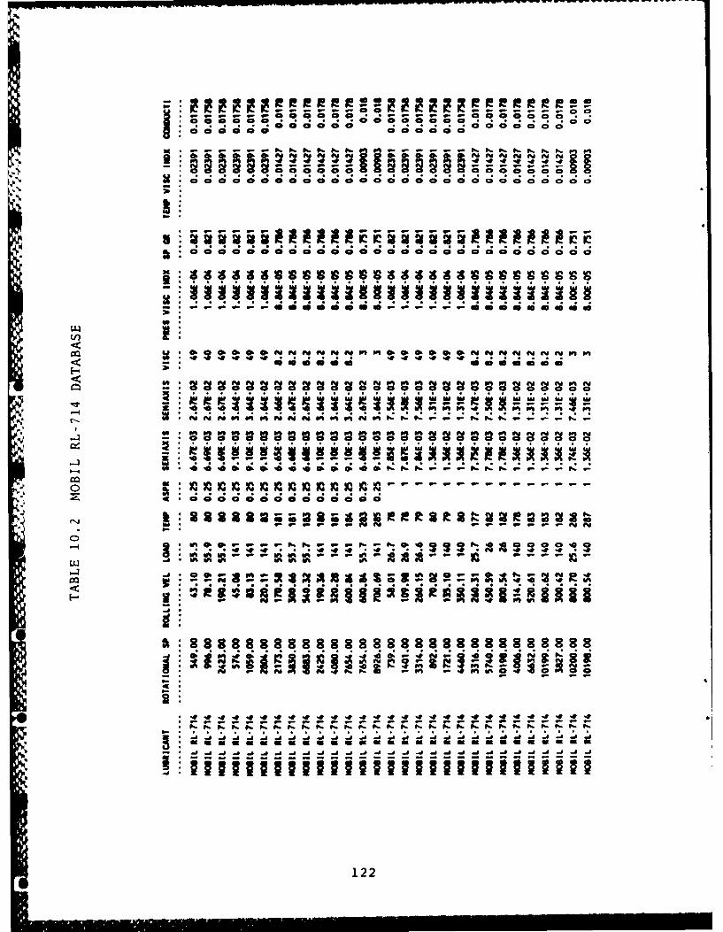
8:00000 0 0 0
- -- . " - - -n '.V .-. - - - I
42 o a 000C
C;C I C ;C ;C ; ;C ;C ;C D ;C ;C ;C ;C
-. -- -- -- -- -- -- - -
In 0 0 0 00 0 0
It 0 0 1,00 4 U00U0040 00
122;
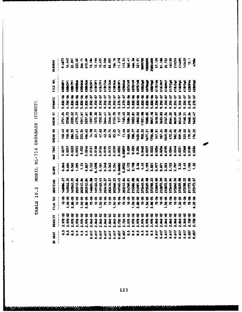
.o 0!N 4"N! 2. .~ 8 . * ...
u I'- -K IQ
. .- -. . . . . . . . . . . .- --.. .- . .O
000
ooH oC;C C, ,40 4' ;tjci4 A04C
0*
.~ N N N 3 4 4CD.~~~~~~ ~ ~ ~ ~ N N . .' .h . N .
0 !2 2!
* 4* Z Z* 4* .* N p. . . . .* .* .* .* .* .* . . . . . .
@ 0000044444444 00; 004444;44;
123
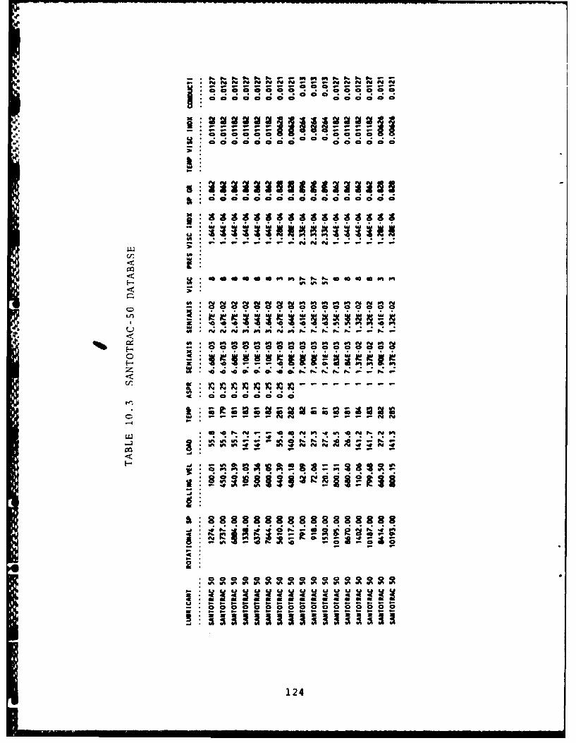
C3 caao-
40 a -- -- aao .T- 00 0 40- 0 a -0
CD000?000 . . . 0 0
0 00 0 0 0 a. 00, 0001 - P.
-a -~ - -. --- -a -~
CVV
0 a 0 0 0 0 0 0
C124
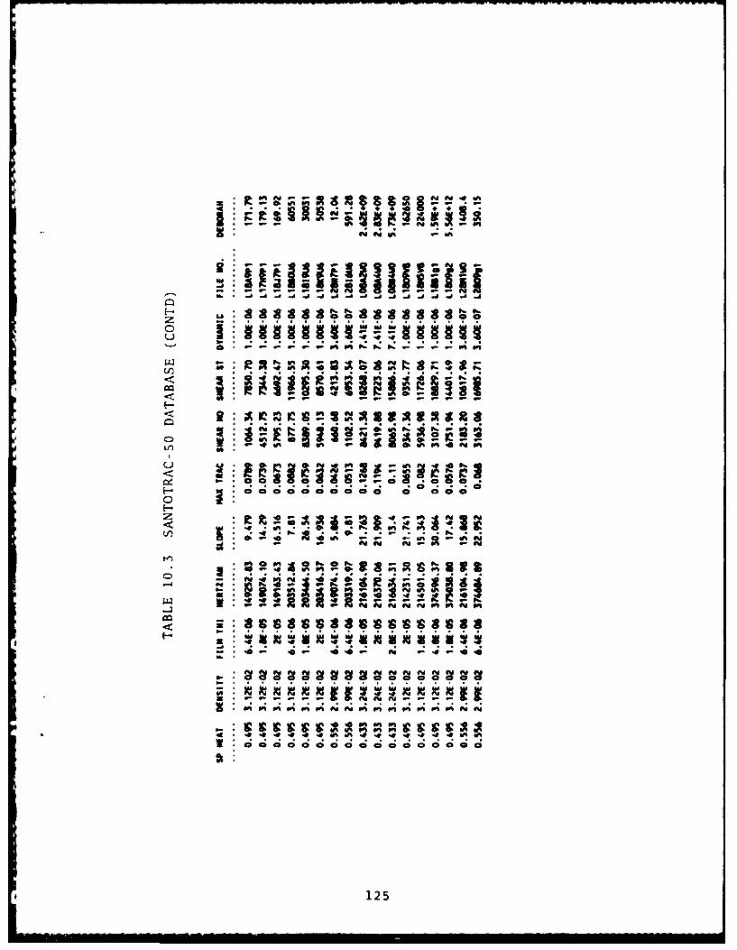
.- . .O O . .- .J
P; 0 FZ IN. o
oo
* o oo o a e on
oo
44, * --
: o1~~ 40S E --.w . . . . .- .- .. . F.. t
a D 4 4 0 4 2 N ; C;
125

C3 C3 a D a C3 a a a 0 a0 a a a a a2 a o
- - - -
WuUA
4A I, ft9' ry Nw Nt N N N N. NbP f N N N N N
M M Mu ONM mu mu Mu MIbbm~m ~ u m mu 0m m m m
U *~~ - -bbb~ Y~ - - - - - - - -
mb C3 D0 P -10 0 1
N ' ' .NN ee in
*O - Yb b b- - 4 01 y V ~ b
Yb- VIA A do wta
-i z a z" aNU~4 z z 3 It z zz z
012
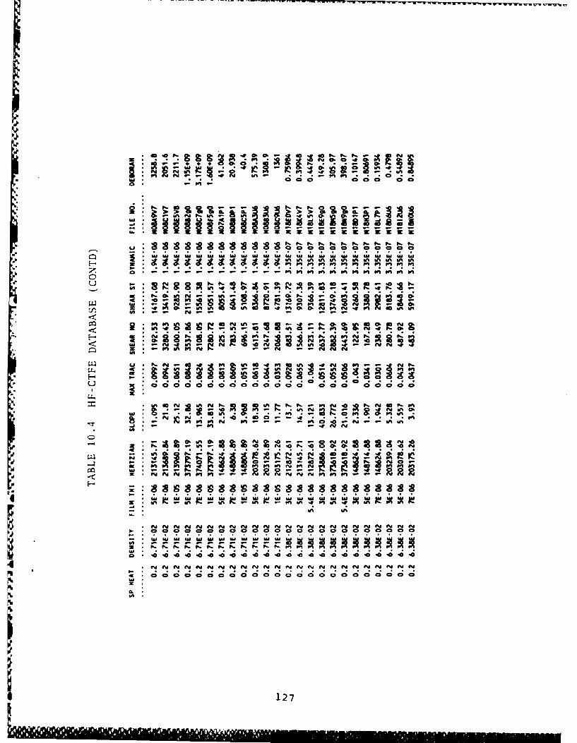
0: Ca
V, V, 6, ir % W% 4A in 61% b% V
u N0B N-, k0 '0 0 0 N B0: W! .0* n 0 - -
A .gBiN ;!
LLIr 0, NN n 044E 0 m QB U-4B~ I0t It- a t-
04o A op
on ct.
r. 4 N S a
ey -. an W% 0 0N BUon
W% O- -0 le 44 40 1110P,
No It 4* C3 2!-N gotg
AA rB,1
eI * N y on N n N n Nt Ny Nv M N N% N - -
- l It vi~ Miwi i V iwiitiWW I MwW
N ~ ~ ~ ~ ~ V LA NNNNNoue % yf yf I 4t yf yf 4ey. Vr uf yf1? 1 , 4 3.0 ' ,C
*i N N N N N N N Ni NNNNNNN nNN4............ ... .. .. .
127
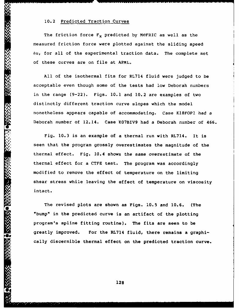
10.2 Predicted Traction Curves
The friction force Fx predicted by MCFRIC as well as the
measured friction force were plotted against the sliding speed
Au, for all of the experimental traction data. The complete set
of these curves are on file at AFML.
All of the isothermal fits for RL714 fluid were judged to be
acceptable even though some of the tests had low Deborah numbers
in the range (9-22). Figs. 10.1 and 10.2 are examples of two
distinctly different traction curve slopes which the model
nonetheless appears capable of accommodating. Case KI8FOPI had a
Deborah number of 12.14. Case K07BIV9 had a Deborah number of 466.
Fig. 10.3 is an example of a thermal run with RL714. It is
seen that the program grossly overestimates the magnitude of the
thermal effect. Fig. 10.4 shows the same overestimate of the
thermal effect for a CTFE test. The program was accordingly
modified to remove the effect of temperature on the limiting
shear stress while leaving the effect of temperature on viscosity
intact.
The revised plots are shown as Figs. 10.5 and 10.6. (The
"bump" in the predicted curve is an artifact of the plotting
program's spline fitting routine). The fits are seen to be
greatly improved. For the RL714 fluid, there remains a graphi-
cally discernible thermal effect on the predicted traction curve.
1284 '
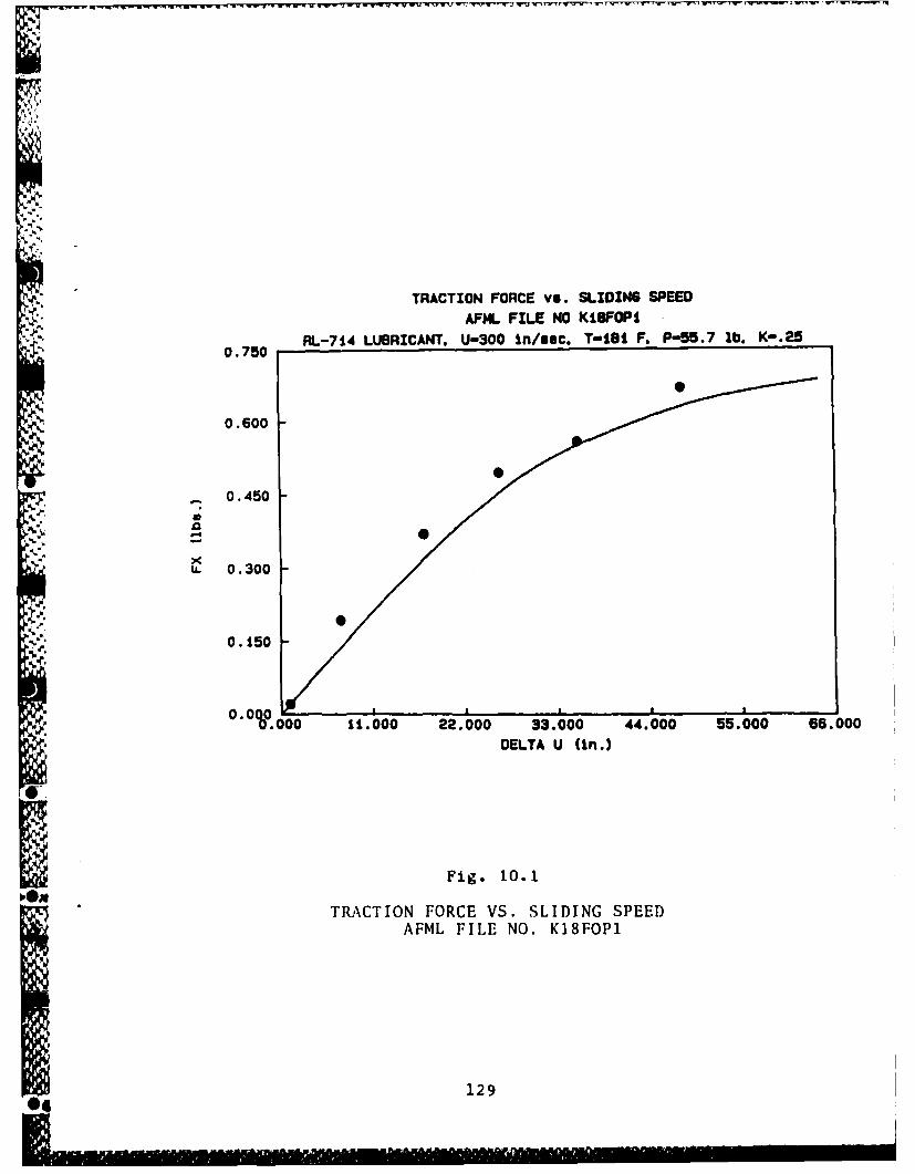
TRACTION FORCE vs. SLIDING SPEED
AFNL FILE NO KISFOPI
RL-714 LUBRICANT. U-300 In/sec. T-AIS F. P-55.7 lb. K-.250.750
0.600
. 0.450
0 -0.300
0.150
0-".OOO0 11.000 22.000 33.000 44. 000 55.000 66.000
DELTA U (in.)
Fig. 10.1
TRACTION FORCE VS. SLIDING SPEEDAFML FILE NO. K18FOP1
129
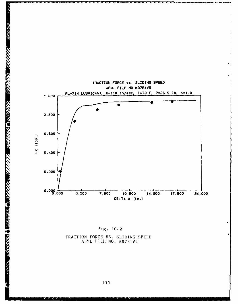
TRACTION FORCE vs. SLIDING SPEED
AFML FILE NO KO7BIV9
RL-714 LUBRICANT. U-11O in/sec. T-78 F. P-26.9 lb. K-1.01.000
0e
0.800
J 0.600
4 .0
ax
L. 0.400
0.200
0.000 - .0.000 3.500 7.000 10.500 14.000 17.500 21.000
DELTA U (In.)
Fig. 10. 2
TRACTION FORCE VS. SLIDING SPEEDAFML FILE NO. K07BIV9
130
TRACTON FORCE vs. SLIDING SPEED
AFML FILE NO K1009V7
0.500 RL-714 LUBRICANT. U-600 in/sec. T-182 F. P-26.0 lb. K-1.0
0.500
0.300
0.200
- 0.300
0.100
000 20.000 40.000 60.000 60.000 100.000 120.000
DELTA U (in.)
Fig. 10. 3
TRACTION FORCE VS. SLIDING. SPEEDAFML FILE NO. K1809V7
131

DO
TRACTION FORCE vs. SLIDING SPEEDAFML FILE NO MISBNGG
8.000 HF-CTFE LUBRICANT. U-748 lrt/uc. T-103 F. P-140. 1. K-1. 0
6.400
4.8900
xI. 3.200
V 1.600
00 7.000 14.000 21.000 28.000 35.000 42.000
DELTA U (in.)
Fig. 10.4
TRACTION FORCE VS. SLIDING SPEED)AFNIL FILE NO. N118N9GO
132
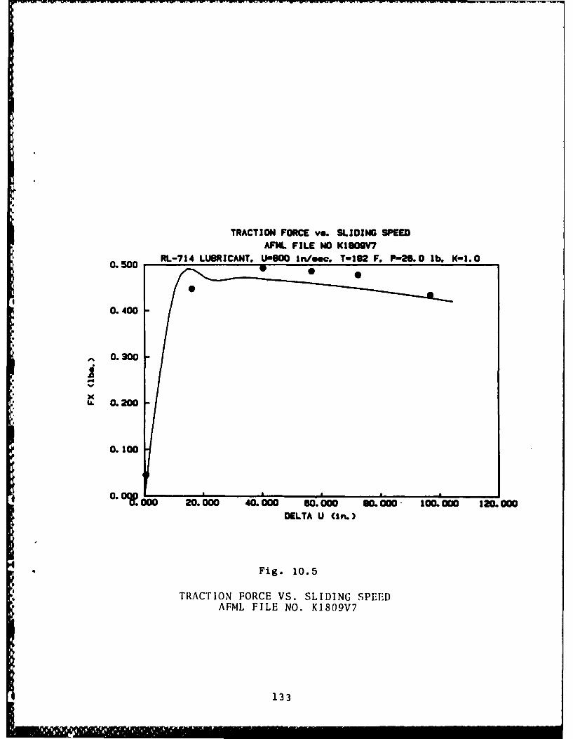
TRACTION FORCE vs. SLIDING SPEED
AFML FILE NO K1909V7RL-714 LUBRICANT. U,900 In/mo. T-1S2 F. P-26.O lb. K-1.O0. 500 _
0.400
0. 300
II* ii.0.200
0. 100
0 2. &W 40.0 O. 000 G.o. o - 10000 120.000DELTA U (In.)
Fig. 10.5
TRACTION FORCE VS. SLIDING SPEEDAFML FILE NO. K1809V7
133
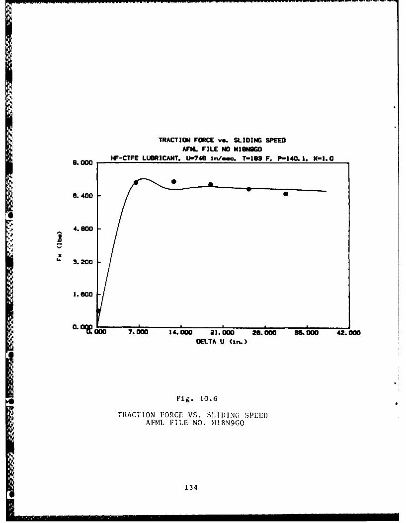
TRACTION FORCE vs. SLIDING SPEEDAFNL FILE NO NISNG
_._0 HF-CTFELUBRICANT.U-749In/se._T-1lSSF._P-140._1._K-I. 0
&.400
4.800
xLL 3.200
1.600
L OO00 7.0050 14.00 23.000 28. &00 35.6M0 42.000DELTA U (in.)
* Fig. 10.6
TRACTION FORCE VS. SIDING SPEED)ABIL FILE NO. M1SN9GO
134

The experimental traction data for Santotrac did not exhibit
a decrease at high sliding speeds suggestive of a thermal effect.
Figs. 10.7 and 10.8 show, respectively, the experimental and
isothermally predicted results for case L28H7Pl which had the
lowest calculated Deborah number among the Santotrac tests
(12.04), and for case L08B4WO which had the largest Deborah
number value. Both fits are judged to be acceptable.
Fig. 10.9 shows a plot of the results of a thermal run
applied to Santotrac case L17H9P1 (Deborah No. = 179) using the
original version of the program. Fig. 10.10 shows a thermal run
with the modified program. The program output does show a tem-
perature decrease at high sliding, but it is too small to be
graphically perceptible.
10.3 Viscoplastic Regime
The most serious discrepancy between predicted traction and
experimental traction force values occurred in the 9 CTFE tests
for which the Deborah number was less than unity.
4 These tests were all performed at a nominal temperature of
180OF at which the pressure viscosity index is 7.14E-5 in2/lb.
Fig. 10.11 shows the isothermally predicted and experimental data
for File No. Ml8EOV7 for which the Deborah number value is 0.76.
The predicted curve appears to have too low an initial slope and
fails to become asymptotic over the range of sliding speeds
represented by the experimental data.
135
- ..- ~ ,*
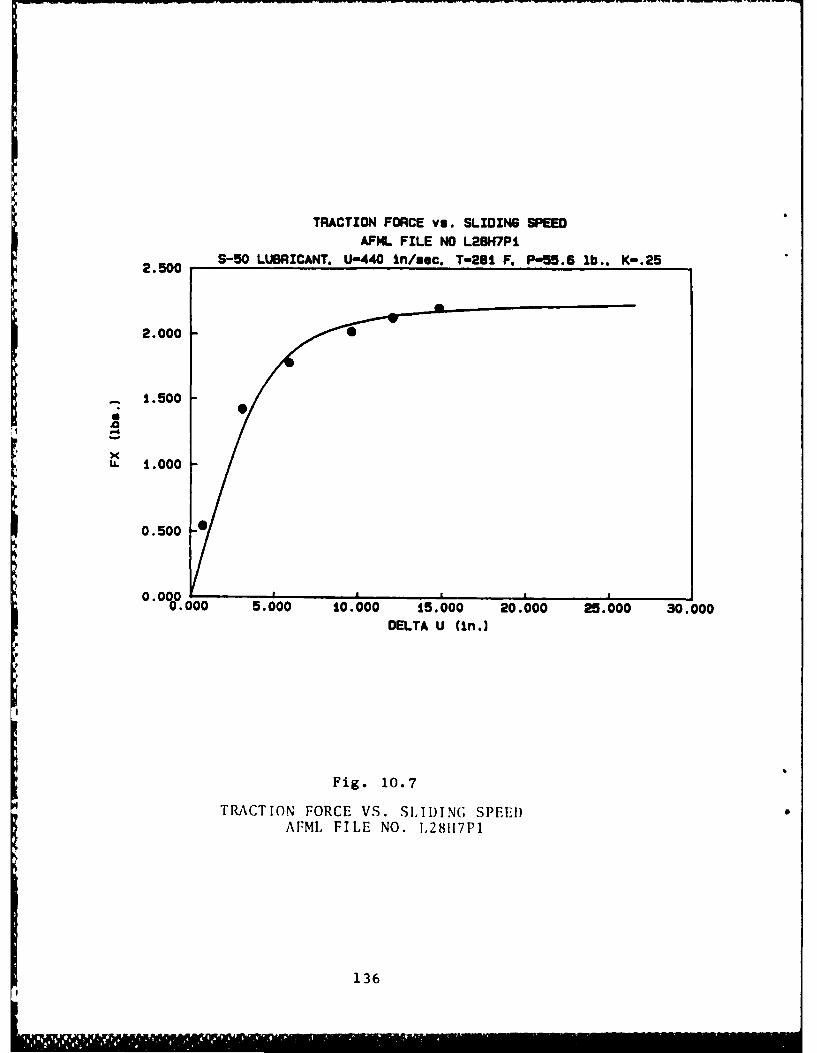
TRACTION FORCE vs. SLIDING SPEED
2500 AFML FILE NO L2BH7PI
2.500 S-50 LUBRICANT. U-440 In/sec. T-2181 F. P-55.6 lb.. K-.25
- 1.500
IL 1.000
0.500
O' OO 5.000 10.000 15.000 20.000 25.000O 30.000DELTA U (in.)
Fig. 10.7
TRACTION FORCE VS. SLIDING SPEED)AFML FILE NO. 1,28117P1
136
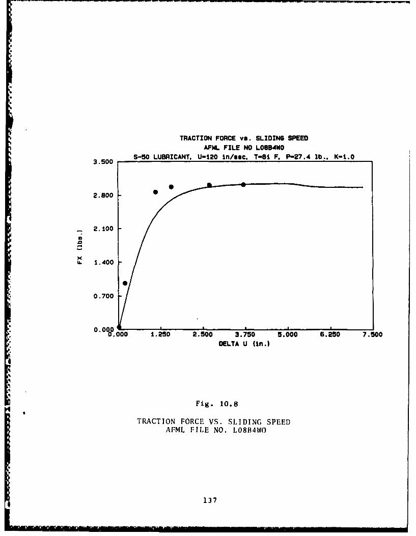
TRACTION FORCE vs. SLIDING SPEEDAFML FILE NO L08B4WO
3.500 9-50 LUBRICANT. U-120 In/sec. T-81 F. P-27.4 lb.. K-1.0
3.500
2.800
2.100
U. 1.400
0.700
0. 000__0000 1.250 2.500 3.750 5.000 6.250i 7.500
* DELTA U (in.)
Fig. 10. 8
TRACTION FORCE VS. SLIDING SPEEDAFML FILE NO. L08B41V0
137

TRACTION FORCE vs. SLIDING SPEED
AFML FILE NO L17H9PI
5.000 5-50 LUBRICANT. U-450 In/sec. T-179 F. P-55.6 lb.. K-.25
4.000 0
3.000
A.2.000
1.000
0V.000 31333 6.887 10.000 13.333 16.657 20.000
DELTA U (in.)
* Fig. 10.9
TRAcTrION FORCE VS. SLIDING SPEEDV AFML FILE NO. L17119Pl
138
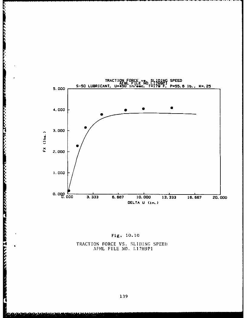
TRACT '0 810EEv~b E SPEED
500 S-5D LUBRICANT. U-4d in/sec. T-I~ P-55.6 lb.. K-.25
4.000 0
3.000
LL 2.000
5 1.000
0. W00 3.333 6.667 10.000W 13.333 16.667 20.0O0DDELTA U (in.)
Fig. 10. 10
TRACTION FORCE VS. SLID)ING SPEED)AFNIL FILE NO. 1,17H9P1
139
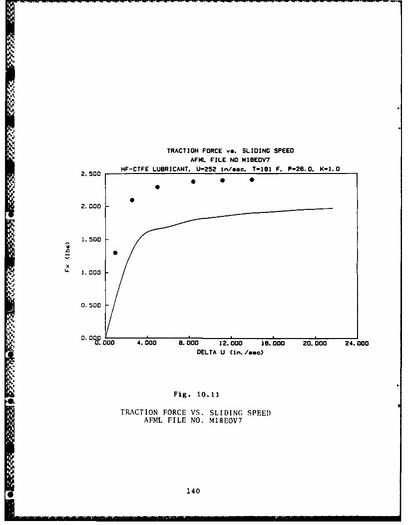
TRACTION FORCE vs. SLIDING SPEEDAFML FILE NO MI9EOV7
2.500 HF-CTFE LUBRICANT. U-252 in/sec. T-181 F. P-26.0. K-1.0
2.000
2 .000
0.500
Fi. 1.000
0.CTO 500 S.SIIN PE
0.000E O.M8EV
* 0.000 4.000 8.~~100 1.00 1.0 0 0 4 0
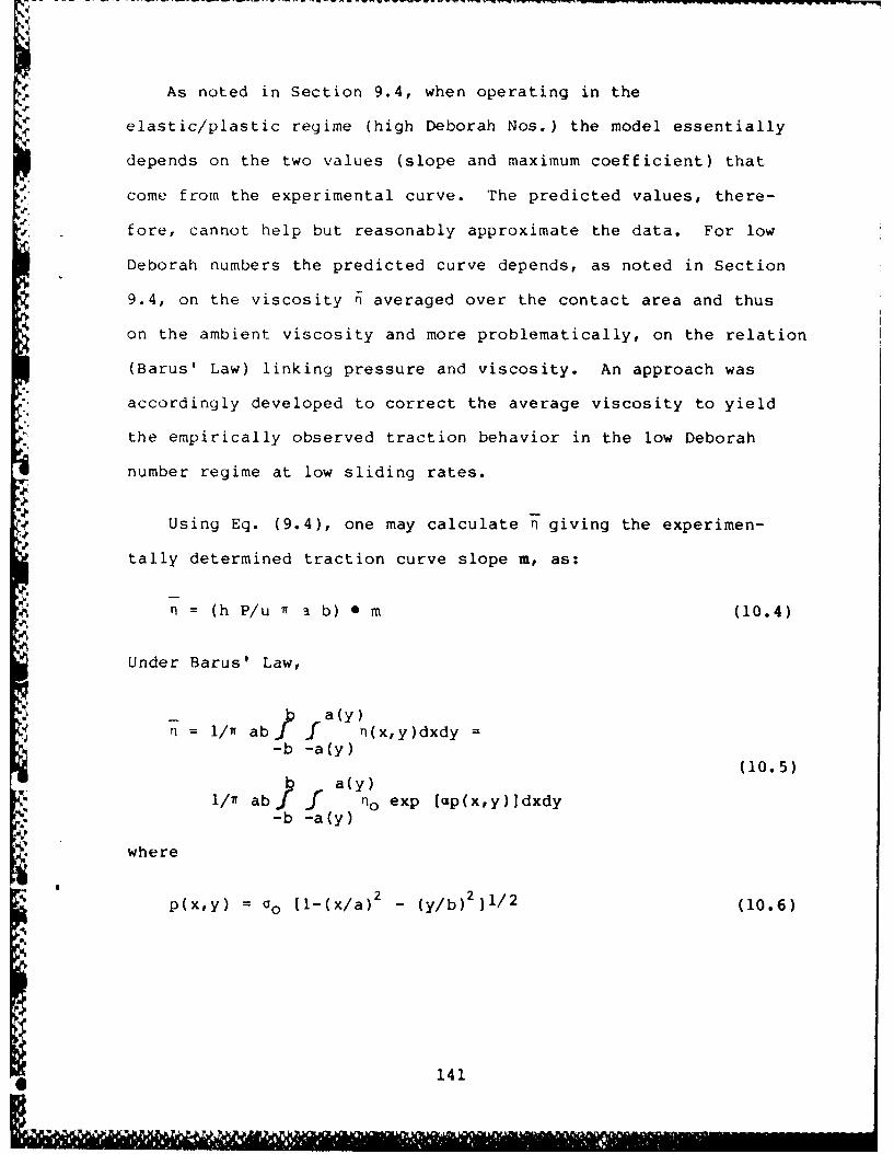
As noted in Section 9.4, when operating in the
elastic/plastic regime (high Deborah Nos.) the model essentially
depends on the two values (slope and maximum coefficient) that
come from the experimental curve. The predicted values, there-
fore, cannot help but reasonably approximate the data. For low
Deborah numbers the predicted curve depends, as noted in Section
9.4, on the viscosity n averaged over the contact area and thus
*on the ambient viscosity and more problematically, on the relation
(Barus' Law) linking pressure and viscosity. An approach was
* accordingly developed to correct the average viscosity to yield
.* the empirically observed traction behavior in the low Deborah
number regime at low sliding rates.
Using Eq. (9.4), one may calculate n giving the experimen-
tally determined traction curve slope m, as:
n (h P/u w a b) 0 m (10.4)
Under Barus' Law,
= 1/1 ab -b - (x,y)dxdy=-b -a (y)
(10.5)b a(y)
1/7 ab f -f no exp (ap(x,y)]dxdy-b -a(y)
where
U2
p(x,y) = o o [1-(x/a) 2 - (y/b) 2 j/2 (10.6)
141
- 3....--

and
a(y) = a[l-(y/b)2 1/2 (10.7)
Transforming to
Y = y/b
and X = x/a
gives n = no Il/ (10.8)
where
l+[l-Y2 ]1/2
Ii = II(Co)= SS exp [aol-X2 -y2] 1/2dxdy (10.9)
-i [I-Y 2 ]1/2
For u = 0, 11(o) is the area of the unit circle, i.e. w, so
that n in this case reduces to
n = no
I1 was evaluated by numerical integration over the range of aco
from 1.0 to 100. The relationship between Il and coo was
approximated as follows:
XnI 1 = a + b (aaO ) + c(a O )2 (10.10)
The values of a, b and c found by least squares over four subin-
tervals from ao = 1 to 50, are summarized below:
142
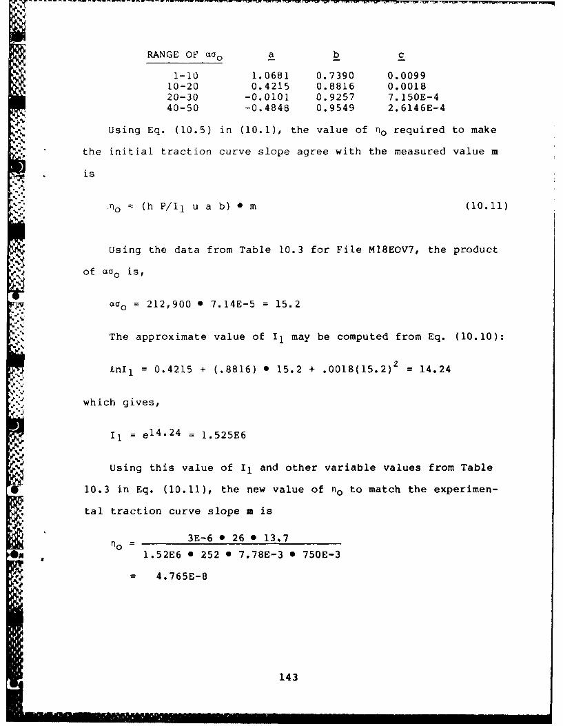
RANGE OF oo a b C
1-10 1.0681 0.7390 0.009910-20 0.4215 0.8816 0.001820-30 -0.0101 0.9257 7.150E-440-50 -0.4848 0.9549 2.6146E-4
Using Eq. (10.5) in (10.1), the value of no required to make
the initial traction curve slope agree with the measured value m
* . is
C..
no = (h P/I1 u a b) * m (10.11)
Using the data from Table 10.3 for File M18EOV7, the product
of U 0o is,
C oO = 212,900 * 7.14E-5 = 15.2'.
<C. The approximate value of I1 may be computed from Eq. (10.10):
XnI1 = 0.4215 + (.8816) * 15.2 + .0018(15.2)2 = 14.24
which gives,
I1 = e1 4 .2 4 = 1.525E6
Using this value of Il and other variable values from Table
S- 10.3 in Eq. (10.11), the new value of no to match the experimen-
tal traction curve slope m is
no 3E-6 0 26 0 13.7
1.52E6 0 252 * 7.78E-3 0 750E-3
= 4.765E-8
143
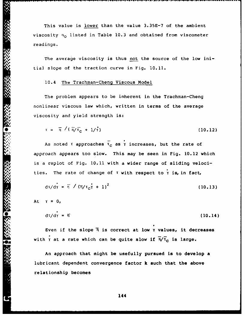
This value is lower than the value 3.35E-7 of the ambient
viscosity no listed in Table 10.3 and obtained from viscometer
readings.
The average viscosity is thus not the source of the low ini-
tial slope of the traction curve in Fig. 10.11.
10.4 The Trachman-Cheng Viscous Model
The problem appears to be inherent in the Trachman-Cheng
nonlinear viscous law which, written in terms of the average
pviscosity and yield strength is:p.
T = / c + i/) (10.12)
As noted T approaches Tc as ¥ increases, but the rate of
approach appears too slow. This may be seen in Fig. 10.12 which
is a replot of Fig. 10.11 with a wider range of sliding veloci-
ties. The rate of change of t with respect to y is, in fact,
dE/dy = n / (-/Tc; + 1)2 (10.13)
At Y = 0,.i
* dT/dy = T (10.14)
Even if the slope -n is correct at low r values, it decreases
with ; at a rate which can be quite slow if n/i[c is large.
An approach that might be usefully pursued is to develop a
lubricant dependent convergence factor k such that the above
relationship becomes
144
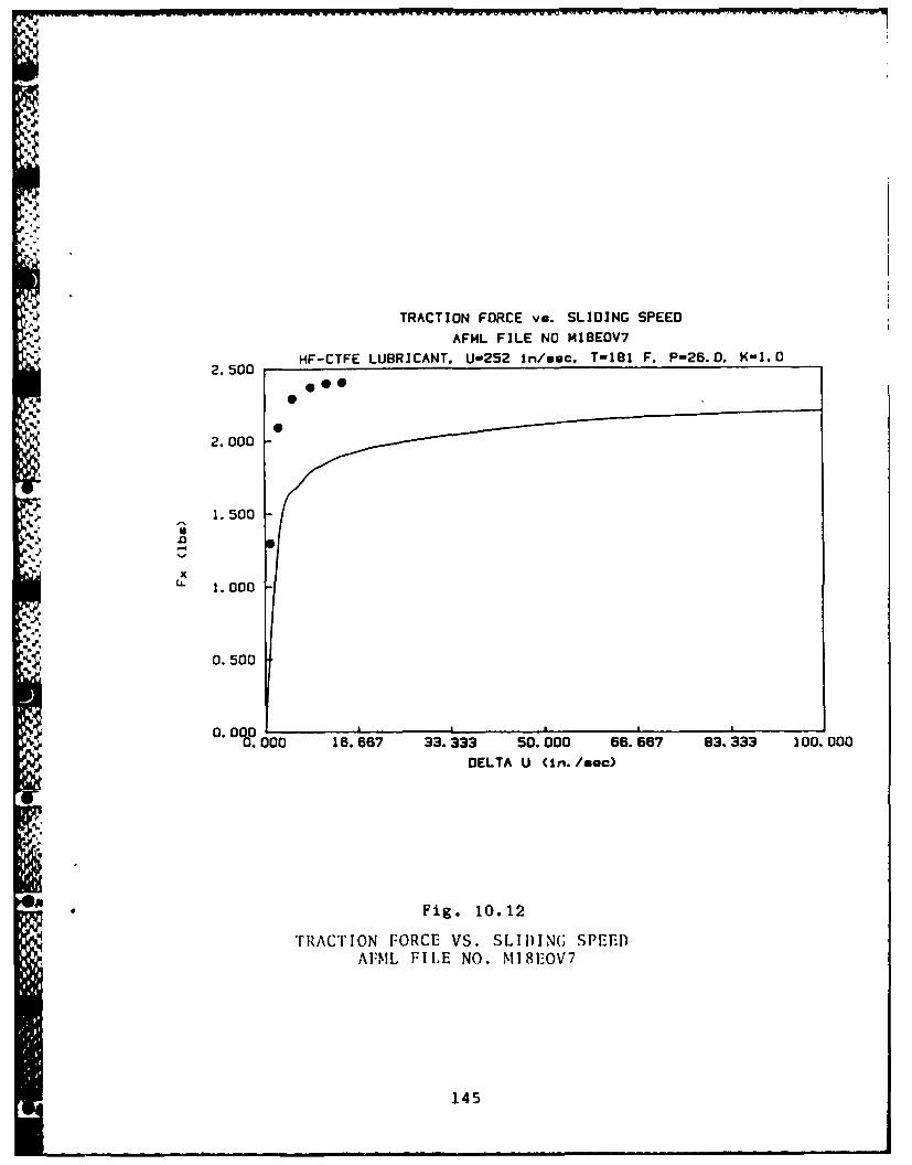
TRACTION FORCE vo. SLIDING SPEED
AFML FILE NO MIBEOV7
HF-CTFE LUBRICANT. U-252 In/oec. T-11 F. P-26.0. K-1.0
o00
2. 5Q02. 000
1.500
1.004- 1.0O00
0. 500
0. 000 16. 667 33. 333 50. 000 66. 667 83. 333 100. 000
DELTA U (In./sec)
* Fig. 10.12
TRACTION FORCE VS. SLIDING SPEEDAFML FILE NO. N118EOV7
145
T, n/(n/ c + 1/ki) (10.15)
This value could "tune" the approach to the asymptotic
limiting stress Tc . Such a factor would be analogous to the
parameter T0 which appears in the Ree-Eyring model and determines
where nonlinearity sets in. It is recommended that this or com-
parable alternative approaches for modulating the rate of con-
vergence to T-c in the viscoplastic regime be examined in future
work.
10.5 Alternative Approach to Speeding Convergence Rate
*A different approach that does not involve a fundamental
change in the rheological model was considered for restraining
the viscoplastically predicted traction curve from becoming asymp-
totic too slowly with strain rate.
As discussed, the empirically measured traction curve has a
slope m at low Au and approaches an asymptote at which T = T c .
Projecting the straight line portion of the traction curve it can
* be deduced that the traction curve becomes horizontal at a slide-
to-roll ratio Au/u in the vicinity of:
hu/u = IPmax/m (10.16)
The shear rate at this point is thus
= Au/h = U Mmax/mh (10.17)
146

It is reasonable to require that t given by the T-C relation
has risen to nearly the value T -Tc at this shear rate. Taking
I = 0.991c and using Eq. (10.17) in (10.12) gives
0.99 1c = n/( 0/Tc + mh/u Pmax) (10.18)
Solving for n gives,
= 99Tc m h/u Pmax (10.19)
Using Pmax = Fx/P where
Fx = T c 0 ab (10.20)
and P may be written
P = 2/3 ao 0 'ab (10.21)
so that
Pmax = 1.5 T c/Go (10.22)
giving
n = 99 mhoo /(u * 1.5) (10.23)
It is recalled that the G value input to the program is
deduced from the empirically measured value of a under the
assumption that the linear portion of the traction curve is due
to elastic deformation. From Eq. (9.6), a may be re-expressed as
m = 8 a2 bG/3Ph = 4 aG/v h co (10.24)
147
Using (10.24) in (10.19) results in
n = (8099)/3 0 (aG/a u) (10.25)
Using Eq. 10.5, this gives the modified ambient viscosity
value n0 of
no = 264 aG/u II*1
Using the values from Table 10.3, this calculates out to,
1= 264 0 7.78E-3 0 883.5 = 4.74E-6 (10.26)252 0 1.52E6
Using this value of no in the traction calculation (but not
in the film thickness calculation) results in the excellent fit
shown in Fig. 10.13. A recomputation in this manner has been
incorporated into McFRIC and is used wherever the Deborah number
falls below unity.
The nature of this "fix" is revealed by Eq. (10.25) which may
be written as
nu/aG = 84
This, except for the difference in computation of n, is the
Deborah number. The fix, therefore, amounts to changing low
Deborah numbers to large Deborah numbers, thereby causing the
traction curve slope at low slip to be determined by the elastic
modulus.
148

TRACTION FORCE vs. SLIDING SPEED
AFML FILE NO MI6EOV7
2.500 HF-CTFE LUBRICANT. U-252 in/sec. T-181 F. P-26.. K-1.0
2. 080
1.560
xLL 1.040
0. 520
0.00ffc.00 4. 000 63.000 12.D 000 16.00 20.000) 24. 000
DELTA U (in./sec)
Fig. 10. 13
TRACTION FORCE VS. SLIDING SPEED)AFML FILE NO. 1\I8EOV7
149
Whether this is correct cannot be judged with the present
data. It is necessary, following Johnson and Roberts [14] to
measure lateral force in the presence of spin to distinguish
elastic and viscous behavior. As it stands the program as
modified is capable of predicting the results of simple traction
tests for all three test oils.
10.6 Estimating G and Tc
McFRIC requires input data namely G and Tc, that must be
deduced from tractioii tests conducted at the contact conditions
of interest.
To overcome this, equations were fitted to the traction data
using stepwise linear regression in order to express the limiting
shear stress and shear modulus as functions of temperature T
(°F), maximum Hertz pressure p (psi), aspect ratio (AR), and
rolling velocity U (in/sec).
The coefficients in the relationships thus determined are
tabled below for each of the three oils.
150
i J "i: * P .. .. I * I
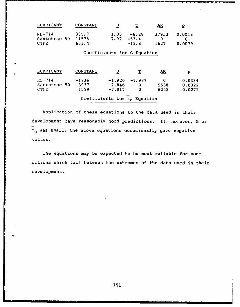
LUBRICANT CONSTANT U T AR, R
RL-714 365.7 1.05 -6.28 379.3 0.0018Santotrac 50 11576 7.97 -53.4 0 0CTFE 651.4 -12.8 1627 0.0079
Coefficients for G Equation
LUBRICANT CONSTANT U T AR P
RL-714 -1736 -1.926 -7.987 0 0.0334Santotrac 50 3937 -7.846 0 5538 0.0322CTFE 1599 -7.017 0 6258 0.0272
Coefficients for 'c Equation
Application of these equations to the data used in their
development gave reasonably good predictions. If, hovever, G or
Ic was small, the above equations occasionally gave negative
values.
The equations may be expected to be most reliable for con-
ditions which fall between the extremes of the data used in their
development.
15
151

REFERENCES
1. Hamrock, B. J. and Dowson, D., "Isothermal ElastohydrodynamicLubrication of Point Contacts, Part III - Fully FloodedResults," J. Lub. Technology, Vol. 99, No. 2, pp. 264-276(April 1977).
2. Murch, L. E. and Wilson, W.R.D., "A ThermalElastohydrodynamics Inlet Zone Analysis," Trans. ASME, J.Lub. Tech., 97F, No. 2, p. 272 (1975).
3. Hertz, H., "On the Contact of Rigid Elastic Solids and onHardness," Miscellaneous Papers, MacMillan & Co., London, pp.163-183 (1896).
4. Tevaarwerk, J. L. and Johnson, K. L., "The Influence of FluidRheology on the Performance of Traction Drives, ASME J. Lub.Tech., Vol. 101, p. 266 (1979).
5. Bair, S. and Winer, W. 0., "Some Observations in HighPressure Rheology of Lubricants," J. Lub. Tech., Vol. 104,No. 3, pp. 357-364 (1982).
6. Greenwood, J. A. and Williamson, J., "Contact of TwoNominally Flat Rough Surfaces," Proc. Roy. Soc. London, Ser.A, 295, pp. 300-319 (1966).
7. McCool, J. I., "Relating Profile Instrument Measurements tothe Functional Performance of Rough Surfaces," ASME J. ofTribology, Vol. 109, No. 1, pp. 264-270 (1987).
0 8. McCool, J. I., "Comparison of Models for the Contact of RoughSurfaces," Wear, 107, pp. 37-60 (1986).
9. Longuet-Higgins, M. S., "The Statistical Analysis of aRandom, Moving Surface," Philos. Trans. Royal Soc., Ser. A,249, pp. 321-387 (1957).
10. Bush, A. W., Gibson, R. D. and Keogh, G., "The Limit ofElastic Deformation in the Contact of Rough Surfaces," Mec.Res. Commun., 3, pp. 169-174 (1976).
11. Sayles, R. S. and Thomas, T. R., "Thermal Conductance of aRough Elastic Contact," Appl. Energy, 2, pp 249-267 (1976).
12. Wedeven, L. D. and Cusano, C., "Elastohydrodynamic Contacts -
Effects of Dents and Grooves on Traction and Local FilmThickness," NASA Technical Paper 2175, June 1983.
13. McCool, J. I., "Traction Model Development," Air ForceMaterials Lab, Technical Report No. AFWAL-TR-85-4142, (May1986).
152
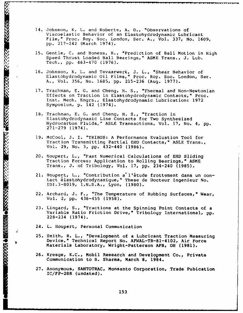
14. Johnson, K. L. and Roberts, A. D., "Observations ofViscoelastic Behavior of an Elastohydrodynamic LubricantFilm," Proc. Roy. Soc. London, Ser. A., Vol. 337, No. 1609,pp. 217-242 (March 1974).
15. Gentle, C. and Boness, R., "Prediction of Ball Motion in HighSpeed Thrust Loaded Ball Bearings," ASME Trans., J. Lub.Tech., pp. 463-470 (1976).
16. Johnson, K. L. and Tevaarwerk, J. L., "Shear Behavior ofElastohydrodynamic Oil Films," Proc. Roy. Soc. London, Ser.A., Vol. 356, No. 1685, pp. 215-236 (Aug. 1977).
17. Trachman, E. G. and Cheng, H. S., "Thermal and Non-NewtonianEffects on Traction in Elastohydrodynamic Contacts," Proc.Inst. Mech. Engrs., Elastohydrodynamic Lubrication: 1972Symposium, p. 142 (1974).
18. Trachman, E. G. and Cheng, H. S., "Traction inElastohydrodynamic Line Contacts for Two SynthesizedHydrocarbon Fluids," ASLE Transactions, Vol. 17, No. 4, pp.271-279 (1974).
19. McCool, J. I. "TRIBOS: A Performance Evaluation Tool forTraction Transmitting Partial EHD Contacts," ASLE Trans.,Vol. 29, No. 3, pp. 432-440 (1986).
20. Houpert, L., "Fast Numerical Calculations of EHD SlidingTraction Forces; Application to Rolling Bearings," ASMETrans., J. of Tribology, Vol. 17, pp. 234-240 (1985).
21. Houpert, L., "Contribution a'l'etude frottement dans un con-tact elastohydrodynamique," These de Docteur Ingenieur No.IDI.3-8019, I.N.S.A., Lyon, (1980).
22. Archard, J. F., "The Temperature of Rubbing Surfaces," Wear,Vol. 2, pp. 438-455 (1958).
23. Lingard, S., "Tractions at the Spinning Point Contacts of aVariable Ratio Friction Drive," Tribology International, pp.228-234 (1974).
24. L. Houpert, Personal Communication
25. Smith, R. L., "Development of a Lubricant Traction Measuring* Device," Technical Report No. AFWAL-TR-81-4102, Air Force
Materials Laboratory, Wright-Patterson AFB, OH (1981).
26. Kresge, K.C., Mobil Research and Development Co., PrivateCommunication to S. Sharma, March 8, 1984.
27. Anonymous, SANTOTRAC, Monsanto Corporation, Trade PubicationIC/FP-28R (undated).
153
- - i ' I IA
28. Sharma, S. K., "Ambient Properties of CTFE," unpublishedmemorandum, (1984).
29. Jones, W., Johnson, R., Winer, W. 0., and Sanborn, D.,"Pressure Viscosity Measurements for Several Lubricants to5.5xi0 8 Newtons Per Square Meter (8x10 4 psi) and 149*C(300 0F)," ASLE Trans., Vol. 18, No. 4, pp. 249-262.
30. Sharma, S. K., "Traction Data/Ambient Properties," PersonalCommunication, (June 5, 1986).
P.
ph
III
*154 U.S. GPO 5qS-OS

im
9w V :