'~' ~;~~"",,":~"'4''''''''-'':;'''''-' ,. ,."""' ........"'~,~.",,.~, ·'.i·'~.', ,_.,,, "~ ".", ro

', •• , ...., • ...;' .,~-,"-;;-...

"' A Theoretical Analysis of Plant Host- IPathogen Interactions in a Gene-for-Gene ISystem I

Ronald John Czochor

Biomathematics Series No. 8 IInst. of Statistics Mimeo Series No. 1603

l.~__~.".,-c>c,: ...-:",,,,,,,...,,,,,-._·...~<, ...,.... ...._ ... ,,.,,..·,...,... n·',-,,''''''_-'~'"O"''''''''''~_'''__'''V'-'''''~'"'''__'''''''"'~''''-'',","".~.

ABSTRACT

CZOCHOR, RONALD JOHN. A Theoretical Analysis of Plant Host-Pathogen

Interactions in a Gene-for-Gene System. (Under the direction of H. R.

VAN DER VAART.)

The explanatory value of the concepts of selection against

unnecessary virulence in the pathogen and selection against unnecessary

resistance in the host was investigated using a mathematical model first

proposed by Leonard (1977). The model was changed from a simultaneous

pair of difference equations to a sequential pair of difference equations

in order to better· reflect the way the frequencies change in nature. A

linear analysis was conducted on both pairs and the simultaneous model was

shown to have a locally unstable internal equilibrium point while the

analysis of the sequential model produced inconclusive results. Numerical

simulation of the sequential model produced inward spirals which led

credence to the suspicion that stable limit cycles or a stable equilibrium

point existed. The analysis of the higher order terms of the Taylor

expansion required the development of a technique for discrete time

difference equations that was ana1agous to that developed by Poincare

(1885) for continuous time differential equations. For parameter values

in which stability could be expected biologically, the internal equilibrium

point was found to be locally stable.

Also discussed was the potential application of a multiple niche

model to the study of gene frequency change in the pathogen on a multiline

crop. The model was analyzed and the internal equilibrium point was

determined to be stable in some regions of the parameter space. The fact

that a multiline crop could produce such a polymorphism in the pathogen

said little about the effectiveness of this strategy in preventing an

epidemic, since the pathogen population could be increasing at a high

rate while still maintaining a polymorphism.

A model was developed to study the increase of the pathogen

population on either the multiline or single variety crop. The change

in the number of lesions of each pathogen race was modeled with the

amount of uninfected leaf area considered as a, limiting factor. The

relative site of a lesion in each host-pathogen combination was a crucial

factor in describing host resistance. The ease with which parameters

could be measured was emphasized and a preliminary comparison was made

between rotation of two host varieties and simultaneous planting of the

two varieties. In this simplistic comparison, the simultaneous planting

(multiline crop) appeared to be less effective, except when the reproductive

rate or initial size of the pathogen population was very low.

TABLE OF CONTENTS

1. INTRODUCTION.

2. LITERATURE REVIEW

3. A MODEL FOR COEVOLUTION IN GENE-FOR-GENE SYSTEMS ••

PAGE

1

6

13

v

4. THE CENTER-FOCUS PROBLEM. • • • • • • • • • • • • 37

5. A POTENTIAL MULTILINE MODEL FOR GENE FREQUENCY.

6. A MULTILINE MODEL FOR PATHOGEN POPULATION GROWTH•.

53

61

7. CONCLUSION. 83

8. APPENDICES •• 88

8.l.

8.2.

8.3.

8.4.

8.5.

8.6.

8.7.

8.8.

Derivation of equation (3.1).

Derivation and proof of equation (3.2) ••

Calculation of eigenvalues of the Jacobian of(3.2) at the trivial singular points (0,0), (0,1),(1,0), (1,1) .

Calculation of eigenvalues of the Jacobian of(3.5) evaluated at the internal equilibriumpoint (n*, p*) • • • • • • • • • • • • • • • •

Calculation of eigenvalues of the Jacobian of(3.5) evaluated at the triva1 points (0,0), (0,1),(1,0), (1,1). • • • • • • • •••••••

Poincare's method applied to Leonard's model ••

Expressions in terms of the original parametersfor the coefficients of the Taylor seriesexpansion . . . . . . . . . . . . . . .

Proof that A1245 is a 5x4 matrix of rank 4 • • • .

89

90

92

97

99

102

112112

113

-"

.t

9. LITERATURE CITED. . • . . 116

1. INTRODUCTION

One of the methods used in the control of plant disease is the

deployment of resistant cu1tivars. With modern agricultural practices,

this usually means that large areas are planted with one variety of

one species of crop. In many instances, this genetic uniformity

presents an opportunity for a genetically malleable pathogen population

to overcome the resistance and create disease of epidemic proportions.

However, in some instances, this so-called breakdown of resistance

does not occur. It would then be advantageous to plant crops such

that the resistance does not break down or at least such that the time

until breakdown is prolonged.

Before we look further into this issue, we must realize that

there are two types of disease resistance. According to Van derP1ank

(1963), vertical resistance (VR) occurs "when a variety is resistant

to some races of the pathogen" and horizontal resistance (HR) occurs

"when the resistance is evenly spread against all races of the pathogen".

Unfortunately, these two terms have caused quite a stir in the plant

pathology literature, so that now they have many different meanings.

Van der Plank (1963) actually started the problem when he stated in

his discussion of the effect of resistance on an epidemic that VR would

have the effect of reducing the initial amount of disease and that HR

would normally have the effect of reducing the rate of disease increase.

This, however, caused some to consider these effects as the actual

definitions of the terms. Then in his next book Van derPlank (1968)

decided that since races of the pathogen could differ in aggressive­

ness, the presence of HR could not be easily determined unless

2

he interpreted the definitions as follows: "vertical resistance ~

implies a differential interaction between. varieties (of host) and

races (of pathogen)" and "in horizontal resistance there is no

differential interaction". This enabled VR to be determined through

analysis of variance or through a ranking procedure to test for

significant differences between rankings of pathogen aggressiveness

compared to pathogen rankings on a known horizontally resistant

variety. However, VR no longer implied differential interaction

between varieties and races; in his new book, Van der Plank (1975)

stated that VR was actually equivalent to this interaction.

Again in 1975, he discussed vertical resistance and horizontal

resistance, but this time he used a theory put forth by Flor (1955).

Working with the host plant flax, Linum usitatissimum, and its rust

causing pathogen, Melampsora lini; Florwas able to show a one-to-one

matching in which a specific allele in the flax confers resistance to

a specific allele in the rust. This he called the gene-for-gene

theory which has since been shown to be valid for many other plant

disease systems (Flor, 1971). Van der Plank said that VR would be

resistance for which a gene-for-gene hypothesis is conceivable and

that HR would be resistance for which it would not be possible.

Problems with the analysis of variance test for VR and with

inconsistencies with the original definitions were brought out by

Robinson (1976), Parlevliet and Zadoks (1977), and Nelson (1978). These

eventually caused Van der Plank (1978) to further dilute the dichotomy

to VR with specificity, VR without specificity, and HR. This was quite

different from the original definition in 1N'hich VR ;vas such resistance eas is specific for some races only.

3

Thus there is more than one type of resistance and there is

disagreement on the definitions of the different types of resistance.

It will then be necessary to limit our discussion to one of the

hypothesized types of resistance, and so, we shall confine our 'study

in the following chapters to vertical resistance with specificity in

a theoretical gene-for-gene system. Of ultimate interest is the

genetic relationship between the different varieties of host plant and

the different races of one species of pathogen and hence all external

influences in the form of inputs to and outputs from this subsystem will

not be considered.

In a gene-for-gene system, Van der Plank theorized that there must

be two types of selection going on. He called them directional selection,

by which he meant selection favoring the resistance gene in the host or

selection favoring the virulence gene in the pathogen; and stabilizing

selection, by which he meant selection against unnecessary resistance

or virulence. Since the term stablizing selection has been used

differently in the genetic literature, we shall use the term selection

against unnecessary resistance or against unnecessary virulence. Such

selective forces had to be in effect since gene-far-gene systems would

never have been discovered if selection inevitably favored resistance in

the host population and virulence in the pathogen population. A gene

for resistance cannot be recognized except in comparison with its

allele for susceptibility, and genes for resistance will not be recognized

if the corresponding gene for avirulence is missing from the pathogen

population. Therefore, Van der Plank argued that vertical resistance

would not have been found unless genes for avirulence were sometimes

selectively favored over genes for virulence.

4

There have been numerous arguments against this concept of ~

selection against unnecessary resistance. These have been summarized

by Crill (1977) and Nelson (1972, 1973), but neither Nelson nor Crill

dispute the logic behind the concept. In Chapter 3, we shall look at

an explanatory model representing this concept and analyze it to

determine whether the observed polymorphic populations of host and

pathogen can be explained by this type of selection. A problem arising

in the analysis of the model necessitates the development of a new

analytic technique which is described in C:hapter 4.

The implementation of vertical resistance in an agricultural system

of just one variety will prOVide almost total resistance to disease for

a while until a virulent race of the pathogen develops. Then a calamitous

breakdown of the resistance occurs due to directional selection in

favor of the virulent pathogen race. Hence we have the boom and bust

cycle so prevalent with use of vertically resistance varieties in a

monoculture.

This presents an especially difficult problem since the creation of

suitable, resistance varieties is a time consuming process. A method

for circumventing this cycle has been proposed by Jensen (1952) and

Borlaug (1953) in the form of multiline cropping practices, in which

many varieties of the same crop species would be randomly planted to­

gether. It is thought that this would promote a polymorphic pathogen

population with subsequent low levels of disease comparable to what is

observed in natural co-evolutionary systems. A possible model for this

type of agricultural practice along with an analysis of its stability

will be presented in Chapter 5.

The ultimate question to be addressed through mathematical

modeling of this type of system is whether multiline cropping

practices or development of the varieties separately in a sequence

of pure line cu1tivars would be more effective in preserving the

longevity, in terms of usefulness, of the resistant varieties. A

model to address this question will be developed in Chapter 6.

There have been a number -of models proposed to describe the

coevolution of the host and its pathogen in a gene-for-gene system

as well as models for describing multiline systems. In the next

chapter, which parallels Leonard and Czochor (1980) some of these

models will be presented. This review will present a historical

background for the studies undertaken in this dissertation.

5

6

2. LITERATURE REVIEW

The models that have been proposed to describe the genetic

interactions between populations of plants and their pathogens can

be classifiedin one of two categories. In the first section of this

chapter, a review of the models of gene-for-gene interactions, their

assumptions, and conclusions will be conducted. Later, models that

have been developed to describe multiline cropping systems will be

discussed.

Mode (1958) was one of the first to use a mathematical model

to analyze genetic interactions between populations of plants and

their pathogens in gene-for-gene relationships. He based his model

on a system with two genes for resistance that are alleles at a single

locus andtw.o corresponding genes for virulence that occur at indepen­

dent loci where they are distinguished from alleles for avirulence.

He assumed that the fitness of a host in a particular host-pathogen

combination varies inversely with the fitness of the pathogen, and

that in genetically mixed populations, the fitness of a particular

pathogen genotype is determined by weighting its fitness in each

combination with a host genotype by the frequency of that host

genotype. The model also assumed continuous change in genotype fre­

quencies instead of the discrete change necessitated by the assumption

of distinct generations. His analysis of this model showed that a host­

pathogen system could reach a stable equilibrium provided that certain

conditions were met. These conditions werE~ presented in mathematical

terms, so it was not easily apparent what the biological basis for the

stable equilibrium might be. In fact, the example that Mode used to

7

illustrate a stable equilibrium had no fitness values greater than

zero, which is biologically absurd. Also Mode's model could not account

for the persistence of genes for susceptibility.

In his second model, Mode (1960) studied the change in the

frequencies of the various cultivars and races rather than gene

frequencies as in his previous model. This model was just a special

case of the model Mode (1961) presented the following year. In these

models, as in his previous model, he assumed continuous increase of the

various populations in order to simplify the analysis. He did, however,

recognize that in fact, the generations of the host at least were

discrete. Since the assumption of continuous increase usually allows

greater chance for stability than increase in discrete generations

(see May, 1973), this assumption could very well lead to a conclusion

of stability for an equilibrium point that actually is not stable.

Other assumptions were also the same as in his first model.

In his general model, Mode (1961) considered four classes of

stationary states: (i) when population number in both the host and

pathogen populations is constant; (ii) when population number in the

host population is constant, but that in the pathogen population is

variable; (iii) when population number in the host population is

variable, but in the pathogen population is constant; and (iv) when

population number in both the host and the pathogen is variable. If

selection coefficients in this model are allowed to vary, a stable

equilibrium can occur in all four of the above classes. However, if

selection coefficients are constant, a stable equilibrium can occur in

classes (ii), (iii), and (iv), but not in class (i). Class (i) is just

Mode's (1960) second model. Although Mode gives the conditions under

8

which stability is expected, it is not apparent what they are

in terms of biological constraints. He also suggested that in

agriculture, a host population consisting of a mixture of cultivars.

would be superior to a population consisting of a single cultivar

only if the mixture tended to slow down the selection of new pathogenic

races. This type of result will be addressed in Chapter 6.

In analyzing his models, Mode found that the frequencies of

pathogen races at equilibrium are determined by the fitness of host

cultivars and that the frequencies of host cultivars at equilibrium

are determined by the fitness of pathogen races. These features were

also found by Jayakar (1970) and Leonard (1977) in subsequent host­

pathogen models.

Jayakar (1970) developed a model principally with the interaction

of bacteria and bacteriaphage in mind, but which is applicable to most

host-pathogen interactions. He labeled the probability that a given

host individual is infected if it is susceptible, as x_. He then

started with a simple model, assuming that once a host is infected by a

pathogen, it dies and the pathogen reproduces so that an average of

n offspring are produced. He also assumed that if the host cannot be

infected because of resistance, then the host individual reproduces

and the pathogen dies. The model is for a single locus for resistance

in the host and a single locus for virulence in the pathogen. The A

genotype ofthe host is susceptible to both the B and the b genotype

of the pathogen. The a genotype of the host is resistant to the

B (avirulent) genotype and susceptible to the b (virulent) genotype

of the pathogen. The frequencies of A and a genotypes in the

9

host population, respectively, are P1 and 1-P1; and the frequencies

of Band b in the pathogen are Pz and 1-PZ' respectively.

Jayakar showed that this model will not produce a polymorphism,

since it is selecting only for the virulent pathogen genotype which

will eventually make the two host types effectively selectively neutral.

Next, Jayakar added the concept put forth by Van der Plank in the

study of plant epidemics of some other type of selection that could

balance with this directional selection in favor of the virulent

pathogen. In fact, he generalized his model to be able to incorporate

this type of selection by letting f be the inherent fitness of a

relative to A and g the inherent fitness of b relative to B. This

new model produced a non-trivial equilibrium point at P1 = g and

Pz = (l-x) (l-f)/xf, if the f and g were such that 0 < P1 < 1 and

o < Pz < 1. Jayakar found this internal equilibrium point to be

locally unstable, but his computer simulation showed that the trajecto­

ries actually cycled around in a closed ellipse that was probably

some type of limit cycle. He also pointed out that the addition of

mutation did not materially change this behavior. This model is very

muchfue same as a model that Leonard (1977) later developed specifically

to describe Van der Plank's concept of "stabilizing selection" in plant

disease. We shall see more of this in Chapter 3.

Once again in the plant pathogen literature, Person, et a1. (1976)

and Groth and Person (1977) considered a model for the effects of se­

lection on pathogen populations in gene-far-gene systems. The fitness

values assigned to the avirulent and virulent pathogen on the susceptible

host were land 1-sa , respectively, and the fitness values assigned to

the avirulent and virulent pathogen on the resistant host were I-Sa and

10

1, respectively. For the frequence of susceptible hosts equal to

m and the frequency of resistant host equal to n, they found that the

fitness of the virulent and avirulent genotypes would be equal when

n sA = m sa' Since sA is likely to be near one, the point of equal

fitness occurs when s = n/m •a

Leonard (1969) used essentially the same type of model, but the

fitness values assigned to the avirulent and virulent pathogen on the

susceptible host were 1 and l-s, respectively, and on the resistant

host the fitnesses were 0 and l-s , respectively. The point of equal

fintess for his model occurred when s = n.

The difference between the models of Person, et al. (1976, 1977)

and Leonard (1969) was mainly in the question of whether the virulent

pathogen genotype reproduces better on a resistant host than on a

susceptible host (Person's model) or equally well on both (Leonard's

model). In fact, there is a third choice that Nelson (1978, 1979)

suggested, that is that the virulent race 'would reproduce better on the

susceptible host than on the resistant host. One question that may be

answered through the analysis of a more ge:neral model is which of the

above ideas can better produce a stable polymorphism. Such a more

general model will be discussed in the next chapter.

The use of multiline varieties was suggested by Jensen (1952)

and Borlaug (1953) as a method of preventing the rapid shifts in

virulence in pathogen populations which have lead to epidemics in pure

line cultivars. Barlaug advocated the "clean crop approach" with its

goalof keeping the multiline free of disease by immediately replacing

any diseased variety. Browning and Frey (1969) advocated the "dirty crop eapproach" which is based on the assumptions that the multi-line varieties

...

11

can stabil~e the race structure of pathogen populations and that

this can be done with sufficient resistance in the host mixture to

prevent significant damage by the stabilized pathogen population. The

validity of these assumptions will be studied in Chapter 5 and through

a model developed in Chapter 6.

Kiyosawa (1972) compared theoretical calculations for the annual

increase of disease in cultivars grown either as a mixture or separately

in sequence with each cultivar being replaced when disease on it

reached a critical level. The usefulness of this approach depended

upon knowledge of the annual rates of disease increase in a multiline

Am ' and a pure line cultivar, A. He showed that the mixture will

have greater longevity than the sequence of pure line cultivars if

n A < A , where n is the number of cultivars. The estimation of thesem

rates from daily rates is possible, but when disease increase is limited

by available host tissu~ the problem becomes most complex. The simulation

model developed in Chapter 6 will address this problem.

Crill (1977) stated that in gene-for-gene systems, rotations of

pure line cultivars would be superior to multiline varieties. However,

he apparently based his conclusions on the dubious assumption that

selection against unncesssary genes for virulence in the pathogen

occurred only in the pure line system and not the multiline system.

Kiyosawa and Yabuki (1978) developed a model for gene frequency

in the pathogen population on a mixed host and concluded that the

equilibrium among the pathogen races could not occur without the

operation of selection against unnecessary virulence genes. An

analogous model with similar results will be discussed in Chapter 5.

12

Other models for multipline cropping systems proposed by ~

Groth (1976), Marshall and Prior (1978, 1979), Marshall and Weir

(1982), and Barret and Wolfe (1978) have all addressed the question"

of the multiline and the number of varieties needed in the multiline

to obtain a certain level of effectiveness.

13

3. A MODEL FOR COEVOLUTION IN GENE-FOR-GENE SYSTEMS.

In this chapter, we shall discuss a model developed by Leonard

(1977) that extended his earlier model (Leonard, 1969) to include the

interactions affecting selection pressures in the host population as

well as in the pathogen population. This model attempts to incorporate

Van der Plank's concept of selection against unnecessary resistance

and against unncecessary virulence into a gene frequency model of a

gene-for-gene host-pathogen system. It was hoped that incorporation

of these types of selection into such a model would be enough to

ensure genetic polymorphisms in both the host and'pathogen populations.

The observed coexistence of virulent and avirulent races of the pathogen

as well as of resistant and susceptible varieities of the host, would

then be explainable by Van der Plank's hypothesized selective forces.

Although Leonard developed the model, his analysis of" it was

limited to computer results for specific parametric values. In this

chapter and the next, we shall attempt a more general and more mathe­

matical analysis and by doing so in a fair amount of detail, we shall

hope to gain the ability to determine whether Van der Plank's hypothesis

can explain the observed polymorphisms. However, first we must describe

the model.

The model consists of two difference equations, one describing the

change ingene frequency at a locus with two possible alleles in a

diploid host and the other describing the change in gene frequency at

a locus with two possible alleles in a diploid pathogen. Difference

equations will be used instead of differential equations because the

host is assumed to have distinct generations separated by a part of the

14

instead of differential equations because the host is assumed to have

distinct generations separated by a part of the year which is not

part of the growing season (for most plants, this is winter). Also,

this part of the year requires that the pathogen have an overwintering

phase and hence, with reproduction once a year, the pathogen must also

have disctinct generations. In many disease systems, the pathogen

is known to have more than one generation per growing season. Since

some of these generations may be overlapping, a differential equation

for the gene frequency change may be called for; however, if we assume

no overlapping generations, difference equations may also be used for

the case of multiple pathogen generations per growing season.

The one locus, two allele case is,o~ course, the simplest one,

but its analysis is as complex as we would need for this hypothesized

selection regime. The model is a general explanatory model and as such

it make quite a few simplifying assumptions. It assumes random mating

in the host, and it assumes that the populations are large enough so

that random drift will not be a factor. Also, it is purely a selection

model and as such it assumes that both alleles in both the host and

pathogen are already present in the respective populations. Thus

mutation is not considered, but it could easily be worked into

the model, at least in any computer simulations. Also, since the model

is for gene frequencies and drift is not considered, the influence of

coevolution on population size is overlooked.

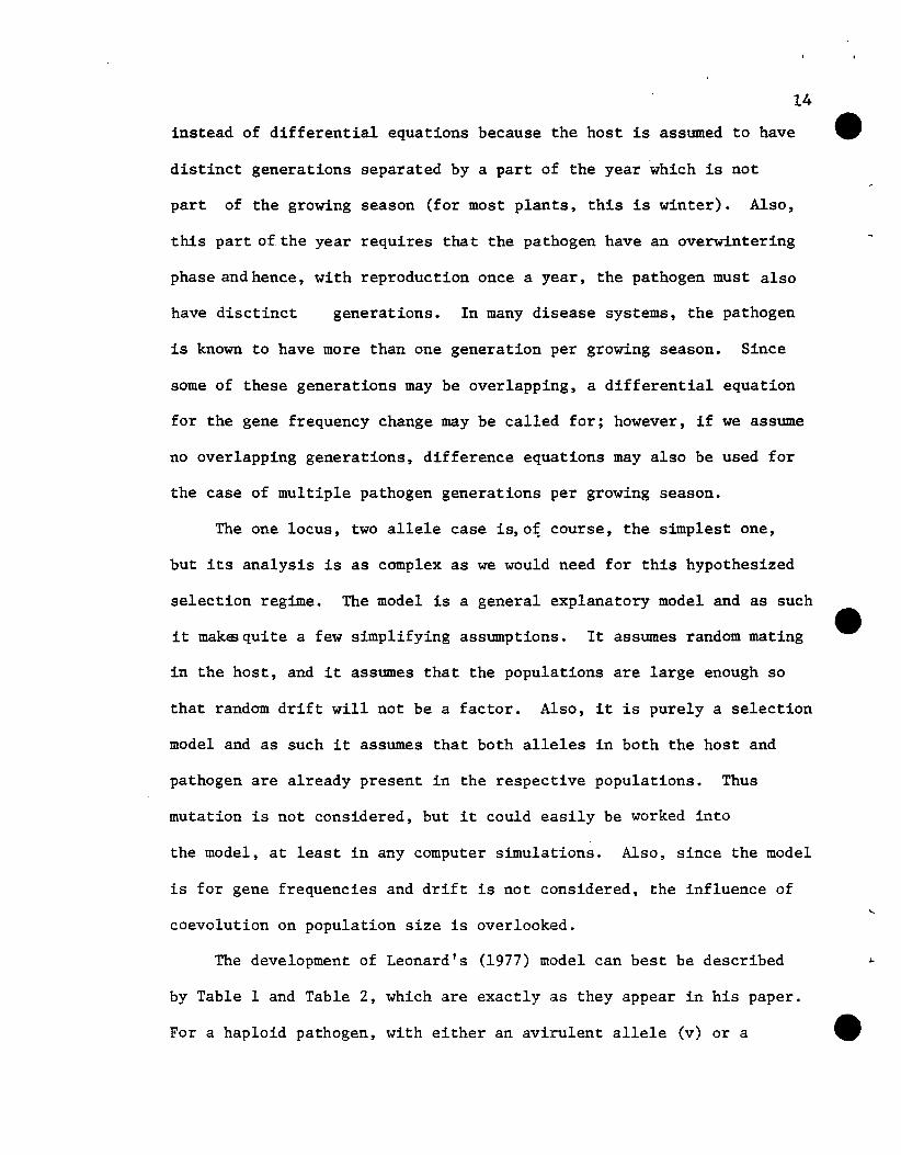
The development of Leonard's (1977) model can best be described

by Table 1 and Table 2, which are exactly as they appear in his paper.

For a haploid pathogen, with either an avirulent allele (v) or a

eh I,

e

Table 1. Relative Fitness of Pathogen Genotypes on Different Hosts.

e

Pathogen genotype andreaction resistant host(RR or Rr)

Relative fitnesses of pathogen genotypeson:

rr(susceptible) R_(resistant)

v(avirulent)

V(virulent)

1

l-k

l-t

l-k+a

Relative fitnesses of pathogen genotypes onmixed host population.

v

v

p = frequency of R

q = 1 - p

wv

\-lV

=

=

2 2q + (l-q ) (l-t)

qq(l-k) + (l-q2)(l-k+a)

....VI

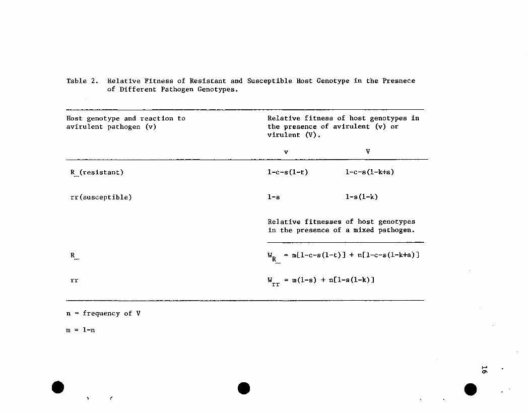
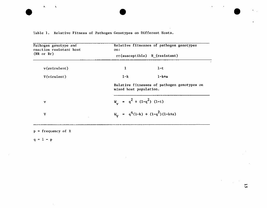
Table 2. Relative Fitness of Resistant and Susceptible Host Genotype in the Presneceof Different Pathogen Genotypes.

Host genotype and reaction toavirulent pathogen (v)

Relative fitness of host genotypes inthe presence of avirulent (v) orvirulent (V).

R_(resistant)

rr(susceptible)

v

l-c-s(l-t)

l-s

V

l-c-s(l-k+a)

l-s(l-k)

e

R

rr

n = frequency of V

m = l-n

r re

Relative fitnesses of host genotypesin the presence of a mixed pathogen.

W = m[l-c-s(l-t)] + n[l-c-s(l-k+a)]R

W = m(l-s) + n[l-s(l-k)]rr

e....0\

17

virulent allele (V), we can express the relative fitnesses of these

genotypes on the different host genotypes as in Table 1. By relative

fitness, we mean the proportionate contribution of offspring to the

next generation. Thus if the relative fitness of an avirulent

pathogen ona susceptible (rr) host is arbitrarily put equal to 1,

then the relative fitness of an avirulent pathogen on a resistant host

is l-t, where t is the effectiveness of resistance. Notice that we

are considering the resistant allele R to be completely dominant so that

both genotype RR and genotype Rr are resistant. Leonard estimated t

to be very close to 1 (between 0.98 and 1.00), since the avirulent

pathogen has relatively little or zero reproductive success if it is on

a resistant host.

The fitness of a virulent pathogen on the susceptible host will

be l-k, where k is the cost of virulence. This is where Van der

Plank's concept of selection against unnecessary virulence is incor­

porated. If k > 0 , then the avirulent pathogen will be more fit

than the virulent pathogen on the susceptible host where virulence

is unncessary. Leonard estimated that k would be in the range of 0.1

to 0.4. Notice that the virulent pathogen on the resistant host still

has this cost, k, but also involves another parameter a so that the

relative fitness of this virulent genotype on a resistant host has a

value of l-k+a. Depending on the value of the parameter a the model

for the pathogen fitness could be the same as a number of the models

or ideas that we have discussed in the previous chapter. For a = k ,

we would have a pathogen fitness array comparable to Person's (1976);

for a = 0 , it would be comparable to Leonard's (1969) model; for

a < a , it would be comparable to Nelson's (1978, 1979) ideas; and

18

for a > 0, we would have a fitness array comparable to that suggested ~

by Denward's (1967) data for late blight. Since analysis of the

stability of these models was not undertaken, a general analysis of

Leonard's model might help to discern the relative merits of the

above authors'positions.

The relative fitnesses of the pathogen genotype on a mixed host

population were then calculated, where q is the frequency of allele r

2and hence the frequency of the susceptible host is q and the frequency

of the resistant host is 1_q2 • The average over hosts of the relative

fitness of the pathogen in each combination will give us the relative

fitness on a mixed host population. Hence, the frequency of the virulent

gene,V, in generation T + 1, n(T+1), will be the frequency of the

virulent gene, V, in generation T times its fitness on the mixed host

population divided by the average fitness (Crow & Kimura, 1970, p.179 ).

Thus,

where Wv and Wv are the fitnesses on a mixed host population of the

virulent and avirulent pathogen genotypes, respectively.

Since the Wv and Wv are not functions of T, this is an autonomous

difference equation and can be written as

So we now have a recurrent equation for thl~ frequency of the virulent

pathogen gene in the next generation.

Next we look at the relative fitness of the resistant and

susceptible host genotype in the presence of the different pathogen

genotypes as displayed in Table 2. The fitness for the resistant host

19

in the presence of the avirulent pathogen is given by l-c-s(l-t).

In this instance,the parameter, c , is the cost of resistance and

like k for the pathogen, it incorporates Van der Plank's concept of

selection against unnecessary resistant into the model. Also, the

relative fitness of the resistant host in the presence of the avirulent

pathogen is lessened by s(l-t), the disease severity rating. The

parameter, s, concerns the suitability of the environment for disease

development and when multiplied by the relative fitness of the pathogen

in that combination of host variety and pathogen race, expresses the

fitness loss in the host due to disease.

Also, in Table 2, we have the relative fitness of the resistant

host in the presence of a virulent pathogen to be l-c-s(l-k+a) where

once again the fitness is reduced by the cost of resistance and by

the disease severity rating. For the susceptible host, the loss in

fitness is just due to disease severity; thus we have l-s for its

fitness in the presence of an avirulett pathogen and l-s(l-k) for its

fitness in the presence of a virulent pathogen.

The relative fitnesses of the host genotype in the presence of a

mixed pathogen population can then be calculated by averaging the

different fitnesses over the different pathogen genotypes. Then the

relative fitness of a resistant host genotype in the presence of a

mixed pathogen population will be designated WRRor WRr and the relative

fitness of a susceptible host genotype in the presence of a mixed

pathogen will be designated Wrr Now, the frequency of the dominant

resistant allele in generation T + 1, peT + 1), will be the

frequency of the homozygous resistant genotype times its fitness, plus

one-half of the frequency of the heterozygous resistant genotype

times its fitness divided by the average fitness (Crow and Kimura,

1970, p. 179).

20

ph+1) =WRR + peT) [l-p(T)]WRr

l-IRR

+ 2p(T)[1-p(T)]WR + [1-p(T)]2Wr rr

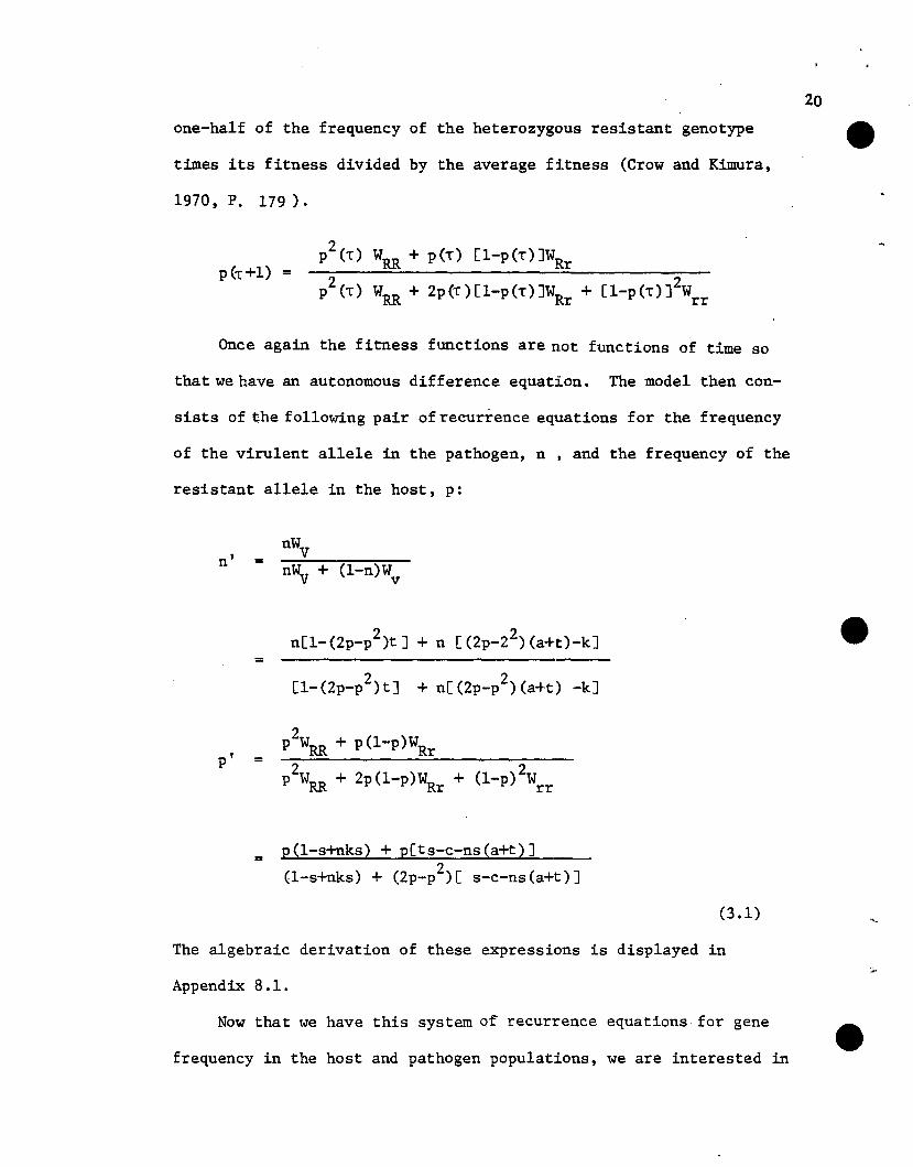
Once again the fitness functions are n.ot functions of time so

that we have an autonomous difference equation. The model then con-

sists of the following pair of recurrence equations for the frequency

of the virulent allele in the pathogen, n, and the frequency of the

resistant allele in the host, p:

n' =

=n[l-(2p-p2)t] + n [(2p_Z2) (a+t)-k]

[l-(Zp-pZ)t] + n[(2p-pZ)(a+t) -k]

p' =2P WRR + p(l-p)WRrZP WRR + Zp(l-p)WRr

= p(l-s+nks) + p[ts-c-ns(a+t)]Z(l-s+nks) + (Zp-p )[ s-c-ns(a+t)]

(3.1)

The algebraic derivation of these expressi.ons is displayed in

Appendix 8.1.

Now that we have this system of recurrence equations for gene

frequency in the host and pathogen populations, we are interested in

21

whether there is a stable internal equilibrium point or whether one

of the alleles in either or both the" host and "pathogen will become

fixed at some trivial equilibrium point. In order for this selection

regime to yield genotypically polymorphic populations of the host and

pathogen, it would be necessary to have a stable internal equilibrium

point or (at least) a- stable limit cycle about such an internal point.

This would prohibit the fixation of either allele in both the host

and the pathogen populations.

Thus we must determine whether the system (3.1) has an internal

equilibrium point and if it is stable. The point (n*, p*) will be an

equilibrium point of the system (3.1) if n*' = n* and p*' = p* •

We call (n*,p*) an internal equilibrium point if 0 < n* < 1 and

o < p* < 1 , and a trivial equilibrium point if both n* and p* are

equal to either 0 or 1. If either n* or p* (both not both) were

equal to either 0 or 1, the point (n*,p*) would not qualify as an

equilibrium point of (3.1). This, along with the existence of the

trivial equilibrium points (0,0), (1,0), (0,1), and (1,0) is obvious

from the equations of system (3.1). From the first equation of the system

(3.1), it can be seen that if p* is such that 2p* - p*2 = k/(a+t), then

n' = n and from equation two of system (3.1), it can be seen that if

n* = (ts-c)/s(a+t), then p' = p Thus (n*,p*), where n* = (ts-c)/

s(a+t) and 2p* - p*2 = k/(a+t) will be an internal equilibrium point

of (3.1) if 0 < n* < 1 and 0 < p* < 1 .

Leonard suggested the following for the ranges of the various

parameter values:

0.1 < k < 0.4

0.95 < t < LO

0.0 < a < 0.8

0.1 < s < 0.8

0.01 < c < 0.05

22

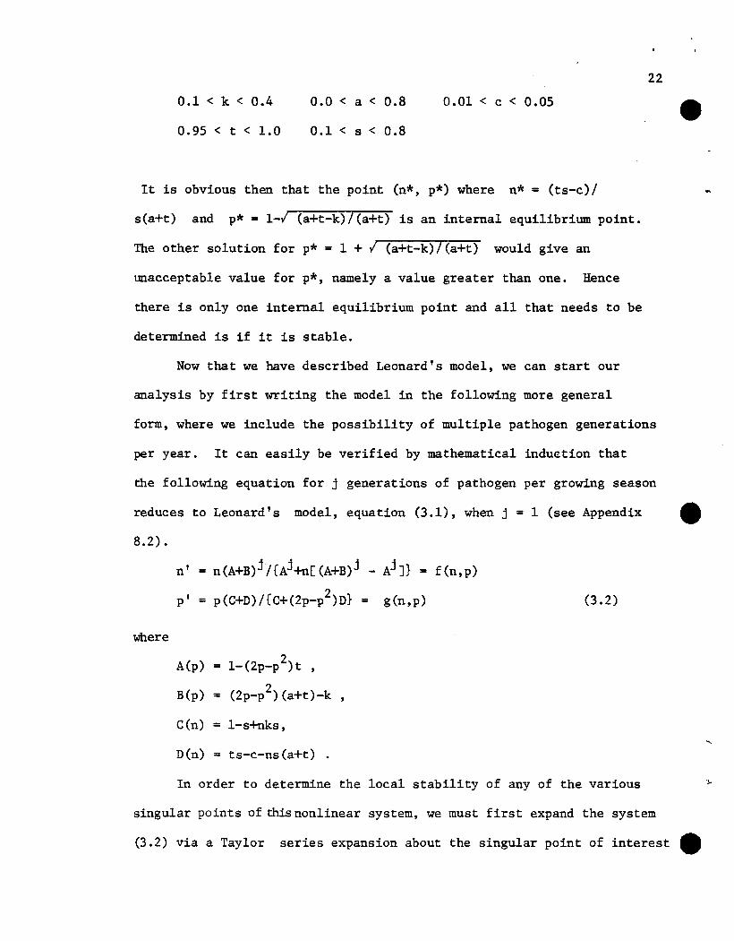
It is obvious then that the point (n*, p*) where n* = (ts-c)/

s(a+t) and p* = 1-1 (a+t-k) / (a+t) is an i.nternal equilibrium point.

The other solution for p* = 1 + I (a+t-k)/(a+t) would give an

unacceptable value for p*, namely a value greater than one. Hence

there is only one internal equilibrium point and all that needs to be

determined is if it is stable.

Now that we have described Leonard's model, we can start our

analysis by first writing the model in the following more general

form, where we include the possibility of multiple pathogen generations

per year. It can easily be verified by mathematical induction that

the following equation for j generations of pathogen per growing season

reduces to Leonard's model, equation (3.1), when j = 1 (see Appendix ~

8.2) .

where

n' = n(A+B)j/{Aj+n[ (A+B)j - Aj ]} = f (n,p)

p' = p(C+D)/{C+(2p-p2)D} = g(n,p)

A(p) 2= 1-(2p-p )t ,

B(p) = 2(2p-p ) (a+t)-k

C(n) = l-s+nks,

D(n) = ts-c-ns(a+t)

(3.2)

In order to determine the local stability of any of the various

singular points of this nonlinear system, we must first expand the system

(3.2) via a Taylor series expansion about the singular point of interest ~

23

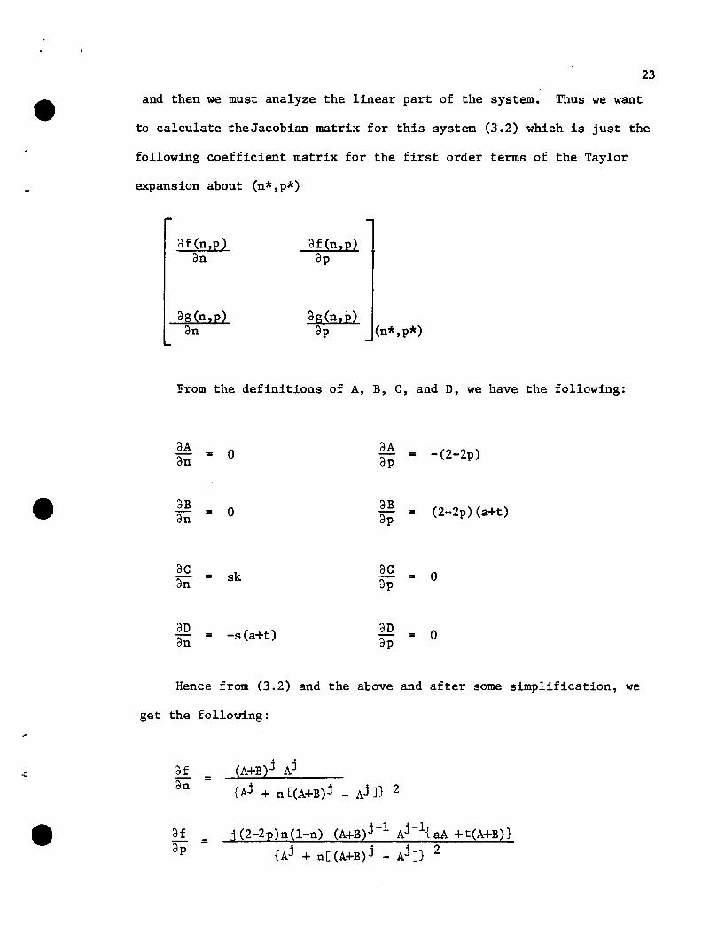
and then we must analyze the linear part of the system. Thus we want

to calculate the Jacobian matrix for this system (3.2) which is just the

following coefficient matrix for the first order terms of the Taylor

expansion about (n*,p*)

af (n,p)an

ag(n,p)ap (n*,p*)

From the definitions of A, B, C, and D, we have the following:

aA0

aA -(2-2p)an = =ap

aB0

aB (2-2p) (a+t)an = =ap

acan = sk

acap = 0

aDan = -s(a+t) aD

ap = 0

Hence from (3.2) and the above and after some simplification, we

get the following:

afan =

afap =

j (2-2p)n(l-n) (A+B)j-l Aj - 1{ aA +t(A+B)}

{Aj + n[ (A+B)j - Aj ]} 2

3 =dn

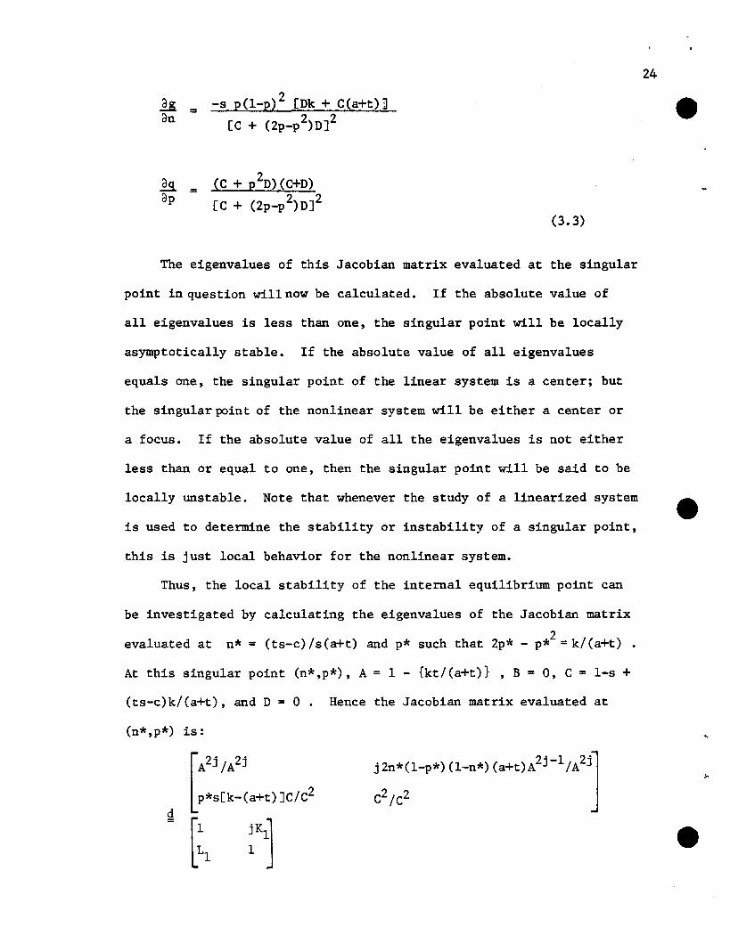
s =dP

-s p(1_p)2 [Dk + C(a+t)]

[C + (2p_p2)D]2

(C + p2D) (C+D)2 2[C + (2p-p )D]

(3.3)

24

The eigenvalues of this Jacobian matrix evaluated at the singular

point in question wi11now be calculated. If the absolute value of

all eigenvalues is less than one, the singular point will be locally

asymptotically stable. If the absolute value of all eigenvalues

equals one, the singular point of the linear system is a center; but

the singular point of the nonlinear system will be either a center or

a focus. If the absolute value of all the eigenvalues is not either

less than or equal to one, then the singular point will be said to be

locally unstable. Note that whenever the study of a linearized system

is used to determine the stability or instability of a singular point,

this is just local behavior for the nonlinear system.

Thus, the local stability of the internal equilibrium point can

be investigated by calculating the eigenvalues of the Jacobian matrix

evaluated at n* = (ts-c)/s(a+t) and p* such that 2p* - p*2=k/(a+t) •

At this singular point (n*,p*), A = 1 - {kt/(a+t)} , B = 0, C = 1-s +

(ts-c)k/(a+t), and D = o. Hence the Jacobian matrix evaluated at

(n*,p*) is:

j2n*(1-p*) (l-n*) (a+t)A2j-1/A2j]

c2/c2

e\

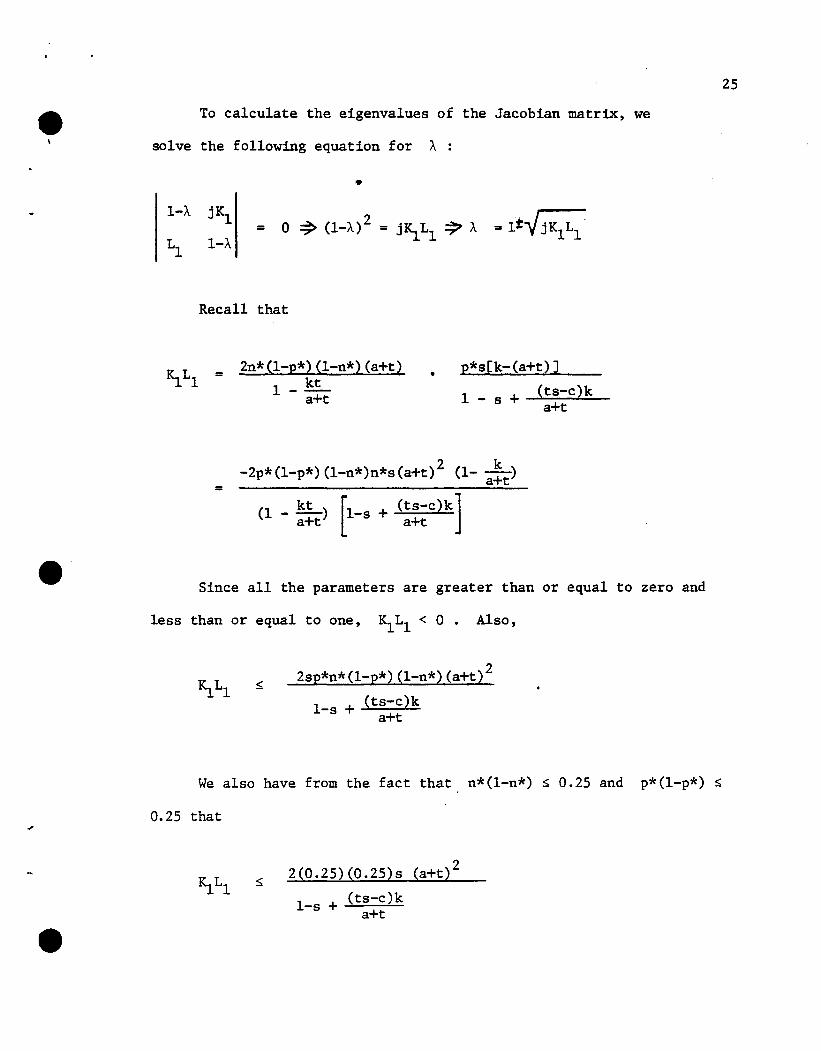
To calculate the eigenvalues of the Jacobian matrix, we

solve the following equation for A :

•

25

Recall that

2n*(1-p*) (l-n*) (a+t)1 _ kt

a+t

• p*s[k-(a+t)]

1 - s + (ts-c)ka+t

-2p*(1-p*)(1-n*)n*s(a+t)2 (1- ~)=

(1 _ kt ) [l-S + (ts-C)k]a+t a+t

Since all the parameters are greater than or equal to zero and

less than or equal to one, ~Ll < O. Also,

22sp*n*(1-p*) (l-n*) (a+t)

l-s + (ts-c)ka+t

We also have from the fact that n*(1-n*) $ 0.25 and p*(1-p*) $

0.25 that

2(0.25)(0.25)s (a+t)2

1-s + (ts-c)ka+t

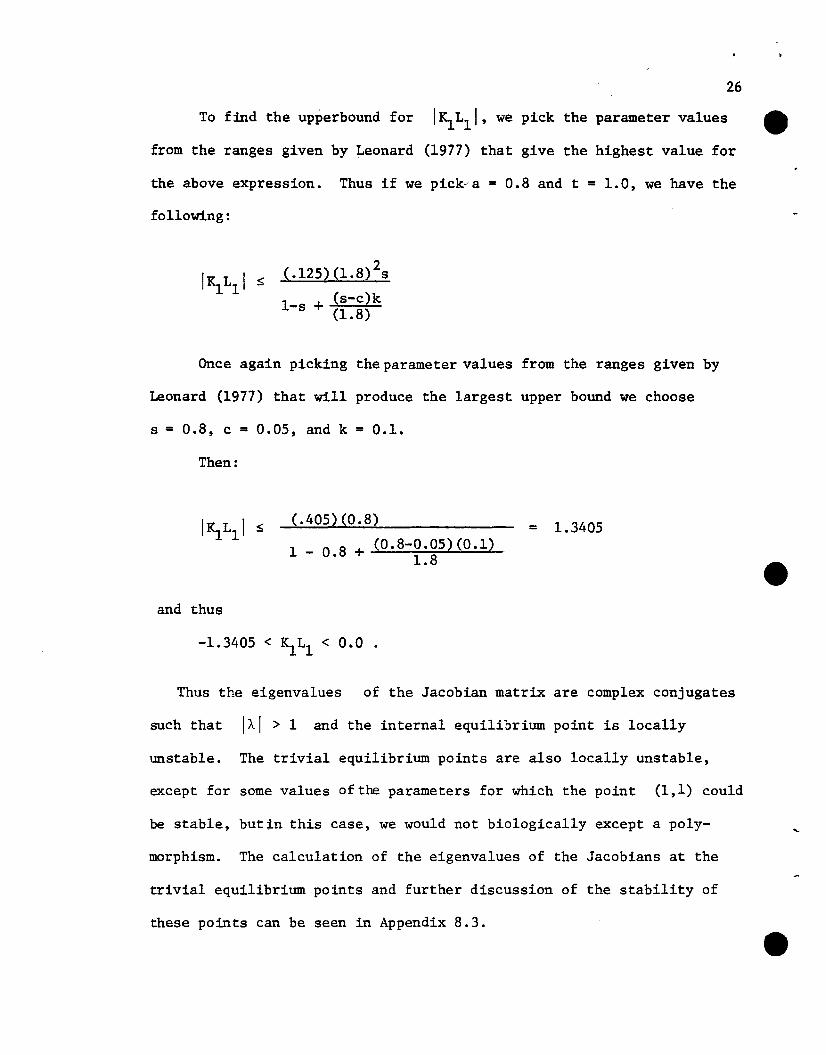
26

To find the upperbound for IIS.Lll, we pick the parameter values efrom the ranges given by Leonard (1977) that give the highest value for

the above expression. Thus if we pick~a = 0.8 and t = 1.0, we have the

following:

2(.125)(1.8) s

1- + (s-c)ks (1.8)

Once again picking the parameter values from the ranges given by

Leonard (1977) that will produce the largest upper bound we choose

s = 0.8, c = 0.05, and k = 0.1.

Then:

(.405) (0.8)

1 - 0.8 + (0.8-0.05)(0.1)1.8

and thus

-1.3405 < IS.Ll < 0.0 •

= 1.3405

Thus the eigenvalues of the Jacobian matrix are complex conjugates

such that IAI > 1 and the internal equilibrium point is locally

tmstable. The trivial equilibrium points are also locally unstable,

except for some values of the parameters for which the point (1,1) could

be stable, butin this case, we would not biologically except a poly-

morphism. The calculation of the eigenvalues of the Jacobians at the

trivial equilibrium points and further discussion of the stability of

these po ints can be seen in Appendix 8.3.

27

Hence, Leonard's model, where j = 1, leads to a locally unstable

internal equilibrium. Sedocole (1978) used the same type of analysis

as above, but studied only the specific case of j = 1 at the internal.

equilibrium point and concluded that Leonard's model did not account

for the relatively stable polymorphisms that are observed in nature.

In rebuttal, Leonard and Czochor (1978) pointed out, as is discussed

above, that the trivial equilibrium points were also unstable locally.

The only way a trivial point can be reached is along one of the in­

coming separatrices of the point and if our system were made up of

continuous-time differential equations, we would be able to say that

there must be at least one limit cycle or limit point. This would be

possible because the uniqueness of a solution precludes the intersecting

of any two trajectories, thereby prohibiting the boundaries from being

reached and allowing application of the Poincare-Bendixson Theorem to

arrive at the result.

However, in discrete difference equations, the so-called solution

curve or more properly, solution trajectory, is made up of a sequence

of discrete points and although the solutions are still unique, it is

not prohibited for one solution's point to lie on the line segment

connecting two points of another solution. Hence, it is, ~ priori, pos­

sible for the boundary line to be reached by one trajectory even though

another trajectory lies on that boundary line. The Poincar~-Bendixson

Theorem then cannot be applied to difference equations by appealing to

this noncrossing of solution curves. Unfortunately, this invalidates the

application to difference equations of a large body of analytic procedures

from differential equations. Thus, we cannot conclude from our analysis

whether a limit cycle in the interior of the unit square exists in this

28

case, but we may find that computer simu1ati.on strongly suggests that

something like a limit cycle may exist.

Leonard and Czochor (1978) also stated that the intent behind

the development of Leonard's (1977) model was not accurately described

by Leonard or Sedco1e (1978). Leonard actually had a slightly different

model in mind. He expected that the frequencies of the resistant and

susceptible host plants would remain constant during the growing season

and that during this time the frequencies of the virulent and avirulent

pathogen genes would change according to the forces of selection. A

change in the frequencies of resistant and susceptible plants would occur,

depending on there1ative numbers and viabili.ties of the seeds produced

by each genotype in the previous season. Si.nce seed production by each

of the host genotypes depends upon the amount of disease suffered by each

and since the amount of disease suffered by the host is highly dependent

on the composition of the pathogen population at the end of the preceding

growing season, we shall make the simplifying assumption that the

frequency of a certain host allele is a function of the frequency of that

host allele in the preceding growing season and the frequency of the

virulent pathogen allele at the end of the previous growing season. Thus

under this assumption, change in the genetic composition of host and

pathogen actually occurs in a series of alternate steps. First, the

pathogen adjusts to the host population as it exists during that growing

season, and then, the new host population in the next growing season

represents an adjustment to the disease damage caused by the pathogen

population of the previous growing season. It is assumed that, although

...

the pathogen may undergo more than one generation in a growing season,

the host's gene frequency will be a function of the final pathogen

frequencies in the preceding growing season.

In (3.1), n' is the frequency of the virulent allele in the

pathogen population at the end of the growing season and therefore,

disregarding differential survival, at the start of the next growing

season, and p' is the frequency of the resistant allele in the host

population in the next growing season. Then we are able to write the

alternate steps models with j generations of pathogen per growing

season as in (3.2) as follows:

n' = f(n,p) = n(A+B)j/{Aj + n[(A+B)j - AjJ}

2p' = g(n',p) = p[C(n') + D(n')J/[C(n') + (2p-p )D(n')J

(3.5)

where as before

A = [1-(2p-p2)tJ ,

B = [(2p-p2)(a+t) - kJ ,

C = [(l-s+n'ksJ ,

and

D = [ts - c - n's(a+t)J •

Also as before, we have

aA/ap = -(2-2p)t

aA/an = 0

aB/ap = (2-2p)(a+t) ,

and

aB/an = 0 •

29

30

But now we have the following:

ac/ap = ks-[af(n,p)/ap], aC/an = ks-[af(n,p)/an]

and

aD/ap = -s(a+t)-[af(n,p)/ap], aD/an = -s(a+t)-[af(n,p)/an]

or in other words,

aD -ac- = - [s(a+t)/ks]ap ap and aD acan = - an [s(a+t)/ks]

If we now do the calculations of the partial deviatives that make

up the Jacobian for the new system (3.5), we: get the following:

=af(n,p)an

af(n,p)ap

(A+B)j Aj

{Aj + n[(A+B)j - Aj ]}2

= j(2-2p)n(1-n)(A+B)j-1Aj - l {aA + t(A+B)}

{Aj + n[ (A+B)j - Aj ]} 2

ag(n',p) =an

ag(n',p) =ap

-sp(1-p)2[Dk + C(a+t)] af{c + (2p_p2)D}2 • an

2 af 2(c+p D) (C+D) + ap {-sp(l-p) [Dk + c(a+t)]}

{ C + (2p_p2)D} 2

Thus the local stability of the internal equilibrium point for

system (3.5) can be determined by calculating the eigenvalues of the

Jacobian evaluated at (n*,p*) which is the same internal equilibrium point

as in system (3.1). Hence, for n* = (ts-c)/(as+st) and 2p*_p*2 = k/(a+t),

we have A = [l-(kt)/(a+t)], B = 0, C = l-s+[k(ts-c)]/(a+t), and D = 0 •

Thus the Jacobian is as follows (see Appendix 8.4):

= 12'-1jn*(2-2p*) (l-n*) (A+t)A J

- - A2j = j~

31

2-sp*(l-p*) C(a+t) =2 Ll

C

The eignevalues of this Jacobian are:

If -4 S jKlLl sO, then the A's are complex conjugates and

IAI = 1 ; if jKlLl > 0 or jKlLl < -4 at least one of the eigenvalues

has absolute value greater than one. However, in Leonard's suggested

ranges for the various parameters, we have seen that -1.3405 < KILl < 0

and hence the eigenvalues have absolute value equal to one, at least for

j s 2 .

Thus the incorporation of this change in gene frequency occurring

in a series of alternate steps produces a type of feedback that has a

potential stabilizing effect on the internal equilibrium point of this

system. It changes the Jacobian matrix by simply changing the term

og/op from 1 to I + (of/op)(og/on) •

As can be seen in Appendix 8.5, the local stabiltity of the trivial

singular points is unchanged by this additional type of feedback produced

in the alternate step type of model (3.5). The results of the stability

analysis for the trivial points of (3.5) are exactly the same as the

results for the trivial points of (3.2) that were displayed in Appendix

8.3.

Although the absolute values of the eigenvalues for the internal

singular point are equal to one for suggested values of the parameters,

32

they may be greater than one if j, the number of pathogen generations ~

during the growing season, is large enough to make j~Ll < -4. It

makes sense biologically then that the internal equilibrium point in

this case would be unstable, since the pathogen would have a distinct

advantage. However, if the absolute values of the eignvalues are equal

to 1, we know that the internal singular point of system (3.5) is

either a center or a focus and therefore not necessarily an unstable

focus as it was in system (3.2).

Hence, our linear analysis is inconclusive and the effect of the

higher order terms in the Taylor expansion should be analyzed. However,

a glimpse of the first order partial derivates for this system persuaded

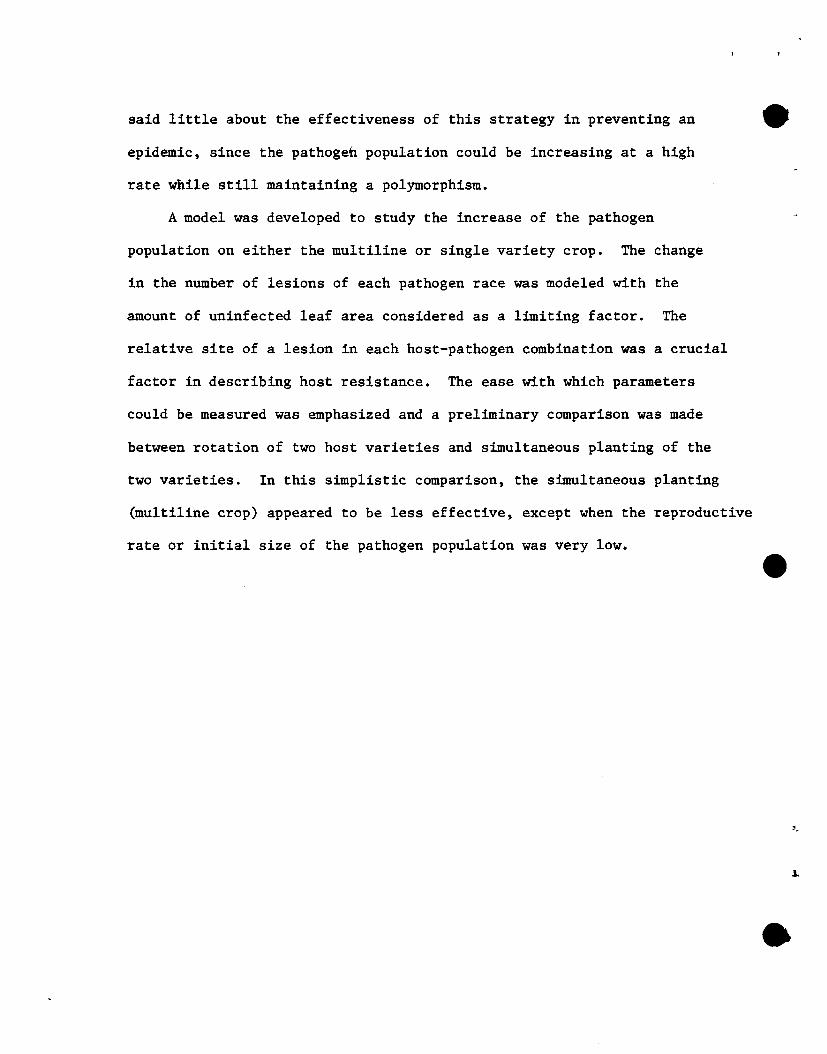
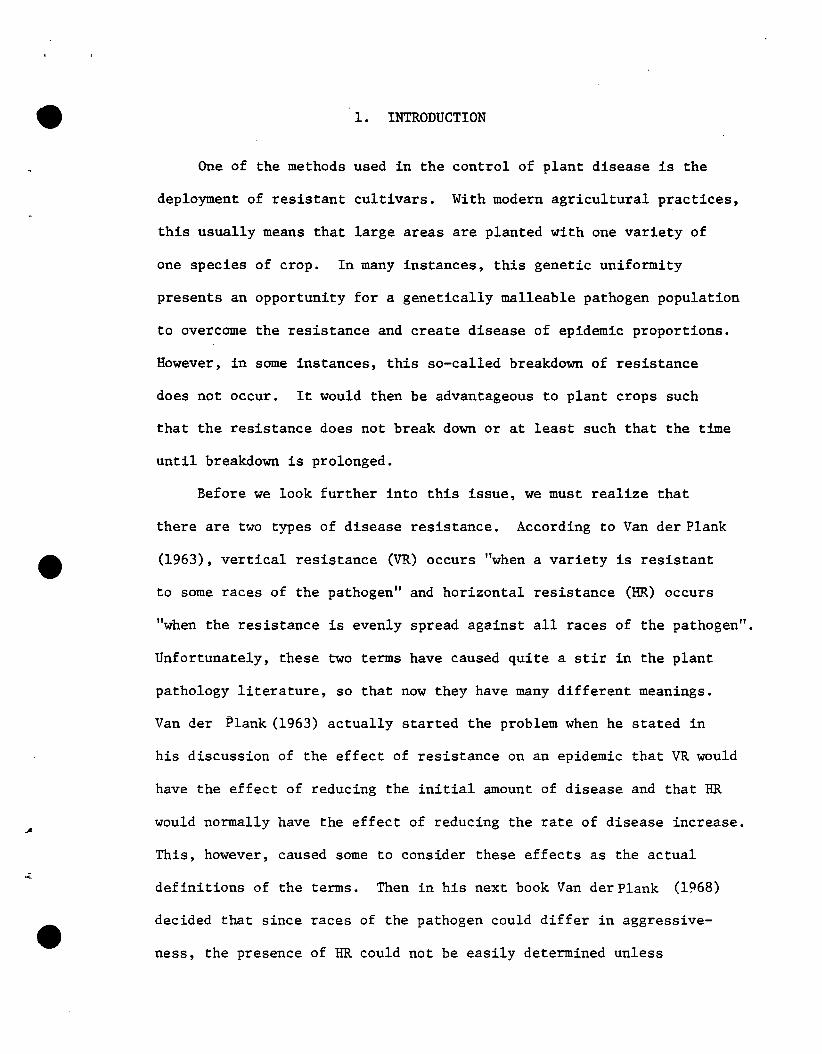
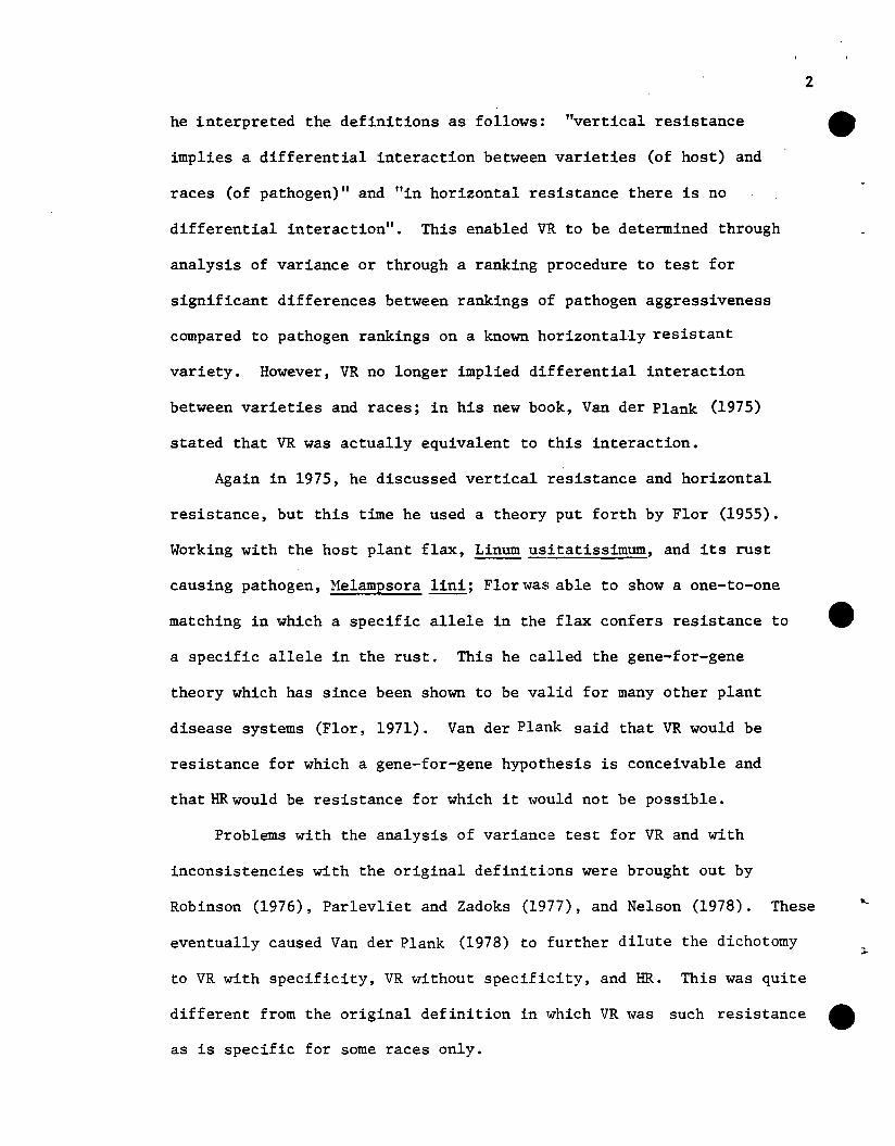
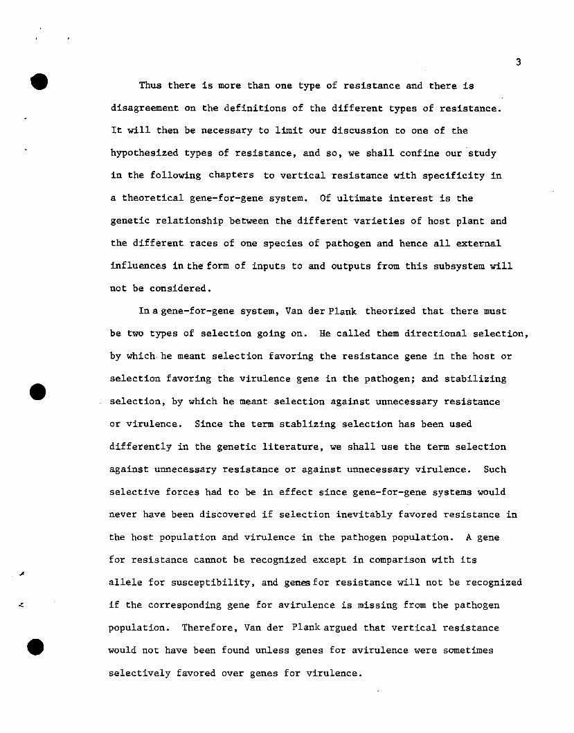
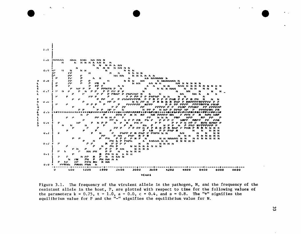
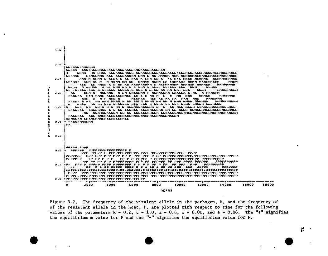
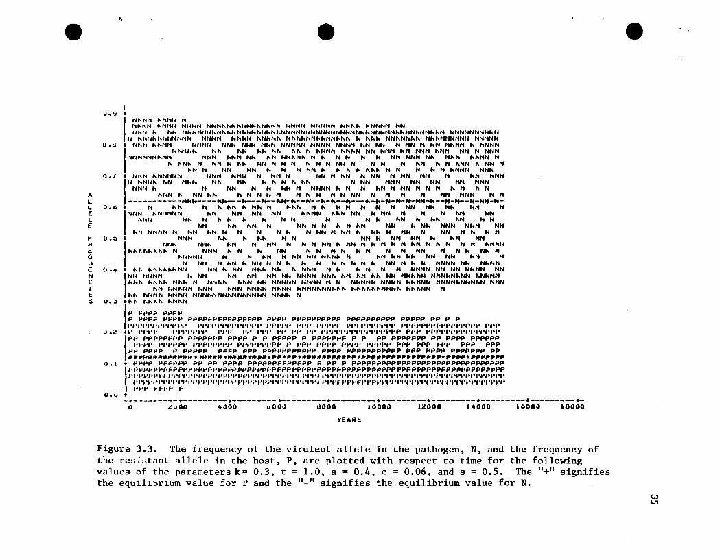
us first to resort to numerical studies. The following set of figures

(Figure 1 through Figure 3) graphically represent the results of a number

of those computer simulations of the system (3.5) for various parametric

values. Notice that for most of these simulations there is a marked ~

spiralling in toward the equilibrium point with increasing time. Hence,

it appears that, for at least some region of the parameter space, the

internal singular point is stable or at least there exists some stable

limit cycle about that point.

In any event, it does appear that the forces of selection against

unnecessary resistance in the host are enough to account for the observed

polymorphic populations of hosts and pathogen; if not at a stable

equilibrium point, then at least in some stable cycle.

The above analysis would have been enough to show the explanatory

power of Van der Plank's concept, but Fleming (1980) published a model

which he claimed to be a continuous analog to Leonard's discrete model.

e " e e

N/Ii

NNN NN

N

tI

p

NIII N

N NN N

N

'" NNN NN N NN N N

N '" N NN N ... N ... N

N /ioN NNNNNN NN N N NN N NNNNNNN N

N N NN "N N N HN N N N N NP N N 1\ N N N NNN N N N N N N N N NPPNPN P N N N N N NNN N N N N N NPP .... PP N N NN N N

P P pNNP P PNPFNP N N N NI\ NN iii NP P P PP P P PNPNP N N N N N

I' P PN"'PPPPP" P P R P P P PNR P P P R PN N N NPP I' N N PP N P R R R R PNP P NRPPPPNPPPPP P P

P PPPPPPP "PPp P P PP pPflP PPPP,...P,. PRNPp P PP PP PPPPP P P PNNp pPNRp PP PPPPPP

N

PHPP

PP

PP

P ppN

/10

N

Pppp

p

pp

p p P

"p

N N

NNN "'N NNN N N 1\ "'N

N NN

pppp

P

NP PP N

P

N

P

p

p

NNNN

NPPppPI-'ppPI'PI'

P

fl

p

N

I•IrNM~

...I~ .,i ~." NI .,., ..

P I' P P NP P N N PP P N NP P PPNP NP P PPNNPMN PM.~~~~~;~~ •••••••••M~•••+++_ t•••••+.+••+•••••" +.I N P P PPN P H N RP NR PPPPP AN P PPN P R NPN NRP

I' .. PI' N N N P P PP III N III PRP NPP "P PP PP PP III N P P P" Ph PI' P P P NHPP AftPP PP PPR

• P liP P N P P N P PI PN P .. P P P P N PP P RPN NPRP P, N N N P P N FN P N P P N P PNP NPPPPPPP P

P P P flP P P P PP N P P .. N P R AhP P PNR P R R N N N NF P P P P 1\" P P PNP R N N N N N

• F P N P PNPP P H PNP P PNPN N N HN N N N N

I PP P NN PNP R P R N N N N N N N N Np P P PN P P P P N P N N N NNNNN N N N N N N N N N

P N PN /Ii P PNP,.. '" "'N"h'" N N N N N N N• P PP" PPPP N N NNNN

)

I' P N PNP NNhN/liNNNP N P P P P P NN N N N N

I' h "NN PN P P N N N N N• P N PN N N 1\ N N

I ~ F N PP .. P N N /liN NN ~ PN P PN NN N '"

P "'P PP PPN ..N N NN• PPHNN PHNN PNN N-t-------.-------t-------t-------t-------t-------t-------t-------t-------t-------t-------t---o oou 1200 1800 ~.oo ~ooo J60G 4200 4UOG 5400 6000 6600

1 .1

1 .0

O.~

II. u.uLLEL 0.1to

I'I~ U.oLauf: u.:>'"(.

1f: U."S

U.J

o •• L

0.1

u.u

~e"Hi

Figure 3.1. The frequency of the virulent allele in the pathogen, N, and the frequency of theresistant allele in the host, P, are plotted with respect to time for the following values ofthe parameters k = 0.75, t = 1.0, a = 0.0, c = 0.4, and s = 0.8. The "+" signifies theequilibrium value for P and the "_" signifies the equilibrium value for N.

ww

0.'01

O.U

0.1

ALL U.oELt:

t= 0.5kEauI: 0.'0NCIES O• .J

0.,

0.1

0.0

I

ItIhN"NNNM,NN"NN

N/'IoNNN "NN"NNNNNNN~""NhNNN"'NNN"NN"NNNN"NNNNN

N UNNN NN NNNN "'IIiN",..NNNNNN N""t4NNN"NN,,"""""N"""NNN"NNh"NNNNNNN"NNN"'NNNNNNNNNNN N"NNNNNN """ "hNNhNNNN tlNtI N NN NNNNN NNN NNNNNNNNNNNNNNNhNNN"NNNNN

t NlliN N NNNN N ""N" N "" N"N " ""'N NN" "" ""''' NNNN NNNNNN NNNNNNNNNNN

lNM'NN" NNN NN N N NNNN NN NN NNNNN NNNN hN "NNNhNN NNNN N"N"NNNNN NNNN""" "... NNNN " N NN "N ""IIiN"IIiNNN N N"NNNNNNN NNNNNN NNNNNN NNNNNNNN

NNNN N NUIINN N N" NNN NN N " NNN N IIi"'N" "h"""''' "NN NNN "NNN"1Ii"'--"''''''''''-''H''-H-H-h'''''h-hHN'''H-h-NNh-N-H-NN-NN-NN-NH--NNh---NNHH-----HNNNHHNNN

t ... h NNN N NNNNNN N NN HNhNNhN N NHN"'''NN''' N"'N"NN ... N'" iii "hNN"N

IN/\N..."h NI\N NNNN """N"NNNNNN "N " N NN N N '" NN NNN NNNNN NNNNNNNNNN N N N NNN N N"NN"N N"N "" "... "... ... ...N NNN "'NNN"NN

....... hN" iii N.... HN "'NN NNNN N NN I'oNNN NNNN NN NN N NNN NNNN NNNNNN I'oNNN"NNNNNN N"'NN NN NN N"" N""'NN"'" N/\N ""'N N NN"'''' "'" N"'''' NNNN NNNNN NNNNNNN

tN NN/\ NN NN N N N NN N NNNNNN"''''NNHN N N "N N"N N"NN "NNN"NNN"NNN"NNNN

IN/\"'N""" "N"'NNNNN" N NN ""'NN"N """''''N''N'''''N NN NN NNNN NNNNNNNNNNNNNNNNNNNNNNN NNNNNNIIi"NNN NN NN "NNh"NNN"NN ~""'''''NNNNNNNNNNNNNNNNNNN''NNN''NNNNN

N.... hN"'........ "NN NNNN""""'I\NNNI\NNNNNNNNNNN"NNNNNNNNNNNNNNNNhN NN"NNNNNNN""I\NI\"NN~~iN:NNNNNNNN'"

t

) "'1'1'1"1" pl''''Pt IiPPPPF PPPPPPPPPPPPPPPPP PI PPP PPPPP P PPPPPPPPPPPPPPPPPPPPPPPPPPPPPPPPPP PPPP

IPPPI'/'PP PPP ppp PPP PPP PI' P PPP PPP P PP PPPPPPPPPPPPPPPPPPPPPPPPPPPPPPPPPppppppp fp PI' I' I' I' PI' P P PPPPP P PPPPPPPPPPPPPPPPPPPP pppppppppp

1'1'1' PP PI' P P PPPPpPPPJ> PPP PP PPPP"P PI' FPP PPPP PpPP..P PPPPPPPPPPtI'l-' "PP I' PPPPP PPPP PPPPPPPP F P P P PI" I' PI' PP PPP PPP PPPPPPPPP

(

PI' PP P I' PP PPPPP PPPP P P P PP I' PI' PP PPP PPP PPPPP PPPPPPP~~~~~~~~~t~•••~w•••w••• t •• t.W••WWt.t•••• tW.t•• t •• t •••• t ••••ptt••••••••••••••

PfOpP pppppppppppppppppppppppppppppppPPPPPFPPPPPPFPPPPPPPPPPPPPPPPPPPPPPPPPI>PPPPFPPPpPppppppppppppppppppppppppppppppppppppppppppppppppppppppppppppppppp

tPPPPPPPPPPPPPPPPPPPPPPPPPPPPPPFPI'Pp-t---------t---------.---------t---------t---------t---------t---------.---------.---------t-

o ~OOO 4000 t.000 11000 10000 12000 a4000 16000 18000

YCARS

Figure 3.2. The frequency of the virulent allele in the pathogen, N, and the frequency ofof the resistant allele in the host, P, are plotted with respect to time for the followingvalues of the parameters k = 0.2, t = 1.0, a = 0.6, c = 0.01, and s = 0.08. The "+" signifiesthe equilibrium m value for P and the "_" signifies the equilibrium value for N.

eI'

e ew.J:-

e

o.~

o.u

0."

ALL 0.6ELE

t' 0.::>..£Q

uE 0.4NC1f:::i o.~

0.;:'

0.1

O.U

t,

e

I•

INtoNN hNNU NNNNN NNNN NNNN NNN"toN .... NNN"NN"'.... NNNN N....N.... '" N"'''.... "N"'NN NNNtoN" M~ NhNNtll~"N"""'N"'NN.... NNN"NNNNNNNNNNNNNNNNNNNNNNNNNNN"NNN"N NNNNNNNNNN

N "NNN"hNNNNN NNNN N",NN "NNN" N"''''''NN''''''''N'''''' " "",,,, NN"N"''''" NN"NNNNNN NNNNN• NhN NNNN NNNN NNN NNN NNN NNNNN NNNN NNNN NN "'N N NN N NN N........N .... "'NNN

,N"NNN N" hN ",,, .... ,, "" N "NN'" hN"N NN NNN NN NNN NNN NN N NNN

NNNNNNNNN NNN toNN NN NN NN"N.... N N N N N N N.... NNN NN NNN N",NN N.... "N.... N NN N "" NN N N N N N N NN N N N N "N '" N NNN " NN N

NN N NN NN N N N "N N """ """ N" N N N NNNN NNN• N"N NNNNNN NNN NNN N NN N NN N toN N NN N NN NN N NN NNN

IN "'Nr~ .... "N NNN N", N" '" iii N to ",N N NN NNN NN NN NN NNNNNN N N ....N N N NN N NNNN" N N NN N NN N N N N N '" N

"hN" "'.... NN h N N N.... .... N N N N NN N N N N NN NNN N N-----------NHN----Hh---H_--H_-~N-~--H_-N-~--H_--~-N-H_H_H_NH-N--N-N--N-NH-H-

• .... N", N" "" .... Nh.... N"" N N .... N N N N NN NN NN NN N

,NNN NNlmNN NN NN NN NN NNNN ""N NN N NN N N N",N NN

",NN NN N "''' '" N N N N N N hN h N" "N N N....N "N ....N N ........ N N "N "N NN N NN NNN NNN NN

NN NNhN N NN NN N N N N N N NN N NN" NN N NN N NN N N N N.. NNN",,,,, "N N N NN N NN NN N NN NN

J

NNN NNN NN N NN N N N NN N NN N N N N N NN N .... N N /It ....NNNN"'''hN'''''' N NNN" N '" NN N N N N N N N N NN N N N NN N

"NNNN N N NN N "'N ....N N" .... " .... "N NN NN NN NN NN NN NN N NN N NN N N N N N N N N N '" NN N N N NNNN NN NN"'N

t 1'4" """"NN~~ NN "NN N" .... N" " ...."'N N", .... N N N NNNN NN NN NNNN NN

iNN Nlm.... N ....N ".... NN NN NN NN N N"''' "'N "N N.... NN NN"NN NNNNN"....N "N....NNNN" N""" N"N N NN"" ,.,"N ....N N....NNN N NN N N NNNNN NNNN NNNNN NNNN"NNN"'N .... NN

"N NN"NN "NN ",NN NN"N N",NN "'NNN"NN""'" """'''''''NNN'' N"''''NN NNN NN .... '" NN ....N NNNNNNNNNNNNNNN N"'NN N

.",N "",," NN"N

JP ".IPP PPP PP P.,PF PPPP pPppFPFPppPpppp PPPP PPPPPPPPPP pppppppppp PPPPP PI" I" I"pppppppppppp PPPPPPPPPPPPP PPP~P PPP PPPPP PpFpPPpPpp ppppppPFpPpppPPP 1"1"1"t" P..pfi ppPpf>PP 1"1"1" PI" PPP PI" PI" PI" PPPPPPPPPPPPPPPP 1"1"1" PPPPPPPPPPPPPPP

IPP PPPPPPPP pppppr'p PPPP I" P pFppp I" pPpPppF P I" PP ppppppp PI" 1"1"1"1" 1"1"1"1"1"1"

PFpP PPPPPP pppppppp PPPPPPPPP P ppp PPPP PPPP PPPPP PPP PPP Fpp ppp pppPP PP~P I" PPPPP PFFp 1"1"1" pPpFPpppPPP PPPP PPPPPPPPPPP 1"1"1" 1"1"1"1' PPPPPPP PI"~~_~__M~~~~~~ ••~~WW.H•••••_W.ww••• +w.ww••••••• ,w•••••, ••••••~•• t ••••+•••••••

• PPPP PPPPPP PI" PI' PPPP ppppppFppPPPP P PI" P PPPPPPPPPPPPPPPPPPPPPPPPPPPPPPP

)/'l'fiPPpPPPPPPPPPPPPPPPPPPPPPPPPPPPPPPPPPPPPPPPPPPPPPPppppppppppPpppFPPPPPPPPPI'PPPPPfpPPPppppppppppppppppppppppppppppppppppppppppppppppppppppppppppppppppp

P/'/,f'PPPPPPPPPPPPPPPPPPPPPPPPPPPPPPPppPPPFFPPFFpppPPPpppppppppppppppppppppppI ppp fi .. .,p F

•-+---------.---------t---------.---------+---------+---------+---------.---------.---------+_o .lOOU 4000 oOl)lJ tlOOO 10000 12000 14000 16000 18000

YEAR:.

e

Figure 3.3. The frequency of the virulent allele in the pathogen, N, and the frequency ofthe resistant allele in the host, P, are plotted with respect to time for the followingvalues of the parameters k= 0.3, t = 1.0, a = 0.4, c = 0.06, and s = 0.5. The "+" signifiesthe equilibrium value for P and the "_" signifies the equilibrium value for N.

W\Jl

36

Fleming was able to construct a Lyapunov function for his continuous ~

model and to show that the internal singular point for his-model was

globally a center. It is not necessarily true that the solution of a­

differential equation, developed in the same manner as a difference

equation, will be qualitatively the same as the solution of that

difference equation (see van der Vaart, 1973). In the case of

Fleming's model versus Leonard's model, this is obvious from the computer

simulation of Leonard's model that demonstrates a-spiralling in effect.

However, it is more compelling and mathematically more attractive

to obtain an analytical proof of this fact and that will be attempted

in the next chapter. We would like to show that our internal singular

point for system (3.5) is not a center, but a focus. Although there

are many techniques for doing this in differential equations, the only

method that appears to be applicable to difference equations as well, is

that developed by Poincare (1885). All the others appeal to the fact ~

that trajectories in continuous-time cannot cross and thereby appeal to

the Poincare-Bendixson Theorem in some form.

In the next chapter, we shall describe Poincare's method, adjust

it for difference equations, and apply it to determine whether the

internal singular point in Leonard's model is a center or a focus.

37

4. THE CENTER-FOCUS PROBLm1

It is well known that for a system of two nonlinear differential

equations, if a singular point is a center for the linearized system,

then it is a center or a focus for the original system (Coddington and

Levinson, 1955, p. 382). A method for discerning a focus from a center

by using higher order terms of the Taylor series expansion for the

nonlinear equations was described by Poincare (1885). The analog of this

method for a system of two nonlinear difference equations will be dis-

cussed here. Although the methods are analogous, some difficulties will

arise in difference equations that do not arise in continuous systems.

Suppose, ir the first place, that. the system of two nonlinear dif-

ference equations has been transformed so that the singular point is at

the origin (0,0). Then the system (S) can be written as the following:

ex' = x(t+l) = g (x(t) ,y(t» = g(x,y) = gl (x,y) + g2(x,y) +

y' = y(t+l) = h(x(t) ,y(t» = h(x,y) = hI (x,y) + h2 (x,y) +(8)

where g. and h. are homogeneous polynomials of degree i in x and y. If~ ~

the singular pednt in the linearized system is a center (1. e., the

eigenvalues of the Jacobian matrix of g and h, and in fact, of gl and hI'

evaluated at the singular point have modulus equal to one), then the

singular point of the nonlinear system (8) is either a center of a

focus. To discover whether the singular point is a center or a focus,

we will try to construct a continuous function

38

whose contour lines, f(x,y) = C, constitute a family of closed curves

such that either

(1) f(x,y) is constant along the solution curves of (8)

or

(2) f(x,y) changes monotonically along the solution curves of (S).

Actually, f(x,y) is just a Lyapunov function where the f. are homogeneous1

polynomials in x and y of degree i.

In order to judge whether the system is a .center or a focus, we

must investigate the function, f' , which is defined as follows:

f' (x,y) = f(x',y') - f(x,y).

As in Lyapunov's direct method, if f' = 0 for all values of x and y, then

f is constant along the solution curves of (S),and we have a center

since f has been constructed to constitute a family of closed curves.

On the other hand, if f' > 0 «0) for all values of x and y except the

singular points, then f is monotone increasing (decreasing) along the

solution curves of (8), and we have an unstable (stable) focus. The big

difficulty in using Lyapunov's direct method lies in finding a suitable

function f; however, in the following method for the center-focus problem,

an algorithm for a stepwise construction of ,i suitable f is given.

Recall that f' was defined as follows:

f'(x,y) = f[g(x,y), h(x,y)] - f(x,y) =

= {f2[g(x,y), h(x,y)] - f 2 (x,y)}

+ {f3[g(x,y), h(x,y)] - f 3 (x,y)} + ...

39

For notational convenience, we shall make the following definition.

Define fij(x,y) to be the homogeneous polynomial of degree j in x and y

that results from f.[g(x,y), h(x,y)] such that:1.

00

fi[g(x,y), h(x,y)] = !: f ij (x,y) •j=i

Here is where the method for difference equations gets more complex

than in Poincare's differential equations. It becomes an extremely

difficult accounting problem to keep track of the various terms, yet we

are able to solve this problem in the following way:

00 00

f' (x,y) = {[ !: f 2j (x,y)] - f 2 (x,y)} + {[ !: f 3j (x,y)] - f 3 (x,y)}+ •••j=2 j=3

And then we rearrange to obtain:

If we then define f'i as follows:

f'.(x,y)1.

=i

{[!: fa (x,y)] - f i (x,y)}[=2

(4.1)

...we can break f' up into:

f' = f' + f' + f'2 3 4 + ...

where f'. contains all terms of degree i in x and y in f' •1.

40

Thus for a system with a specific g(x,y) and h(x,y) that has a ecenter for its linearized system, we shall try to construct an f such

that f' = 0 for all values of x and y. Note that f' = 0 will not be

true for all values of x and y, unless f'Z = 0 for all values ofx and

y. Otherwise, in a small enough neighborhood of the origin the higher

order terms would not be able to compensate for f'Z not being equal to

zero. First then, to start our construction of f, we must choose f Z

so that f'Z = o. By the same argument as above, once we have f Z ' we

need to choose f 3 so that f' 3 = 0 •. Ir_we can continue to choose f i so that

f'i = 0 ad infinitum, we could construct f so that f' = 0 and thus prove

the existence of a center. This is in general quite impractical and so

the main use of this method is in disproving a center. To this end, we

hope to arrive at a step in which f i cannot be chosen so that f'i = 0

and in this case, we shall choose f i so that f'i is definite for all

values of x and y.

The only other requirement that f must fulfill is that f(x,y) =

fZ(x,y) + f 3 (x,y) + f 4 (x,y) + ... be a continuous function whose contour

lines f(x,y) = C , produce closed curves. Poincare (1885, p. 178) showed

that if fZ(x,y) = kZ ' with kZ a constant, rE~presents a closed curve,

then within a small enough neighborhood of the origin, f(x,y) = k , with

k an appropriate constant is also a closed curve. Since in our case, the

linearized system gives a center, we know that the contour lines, fZ(x,y)

equals k2, are closed curves, therefore, within a small neighborhood of

the origin, f(x,y) = k produces a closed curve.

defHence, we will have constructed a function f*(x,y) = fZ(x,y) +

f 3 (x,y) + ... + fi(x,y) , whose contour line. f(x,y) = k , within a small e

41

neighborhood of the origin, is a closed curve and such that f*' = f'Z +

f'3 + ... + f'i is either negative definite or positive definite.

The terms up to degree i that are involved in the function f' will

be all present in f*(x' ,y') - f*(x,y) . Here x' and y' are expressed by

the following truncated version of (S) which we shall call (S*).

x' = g*(x,y) = gl(x,y) + gZ(x,y) + gj(x,y)

y' = h*(x,y) = hI (x,y) + hZ(x,y) + ... hj(x,y)(8*)

where j < i. In fact, in order to include all possible terms of degree

i that come from f*(x' ,y'), we need j such that j = i-I.

This is so since for fZ(x' ,y') = aZ(x')Z + bZ(x')(y') + cz(y')Z

the terms of degree i that are produced are a Z(Zhl hi_

1) + bZ(h

1g

i_1 +

glhi-l) + cZ*Zglgi_1)' Thus if we work with a truncated version of (S),

it must be (8*).

Now that we've constructed f* so that it represents a closed curve

and so that f*' is definite, the questions that remain are how does

f*(x,y) behave along the solution curves of (S*) and is it comparable

to the behavior of f along the solution curves of (S)? These questions

can be answered by the following theorem, the proof of which resembles

Theorem 9.14 in laSalle (1978).

Theorem: If f*(x,y) = fZ(x,y) + f 3(x,y) + ... + fi(x,y) = k is a closed

curve and if f*' = f'Z + f'3 + ... + f'i < 0 , then f(x,y) = fZ(x,y) +

f 3 (x,y) + ... is a Lyapunov function for (S) and the origin is an

asymptotically stable point of (S).

Proof: For (S*), we have the following:

42

f'S*(x,y) d~f f*[g*(x,y), h*(x,y)] - f*(x,y) = {f2[g*(x,y), eh*(x,y)]- f 2(x,y)} + {f3[g*(x,y), h*(x,y)]- f'3(x,y)} + ••• + {fi[g*(x,y),

h*(x,y)]- fi(x,y)} = f'2 + f'3 + ••• + f'i + terms of degree larger than

i up to terms of degree ij = f*' + (higher-order terms).

Since the coefficients of these terms of degree larger than i are

all finite, we can choose a small neighborhood of the origin such than

for (x,y)in that neighborhood, f'S*(x,y) < 0 when f*' < O. Thus f*(x,y)

is a Lyapunov function of "(S*) in this region of the origin and hence

the origin is an asymptotically stable point of (S*). Now, write (S) as

fo11Clws:(

x' = g(x,y) = g*(x,y) + gj+

y' = h(x,y) = h*(x,y) + hj +

where hj + and gj+ are polynomials in x and y of degree higher than j.

Then:

f'S(x,y) = {f[g(x,y), h(x,y)] - f(x,y)} = {f2[g(x,y), h(x,y)] ­

f 2(x,y)} + {f3[g(x,y), h(x,y)] - f 3(x,y)} + ••. + {fie g(x,y), h(x,y)] ­

fi(x,y)} + {fi+l [g(x,y), h(x,y)] - f i +1 (x,y)}+ •••

And so, f'S(x,y) = f'S*(x,y) + terms in x and y of degree higher than i.

This is so since the addition of gj+ and hj + to g*(x,y) and h*(x,y) in

(S*) adds on a polynomial with lowest degree terms as follows:

a2[2g1 (x,y)gj+1 (x,y)] + b2[gl(x,y)hj +1 (x,y) + gl (x,y)hj +1 (x,y)] +

c2[2h1 (x,y)hj +1 (x,y)].

The above polynomial of degree i+1 is arrived at in the following manner:

f 2[g(x,y), h(x,y)] = a2 (g* + gj+)2 + b2(g* + gj+) (h* + hj +)

43

+ b2[(g*h*) + (g*hj +) + (h*gj+)

+ (gj+hj +)] + C2[(h*)2 + 2(h*hj +) +(hj~)2]

+ terms of degree j + 2 and higher. Here

j+ 2 = i + 1 •

Once again, we can choose a neighborhood of the origin such that

for x and y in the neighborhood, if f'S*(x,y) < 0 , then f'S(x,y) < 0 •

And since we've shown that in a small enough neighborhood of the origin

f'8*(x,y) < 0 if f*' < O,weneed only choose the smaller neighborhood

to get f'S(x,y) < 0 and hence the origin is asymptotically stable for

(8) •

An analogous proof can be used to shown that the origin is an

unstable point of (8) if f*' > 0 •

80 if we construct f*(x,y) = f 2(x,y) + f 3 (x,y) + ••• + fi(x,y)

such that f*' = f'2 + f'3 + f'4 + ••• + f'i is either positive or

negative definite, we can sho~~ that the origin is either an unstable

or asymptotically stable singular point for the system (8). And the

region of attraction will at least be the smallest neighborhood of the

origin which satisifes the-following: (1) f*-(x,y) = k is a closed

curve, given that f 2 (x,y) = k2 is a closed curve, (2) f's*(x,y) has the

same sign as f*' for values of x and y in that neighborhood, and (3)

f'S(x,y) has the same sign as f's*(x,y) in that neighborhood. Notice

also that this neighborhood will be larger than that used in the linear

analysis, since the neighborhood in the linear analysis is small enough

to disregard the higher order terms and here, we are considering a

neighborhood in which these higher order terms have an effect.

44

One problem that arises in the difference equation case, does not ~

arise in Poincare's study of differential equations. That is, in

calculating f'. for the difference equations, we automatically generate­~

higher· order terms, whereas for differential equations in which we have:

f' =i

i-2l:

j=O{Cd fi...j(x,y)/d xJ8j +1 (x,y) +

+

the higher order terms are not generated. This makes the study of

differenceequatj.6nsvery cumbersome and, as has been seen, it complicates

the notation. It also requires an additional neighborhood argument

(i.e., see point (2) in the preceding paragraph).

Because of the trouble with keeping track of the higher order terms,

it is instructive to see the application of this method in all its

detail; however, inthe interest of readability, most of this detail

shall be relegated to Appendix 8.6. The method will be applied to

Leonard's model to determine if its internal equilibrium point is a center

or a focus. Recall that Fleming (1980) developed a so-called continuous

analog to Leonard's model, showing the singular point to be a center, and

computer simulation of the alternate steps version of Leonard's model that

was presented in the previous chapter, appeared to show a stable focus or

at least a stable limit cycle. Thus we would hope to prove by this method

that the internal singular point of the alternate steps version of Leonard's •

model is not a center, unlike that of Fleming's model.

45

First, we shall write the equations of the alternate steps model

in the following expanded form via a Taylor series expansion where x arid

yare deviations from the singular point at the origin. Using x' =

x(t+l), y' + y(t+l), x = x(t), and y = y(t); we have the following system

(5) :

y' = h(x,y) • Llx + (1 + LlKI)y + (LlKZ + LZ)XY +

Z Z+ (LlIS + LzKI) y + (L3~ + Ll K5 + L4 + LZKZ)XY

where the Ki and Li as' well as Cl are all functions of the original

parameters. The actual expressions are given in Appendix 8.7.

ZTo implement the method,we must first find fZ(x,y) = aZx +

ZbZXY + czy such that equation (4.1) with i = Z yields:

It is seen in Appendix 8.6 that this will be zero for all values of

x and y if we choose aZ = Ll , bZ = LlKI, and Cz = -~. Thus fZ(x,y)

equals LlXz + LlKlxy - KIyz. This will be a closed curve if its

discriminant, ~l~r+ 4Ll KI < o. This is true since for biologically

realistic parameter values as suggested by Leonard Ll < 0 and KI > 0

46

So we have found fZ(x,y) such that f'Z = 0 for all values of x

and y and fZ(x,y) = "constant" is a closed curve. Now we can evaluate

fZ(x' ,y') to get our terms of higher order (i.e., f Z3 (x,y), f Z4 (x,y),

... ) .Next we must find f 3(x,y) = a3x3 + b

3X

Zy + c3xyz + d3y3 such that

equation (4.1) with i = 3 yields:

Appendix 8.6 shows that this will be true if we choose the

following:

Za3 = (1/3Ki){-ZLl C3 - 3Ll d3 - Gl }

Zb3 a -{Ll C3

+ Ll d3}

c3 = -{1/[(1/3)Ll KiZ + K~J} {(ZI3)KiZGl - KiGz + G3}

2d3 = -{l/[Ll Kl + 3Ll J} {GZ - KiGl }

where

G =1

Since IKlLl ! < 3 as seen in the previous chapter, we do not have to worry

about zero in the denominator, and so we can choose a3 , b3, c3 ' and d3

that satisfy f' = 0 •3

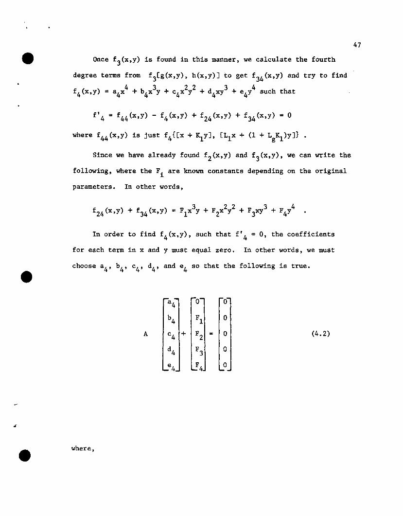
Once f 3{x,y) is found in this manner, we calculate the fourth

degree terms from f 3[g{x,y), h{x,y)] to get f 34 {x,y) and try to find

4 3 2 2 3 4f 4{x,y) = a4x + b4x y + c4x Y + d4xy + e4y such that

Since we have already found f 2{x,y) and f 3{x,y), we can write the

following, where the Fi are known constants depending on the original

parameters. In other words,

In order to find f 4{x,y), such that f'4 = 0, the coefficients

for each term in x and y must equal zero. In other words, we must

choose a4 , b4 , c4 , d4 , and e4

so that the following is true.

a4 0 0

b4 Fl 0

A c4 + F2 = 0 (4.2)

d4 F3 0

e4 F4 0

where,

47

48

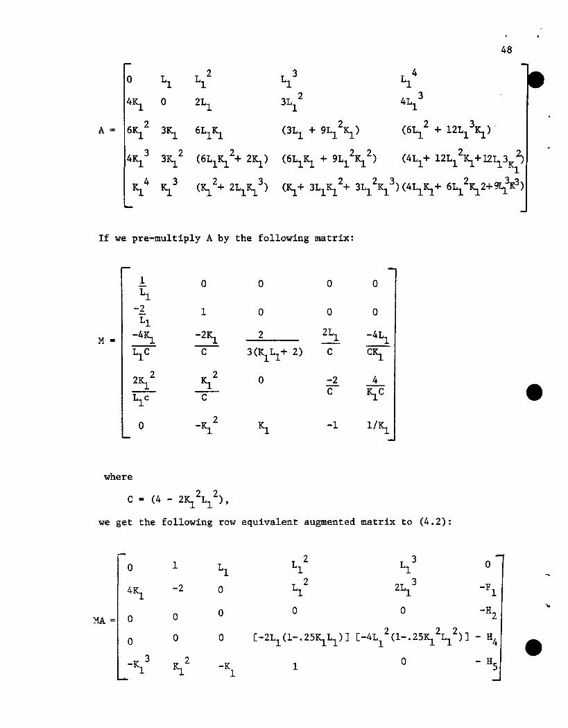
0 LlL 2 L 3 L 41 1 1

4IS. 0 2Ll3L 2 4L 3

1 1

A = 6IS.2

3IS. 6Ll IS. (3Ll + 9L12IS.) (6L1

2 + l2L13IS.)

4IS.3

3IS.2

(6Ll IS.2+ 2IS.) (6Ll IS. + 9L12~2) (4Ll + l2L1

2IS.+ 12S.3 ~Kl

~4 IS.3 (IS.2+ 2Ll IS.3) (IS.+ 3Ll IS.2+ 3L1

2K1

3) (4Ll IS.+ 6L12IS.2+~~3)

If we pre-multiply A by the following matrix:

1 0 0 0 0Ll

-2 1 0 0 0Ll

M= -4IS. -2IS. 2 2Ll -4L1LIC C 3(l<lL1+2) C CIS.

2IS.2

IS.2 0 -2 4

LIe C C IS.C

0 _~2 Kl -1 1lIS.

where

we get the following row equivalent augmented matrix to (4.2):

0 1 LlL 2 L 3 01 1

4IS. -2 0 L 2 2L 3 -F1 1 1

0 0 0 0 -HMA= 0 2

0 0 0 C-2Ll (1-.2SIS.Ll )] C-4L12(1-.2SIS.2L12)] - H4

-K 3 ~2 -K 1 0 - H1 1

5

49

Here H2 = (~Ll- 2)(F2/3) + RiFl - L1F3 + [2Ll/~]F4 and H4 and

H5

are comparable functions of Fl , F2 , F3 , and F4 •

All row operations are legitimate since neither Ll nor K1 is

zero and IL1~1 < 2. Thus A is singular and (4.2) cannot be satisfied;

so we must attempt to make f'4 definite. To do this, we first rearrange

A so that row 3 is now row 5 and the other rows remain in order. Hence,

we have the block matrix A* with A1245 consisting of rows 1, 2, 4, and

5 of matrix A, on top and A3

, or row 3, on the bottom, and we have

Since A is singular, A* is singular, and we cannot satisfy A*a - f = O.

We can see that A1245 is a 5x4 matrix of rank 4 by performing

elementary row operations as indicated in Appendix 8.8. With A1245 of

rank 4, we can choose a such that (A*a)i- f i = 0 for i = 1, 2, 3, 4 or,

in other words, such that

5or aijaj = f i for i = 1, 2, 3, 4 •J=l

(4.1)

(4.4)=

4 3 3 4Thus we can choose a such that the coefficients of y , y x, x y, and x

are all zero. The value of the coefficient of x2y2 is:

51: aSJoaJo-fS

j=l

We have from MA that the following is true with gl = m3l ,

g2 = m32 , g3 = m34 , and g4 = m35 , where the m3j for j = 1,2,4,5 are from

matrix M.

o =

so

which implies that

=

Thus, we can calculuate (4.4) as follows:

which from equation(4.3) is equal to the following:

= [-3(RILI + 2)/2J

= 3- - (K-L + 2)(-H )2 -1. 1 2

Since -2 < KILl <,0 for most parameter values that we would expect

to produce a stable equilibrium point (see Chapter 3), we can see that

the coefficient of x2y2 has the same sign as H2 • Thus, we have chosen f 4

such that f'4 is definite with the sign of HZ' The system's singular

point will be a locally stable focus if HZ < 0 , and a locally unstable

focus if HZ > O. If HZ = 0, then, we must go on finding fi(x,y) such

that f'i = 0 until we can disprove our center. Unfortunately, the general

expression for HZ in terms of the parameters requires an intractable

number of terms and is therefore impossible to investigate by analytical

means. Hence, it needs to be numerically calculated for various values

of the parameters in order to get an idea ofits sign. The values for

differential parametric values are given in Table 4.1.

...

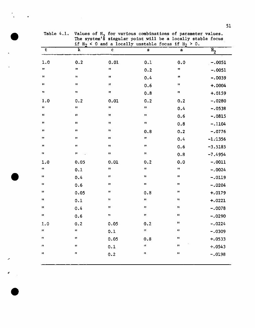
51

Table 4.1. Values of H2 for various combinations of parameter values.The system's singular point will be a locally stable focusif H2 <: 0 and a locally unstable focus if H2 > O.

t k c s a H2

1.0 0.2 0.01 0.1 0.0 -.0051

" " " 0.2 " -.0051

" " " 0.4 " -.0039

" " " 0.6 " +.0004

" " " 0.8 " +.0159

1.0 0.2 0.01 0.2 0.2 -.0280

" " " " 0.4 -.0538

" " " " 0.6 -.0815

" " " " 0.8 -.1104

" " " 0.8 0.2 -.0776

" " " " 0.4 -1 ..1356

" " " " 0.6 -3.5185

" " " " 0.8 -7.4954

1.0 0.05 0.01 0.2 0.0 -.0011

" 0.1 " " " -.0024

" 0.4 " " " -.0119

" 0.6 " " " -.0204

" 0.05 " 0.8 " +.0179

" 0.1 " " " +.0221

" 0.4 " " " -.0078

" 0.6 " " " -.0290

1.0 0.2 0.05 0.2 " -.0224

" " 0.1 " " -.0309

" " 0.05 0.8 " +.0533

" " 0.1 " " +.0543

" " 0.2 " " -.0198

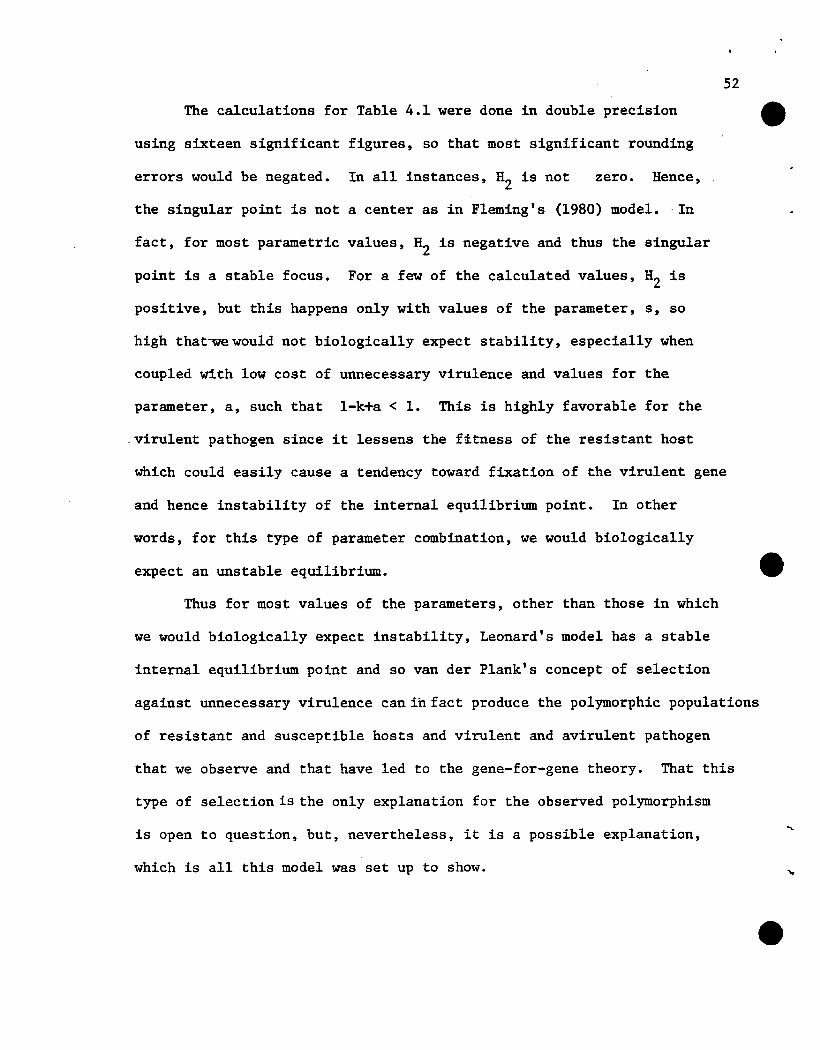
5Z

The calculations for Table 4.1 were done in double precision

using sixteen significant figures, so that most significant rounding

errors would be negated. In all instances, HZ is not zero. Hence,

the singular point is not a center as in Fleming's (1980) model. ·In

fact, for most parametric values, HZ is negative and thus the singular

point is a stable focus. For a few of the calculated values, HZ is

positive, but this happens only with values of the parameter, s, so

high that-we would not biologically expect stability, especially when

coupled with low cost of unnecessary virulence and values for the

parameter, a, such that l-k+a < 1. This is highly favorable for the

.virulent pathogen since it lessens the fitness of the resistant host

which could easily cause a tendency toward fixation of the virulent gene

and hence instability of the internal equilibrium point. In other

words, for this type of parameter combination, we would biologically

expect an unstable equilibrium.

Thus for most values of the parameters, other than those in which

we would biologically expect instability, Leonard's model has a stable

internal equilibrium point and so van der Plank's concept of selection

against unnecessary virulence canihfact produce the polymorphic populations

of resistant and susceptible hosts and virulent and avirulent pathogen

that we observe and that have led to the gene-for-gene theory. That this

type of selection is the only explanation for the observed polymorphism

is open to question, but, nevertheless, it is a possible explanation,

which is all this model was set up to show.

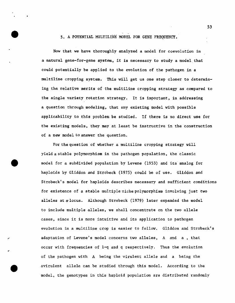
53

5. A POTENTIAL MULTILiNE MODEL. FOR GENE FREQUENCY.·

Now that we have thoroughly analyzed a model for coevolution in

a natural gene-for-gene system, it is necessary to study a model. that

could potentially be applied to the evolution of the pathogen in a

multiline cropping system. This will get us one step closer to determin­

ing the relative merits of the multiline cropping strategy as compared to

the single variety rotation strategy. It is important, in addressing

a question through modeling, that any existing model with possible

applicability to this problem be studied. If there is no direct use for

the existing models, they may at least be instructive in the construction

of a new model to answer the question.

For the question of whether a multiline cropping strategy will

yield a stable polymorphism in the pathogen population, the classic

model for a subdivided population by Levene (1953) and its analog for

haploids by Gliddon and Strobeck (1975) could be of use. Gliddon and

Strobeck's model for haploids describes necessary and sufficient conditions

for existence of a stable multiple niche polymorphism involving just two

alleles at a-locus. Although Strobeck (1979) later expanded the model

to include multiple alleles, we shall concentrate on the two allele

cases, since it is more intuitive and its application to pathogen

evolution in a multiline crop is easier to follow. Gliddon and Strobeck's

adaptation of Levene's model concerns two alleles, A and a, that

occur with frequencies of l-q and q respectively. Thus the evolution

of the pathogen with A being the virulent allele and a being the

avirulent allele can be studied through this model. According to the

model, the genotypes in this haploid population are distributed randomly

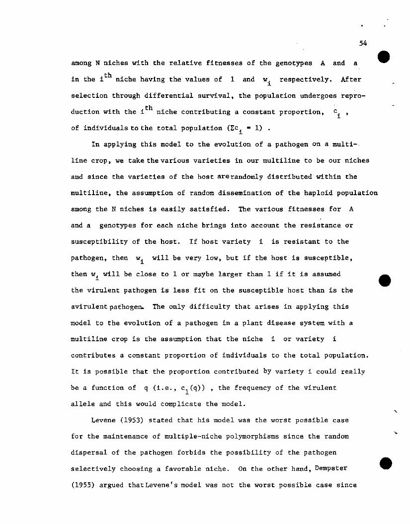
ci '

54

among N niches with the relative fitnesses of the genotypes A and a

thin the i niche having the values of land w. respectively. After~

selection through differential survival, the population undergoes repro­

duction with the i th niche contributing a constant proportion,

of individuals to the total population (1:c i = 1) •

In applying this model to the evolution of a pathogen on a multi-

line crop, we take the various varieties in our multiline to be our niches

and since the varieties of the host are randomly distributed within the

multiline, the assumption of random dissemination of the haploid population

among the N niches is easily satisfied. The various fitnesses for A

and a genotypes for each niche brings into account the resistance or

susceptibility of the host. If host variety i is resistant to the

pathogen, then wi will be very low, but if the host is susceptible,

then w. will be close to 1 or maybe larger than 1 if it is assumed~

the virulent pathogen is less fit on the susceptible host than is the

avirulentpa~hogen. The only difficulty that arises in applying this

model to the evolution of a pathogen in a plant disease system with a

multiline crop is the assumption that the niche i or variety i

contributes a constant proportion of individuals to the total population.

It is possible that the proportion contributed by variety i could really

be a function of q (i.e., cl

(q» , the frequency of the virulent

allele and this would complicate the model.

Levene (1953) stated that his model was the worst possible case

for the maintenance of multiple-niche polymorphisms since the random

dispersal of the pathogen forbids the possibility of the pathogen

selectively choosing a favorable niche. On the other hand, Dempster

(1955) argued thatLevene's model was not the worst possible case since

55

the assumption of a constant ci ' forces an implied frequency dependent

selection to occur within the niches. This is a biological argument,

since it is the only way that a constant proportion can be contributed

by each variety, but the mathematical representation of Levene's model

as well as G1iddon and Strobeck' s model does not explicitly state this

implied assumption. However, Christiansen (1975) developed a model

using c. (q) and in comparing it to Levene's model found that it required~

more stringent restrictions on the parameters in order to obtain stability.

Thus if we are just interested in the possibility of a stable equilibrium,

we can study the model of G1iddon and Strobeck (1975), since if we cannot

achieve stability with it, we cannot achieve stability with Christiansen's

model.

The model they proposed produces the following recurrence equation

for the new gene frequency of the avirulent genotype when grown on a

mu1tip1inecrop of N varieties.

Nq' = q L

i=l 1 + q(w.-1)~ (5.1)

In order to determine the necessary and sufficient conditions

for the existence of a stable, multiple-niche polymorphism in haploids,

G1iddon and Strobeck carried out an analysis of (5.2) similar to that

conducted by Levene (1953). The change in the gene frequency (5.2)

is derived from (5.1) in the following manner.

Nq'-q = q { r

i=l

NE

i=l

c. [1 + q (w . -1) ]~ ~

[1 + q(w. - 1) ]~

}

= q {(l-q)NE

i=l(l-q)

NE

i=l

ci--=---}

[l + q(wi-1) ]

56

N= q(l-q) E

i=l

Thus we have

N= pq E

i=l

ci (wi - 1)

1 + q(w.-1)~

(5.2)

where Liqi is the change in gene frequency in the i th niche and p = 1-q.

In order for an internal equilibrium point to exist, there must be a

value of q between 0 and 1 such that

h(q)N

= Li=l

ci(wi - 1)

1:it- q(wi-1)

= o.

Levene (1953) observed that such a point exists and is stable if

h(O) > 0 and h(l) < 0 ,

conditions are met when

N1: ciwi > 1

i=l

and

N1: ci/wi

> 1i=l

since h(q) is a continuous function of q. These

(5.3)

(5.4)

"

•

57

Gliddon and Strobeck (1975) correctly identified conditions (5.3)

and (5.4) as necessary and sufficient conditions for the existence of an

internal equilibrium point, but their proof that the internal equilibrium

point is unique and stable was not correct. Although Strobeck (1979)

used a different method of proof in his analysis of the multiple

model, the method of proof attempted by Gliddon and Strobeck (1975) is far

more lucid and, therefore. it is of value to present a corrected version

of it.

The internal equilibrium point (p*,q*) is defined as:

N~q* = p*q* E

i=l 1 + q*(wi-l)= 0

(5.5)

In their proof, Gliddon and Strobeck attempted to show that ~q

must be negative for all q > q* and positive for all q < q*. They

showed that for q > q* and (wi-I) < 0 , then 1 + q(wi-l) < 1 + q*(wi-l)--

and (w.-l)/(l + q(w.-l» < (w.-l)/(l + q*(w.-1». Similarly they noted~ ~ ~ ~

that for q > q* and (wi-I) > 0, then 1 + q(wi-l) > 1 + q*(wi-l) and

(wi-l)/(l + q(wi-l» < (wi-l)/(l + q*(wi-l) ). However, they incorrectly

stated that from this it must follow that ~qi < ~q*i when q > q*. That

this is not necessarily true can be seen by comparing equations (5.2)

and (5.5). Since pq may be greater than p*q* , it is possible that

~q. > ~q*. , even when (w.-l)/(l + q(w.-l» < (w.-l)/(l + q*(w.-l» •~ ~ ~ ~ ~ ~

Once Gliddon and Strobeck had shown that for q > q* , (w.-l)/~

(1 + q(wi-l» < (wi-l)/(l + q*(wi - 1» , they should have argued that

since ci > 0

NE {ci(w.-l)/[l + q(w.-l)]}

. 1 ~ ~~=

N< E {ci(w.-l)/[l + q*(w.-l)]} .

i=1 ~ ~

•58

Therefore, since pq > 0 and ~q* = 0, q < O. By parallel argument, ~.

when q < q* , ~q > 0 .

To show that there can be only one internal equilibrium point,

suppose that there is a second internal equilibrium point, q*' , such

that q*' > q* and there are no other equilibrium points between them.

By the above argument, if q = q* + E , then ~q < 0 , and if q = q*'-E,

then ~q > O. Since ~q is a continuous function of q , there must be

an equilibrium point between q* and q*'. However, this contradicts the

initial condition; therefore, the internal equilibrium point is unique,

and it is stable if there are no oscillations about it.

Gliddon and Strobeck (1975) showed that for a small perturbation,

E , from the equilibrium, by writing q' = q* + E' and q = q* + E in

(5.1) ,

and that

Nt

i=l [l + 2q*(w -l)Ji

> O.

Thus, a small perturbation will not result in an oscillation about the

equilibrium point. However, this analysis does not apply to large per-

turbations, and does not rule out the possibility of a limit cycle about

the equilibrium point.

To show that a limit cycle does not occur, assume that € is any

perturbation from the equilibrium so that q = q* + € is between 0 and

l. In the following generation,

'e

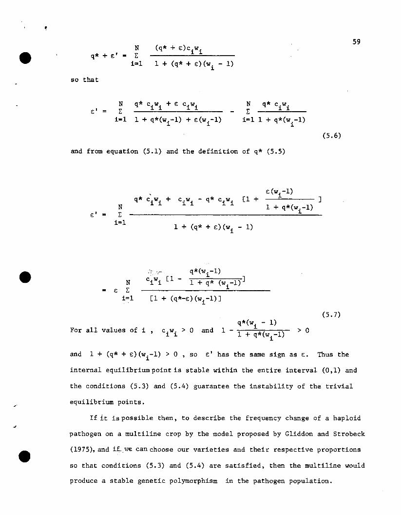
Nq* + e:' = 1:

i=l

so that

1 + (q* + e:)(wi - 1)

59

e:' =N q* ciwi + e: ciwi1:

i=l 1 + q*(wi -1) + e:(wi -1)

N q* c.w.1: ~ ~

i=l 1 + q*(w.-1)~

(5.6)

and from equation (5.1) and the definition of q* (5.5)

E' =N1:

i=l1 + (q* + E) (Wi - 1)

e: (wi-1)-....;;;;...---]

1 + q*(wi -1)

N= e: 1:

i=l [1 + (q*-e:)(wi -1)]

For all values of i ,q*(w. - 1)

c.w. > 0 and 1 - ~*( )~ ~ 1 + q w.-1

1

> 0

(5.7)

and 1 + (q* + e:)(w.-1) > 0 ,SO E' has the same sign as E. Thus the~

internal equilibrium point is stable within the entire interval (0,1) and

the conditions (5.3) and (5.4) guarantee the instability of the trivial

equilibrium points.

If it ispossible then, to describe the frequency change of a haploid

pathogen on a multiline crop by the model proposed by Gliddon and Strobeck

(1975), and iL.we can choose our varieties and their respective proportions

so that conditions (5.3) and (5.4) are satisfied, then the multiline would

produce a stable genetic polymorphism in the pathogen population.

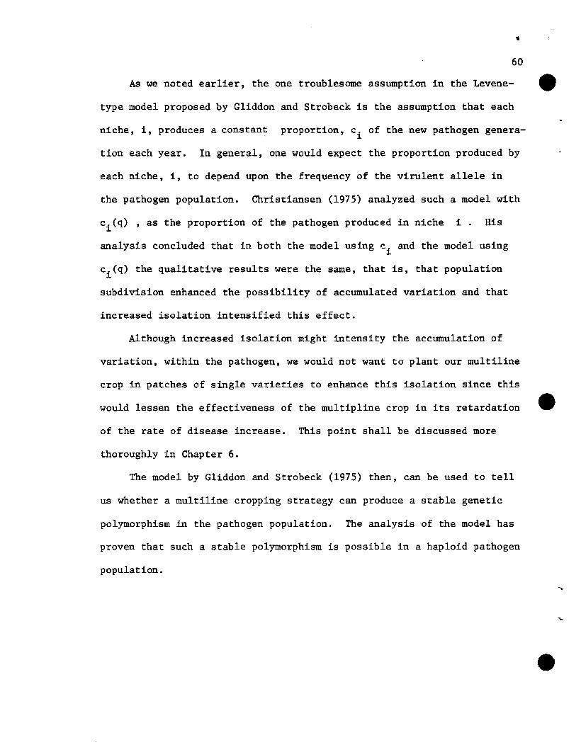
60

As we noted earlier, the one troublesome assumption in the Levene- ~

type model proposed by G1iddon and Strobeck is the assumption that each

niche, i, produces a constan~ proportion, c. of the new pathogen genera­1

tion each year. In general, one would expect the proportion produced by

each niche, i, to depend upon the frequency of the virulent allele in

the pathogen population. Christiansen (1975) analyzed such a model with

ci(q) , as the proportion of the pathogen produced in niche i. His

analysis concluded that in both the model using ci and the model using

ci(q) the qualitative results were the same, that is, that population

subdivision enhanced the possibility of accumulated variation and that

increased isolation intensified this effect.

Although increased isolation might intensity the accumulation of

variation, within the pathogen, we would not want to plant our multiline

crop in patches of single varieties to enhance this isolation since this

would lessen the effectiveness of the mu1tip1ine crop in its retardation

of the rate of disease increase. This point shall be discussed more

thoroughly in Chapter 6.

The model by G1iddon and Strobeck (1975) then, can be used to tell

us whether a multiline cropping strategy can produce a stable genetic

polymorphism in the pathogen population. The analysis of the model has

proven that such a stable polymorphism is possible in a haploid pathogen

population.

61

6. A MULTILINE MODEL FOR PATHOGEN POPULATION GROWTH.

The two models that we have looked at so far have studied the

change in gene frequencies of the pathogen and, in Leonard's model, the

change in gene frequencies of the host as well. Both models are useful

in determining whether it is possible that the genetic makeup of the

respective populations will at all maintain a polymorphic population and,

if so, for what parameter values this will hold. However, this is not

very helpful in determining the value of a particular cropping strategy.

Although a particular strategy, for rotating resistant varieties or for

a particular multiline crop may produce a stable set of frequenices for

the various races of the pathogen, the absolute numbers of the pathogen

attacking the crop could still be large enough to destroy the crop. Hence,

if we are interested in the effectiveness of a particular strategy, we

must be able to integrate the gene frequency models with some type of

population growth model.

Roughgarden (1979) has done some work along these lines. In his

studies of coevolution, he considered simultaneous equations of population

growth and of gene frequency change; however, in order to do any analysis

of these systems he had to assume that the gene frequencies were constant

and therefore, he studied only the equilibrium population sizes instead of

population growth. Barret (1978) did look at the multiline strategy from

the point of view of population growth, but then used his model to study

frequencies of the races and not to study the actual number of pathogens

produced. Also, Barret did not consider the amount of available tissue

as a limiting factor. Trenbath (1977) did attempt to consider available

tissue as a l~miting factor in his study of the growth of various races

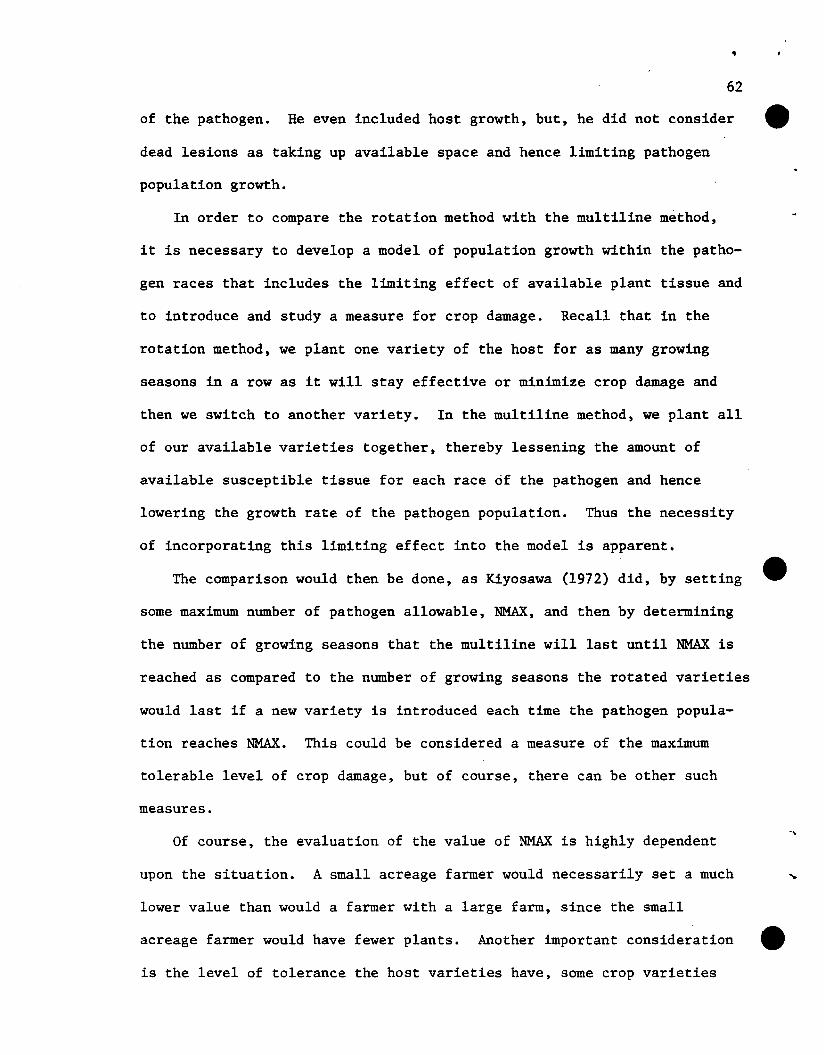
62

of the pathogen. He even included host growth, but, he did not consider

dead lesions as taking up available space and hence limiting pathogen

population growth.

In order to compare the rotation method with the multiline method,

it is necessary to develop a model of population growth within the patho­

gen races that includes the limiting effect of available plant tissue and

to introduce and study a measure for crop damage. Recall that in the

rotation method, we plant one variety of the host for as many growing

seasons in a row as it will stay effective or minimize crop damage and

then we switch to another variety. In the multiline method, we plant all

of our available varieties together, thereby lessening the amount of

available susceptible tissue for each race of the pathogen and hence

lowering the growth rate of the pathogen population. Thus the necessity

of incorporating this limiting effect into the model is appar~nt.

The comparison would then be done, as Kiyosawa (1972) did, by setting

some maximum number of pathogen allowable, NMAX, and then by determining

the number of growing seasons that the multiline will last until NMAX is

reached as compared to the number of growing seasons the rotated varieties

would last if a new variety is introduced each time the pathogen popula­

tion reaches NMAX. This could be considered a measure of the maximum

tolerable level of crop damage, but of course, there can be other such

measures.

Of course, the evaluation of the value of NMAX is highly dependent

upon the situation. A small acreage farmer would necessarily set a much

lower value than would a farmer with a large farm, since the small

acreage farmer would have fewer plants. Another important consideration ~

is the level of tolerance the host varieties have, some crop varieties

63

can support a relatively large number of lesions with little loss in

yield. Yield and other economic measures would also be important

considerations in determining a value for NMAX to use in the comparison

of a multiline cropping strategy with a rotation cropping strategy.

In order to make this comparison, we must first develop a new model

for population growth of the various pathogen races on the mixed host.

This general model for any number of host varieties could then be special­

ized to study the pathogen development on a single variety, as is used

in the rotation strategy.

The first question that needs to be addressed is just what are we

going to measure or count in our population growth model; do we want to

count spores or lesions? Since lesion number is more easily measured

and since lesions are the space occupying aspect of the pathogen, we

shall let Nij(t) be the number of lesions of race i on host variety j

at time t.

We shall, once again as in the previously discussed models, assume

that the pathogen develops in distinct generations and hence, we shall

use difference equations to model the growth of the pathogen population.

This assumption is not necessarily true, since some pathogen populations

are known to have multiple pathogen generations per growing season and

possibly overlapping generations. This model then, may be considered a

first attempt at comparing the multiline strategy with the rotation

strategy; since, although its assumptions may not be correct in all

instances, it is fairly intuitive and legitimate for some diseases.

Let the parameter, wij , be the number of possible new lesions left

to the next generation by an individual of pathogen race i on host

variety j , assuming that leaf area is not limiting. If we did not

64

assume that the pathogen is haploid and that like produces like, we

would need another subscript for wij to signify the type of new lesions

that are produced. If we then take the number of lesions of race i

on host variety j at generation t and multiply by wij , we will get the

total number of additional lesions left to generation t + 1 by pathogen

race i on host variety j.

The word "possible" in the above paragraph is important. The number

of new lesions of race i that are formed on host variety j in generation

t+l is limited by the amount of available or uninfected leaf area of

host variety j. The total number of possible lesions of race i produced

from lesions at time t on a sufficiently large field so that leaf area is

not limiting is:

This can be multiplied by the proportion of available leaf area of host ~

variety j to get Nij(t+l). As in the Levene type model described in the

previous chapter, we obviously assume random dispersal of new lesions and

this is a legitimate assumption since the host varieties are randomly

distributed.

The expression for the percentage of available leaf area of host

variety j is fairly complex and will therefore necessitate a stepwise

construction. First, we have the proportion of the field that is planted

Next, we must account for the proportion ofin host variety j to be c .•J

leaf area of host j that is uninfected at time t. We shall assume that the

amount of leaf area the host plant has is a constant and that the amount

of uninfected leaf area varies due to infection only. This is admittedly

a very simplistic assumption since the host does grow during the season,

65

but it could be acceptable if we consider a disease that only develops on

mature plants, where most of the growth has already occurred, we shall

denote the constant amount of leaf area that host variety j has if

planted throughout the field, in terms of the possible number of virulent

lesions as K This parameteris measured by taking the amount of leafj

area for the whole field planted with variety j and dividing it by the

size of the average virulent lesion on that host; this produces the

number of possible virulent lesions that could be supported on a field

of host j. Actually, K. is the number of possible virulent lesions thatJ

could be supported on an entire field of host j and is usually less than

the measurement of Kj calculated above. This is so since the number of

lesions are not necessarily closely packed.

Notice in describing K., we called it the number of possible virulentJ

lesions that could be supported on an entire field of host variety j. It

is quite apparent that, in many instances, the size of a lesion made by a

pathogen that is virulent on a specific host will be significantly larger

than the size of a lesion made by pathogen that is avirulent on that host.

Thus the size of each lesion of pathogen race i on host variety j can be

described by a measure re1ativeto the size of a virulent race j on host

variety j. The measure mij , for pathogen race i on host variety j

describes the relative size of the lesion and is therefore a number between

zero and one with mij = 1 Hence, if we have Nij(t) new lesions of

avirulent race i on host variety j at generation t, then the number of

virulent size lesion spaces that these lesions fill is mijNij(t).

Although we have assumed distinct generations so that only lesions

formed in the preceding generation live and reproduce, the dead lesions

66

of all the preceding generations in that growing season still remain on 4Itthe host and inhabit leaf area which cannot b-e:reinfected. Therefore, in

order to express the proportion ofnninfected leaf area of host j, we

need the number of lesions both living and dead that take up space on host

variety j at time t , namely:

Now, we can write the number of virulent lesion sized spaces that

have been filled up on host j by generation t as:

Hence the proportion of host j that have been infected up until generation

t can be expressed as follows:t

~ [(mij ) ~ Nij(k)]/(cjK.)i k=l J

All this allows us to write the following expression for the pro-

portion of originally available lesion spots on the whole field that is

still open and made available by variety j at time t:

tc.{l - ~ [(m

iJ.) ~ (k)]/[CjK

J,]}.

J i k=l

If we now multiply the total number of possible lesions of race i

produced from lesions at generation t by the percentage of uninfected

leaf area of host j that is available to these possible lesions of

race i in generation t+1, we get the number of new lesions of race i on

host variety j at generation t+1 as follows:

67

(6.1)

The above difference equation represents the growth of the pathogen

population during the growing season, but when Nij(t) is the last genera­

tion of pathogen before the crop is harvested, some type of overwintering

of the pathogen must occur and if needed in the measure of crop damage the

size of the crop would be measured. Thus if T is the number of genera-

tions the pathogen goes through in one growing season, then we reset the

time index as follows:

(6.2)

model.

Here, PH.. is the percentage of lesions of race i on host variety~J

j surviving over the winter. This is usually less than ten percent.

The equation (6.1) looks vaguely like the discrete pseudo-logistic

model, but does not suffer from the problems of the pseudo-logistic, such

as oscillation about the carrying capacity and the possibility of chaos

OMay, 1974). This is so because of the following extra parts to the

The parameter, cjKj' , is not the carrying capacity, but the amount

of available space and as such limits the number of new lesions that can

form on host variety j. That is, r(mi.)N . (t+1) must be limited soi J iJ

that:t+1

r (m •. )[ r N.. (k)J < c.K.i ~J k=l ~J J J

(6.3)

Hence, we need a third part to the model. That is, if (6.3) is

not true, then we must apportion the remaining uninfected leaf area on

host variety j proportionately to all pathogen races. The proportion of

uninfected leaf area assigned to each pathogen race i is computed to be

68

Nij(t+l)/ENij(t+l) where Nij(t+l) is the number of possible new lesions 4Iti

of pathogen race i on host variety j in generation t+l as given in

equation (6.1). Thus the number of virulent sized lesion spaces on

host variety j filled with pathogen race i at generation t+l is:

(6.4)

Although this appears to be the most equitable method for dividing

up the number of available spaces on host variety j among the different

races of new lesions, it does allow much empty space to exist after

the lesions have developed since the new lesions are not all as big as

the spaces (i.e., theavirulent lesions are smaller than the virulent

lesions). Nevertheless, since the new lesions all start at the same

size, it is legitimate to divide them up this way. Once this is done,

there is theoretically no more uninfected leaf area and thus this genera-

tion t+l must necessarily be the last generation for pathogen race i on

host variety j in the present growing session. Expression (6.4) is then

renamed Nij(T) and applied to equation (6.2) to determine the amount

surviving until the next growing season.

Since the model can at times require three different steps and since

step one, equation (6.1), is quite complex; the most practical method for

study of this model is through the use of computer simulation. This

simulation will be done for a single variety planting in a rotation type

of strategy and for a multiline cropping strategy.

Although most of the parameters may be fairly easily measured for

an individual field and host-pathogen system, we shall do a general ~

study of the two cropping models, and we shall leave any actual measure-

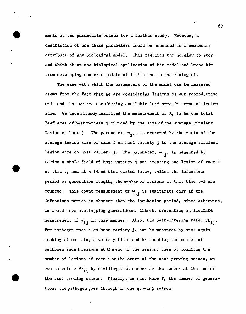
69

ments of the parametric values for a further study. However, a

description of how these parameters could be measured is a necessary

attribute of any biological model. This requires the modeler to stop'

and think about the biological application of his model and keeps him

from developing esoteric models of little use to the biologist.

The ease with which the parameters of the model can be measured

stems from the fact that we are considering lesions as our reproductive

unit and that we are considering available leaf area in terms of lesion

size. We have already described the measurement of Kj to be the total

leaf area of host variety j divided by the size of the average virulent

lesion on host j. The parameter, mij , is measured by the ratio of the

average lesion size of race i on host variety j to the average virulent

lesion size on host variety j. The parameter, wij ' is measured by

taking a whole field of host variety j and creating one lesion of race i

at time t, and at a fixed time period later, called the infectious

period or generation length, the number of lesions at that time t+l are

counted. This count measurement of wij is legitimate only if the

infectious period is shorter than the incubation period, since otherwise,

we would have overlapping generations, thereby preventing an accurate

measurement of wij in this manner. Also, the overwintering rate, PHij ,

for pathogen race i on host variety j, can be measured by once again

looking at our single variety field and by counting the number of

pathogen racei lesions at the end of the season; then by counting the

number of lesions of race i at the start of the next growing season, we

can calculate PH.. by dividing this number by the number at the end of1.J

the last growing season. Finally, we must know T, the number of genera-

tions the pathogen goes through in one growing season.

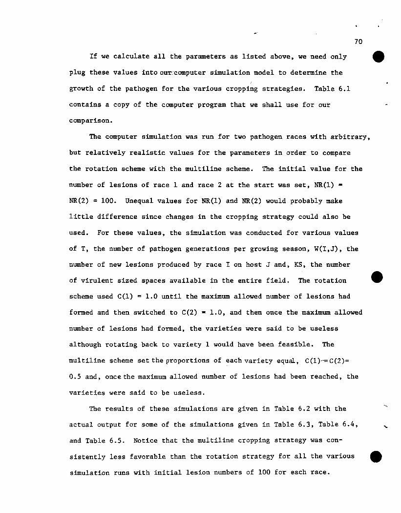
70

If we calculate all the parameters as listed above, we need only ~

plug these values into oU'r.·computer simulation model to determine the

growth of the pathogen for the various cropping strategies. Table 6.1

contains a copy of the computer program that we shall use for our

comparison.

The computer simulation was run for two pathogen races with arbitrary,

but relatively realistic values for the parameters in order to compare

the rotation scheme with the multiline scheme. The initial value for the

number of lesions of race 1 and race 2 at the start was set, NR(l) =

NR(2) = 100. Unequal values for NR(l) and NR(2) would probably make

little difference since changes in the cropping strategy could also be

used. For these values, the simulation was conducted for various values

of T, the number of pathogen generations per growing season, W(I,J), the

number of new lesions produced by race I on host J and, KS, the number

of virulent sized spaces available in the entire field. The rotation

scheme used C(l) = 1.0 until the maximum allowed number of lesions had

formed and then switched to C(2) = 1.0, and then once the maximum allowed

number of lesions had formed, the varieties were said to be useless

although rotating back to variety 1 would have been feasible. The

multiline scheme set the proportions of each variety equal, C(l)--=C(2)=

0.5 and, once the maximum allowed number of lesions had been reached, the

varieties were said to be useless.

The results of these simulations are given in Table 6.2 with the

actual output for some of the simulations given in Table 6.3, Table 6.4,

and Table 6.5. Notice that the multiline cropping strategy was con­

sistently less favorable than the rotation strategy for all the various

simulation runs with initial lesion numbers of 100 for each race.

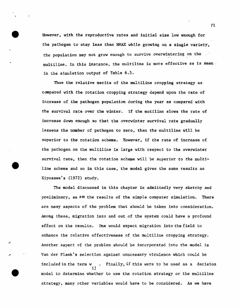
71

However, with the reproductive rates and initial size low enough for

the pathogen to stay less than NMAX while growing on a single variety,

the population may not grow enough to survive overwintering on the

multiline. In this instance, the multiline is more effective as °is seen

in the simulation output of Table 6.5.

Thus the relative merits of the multiline cropping strategy as

compared with the rotation cropping strategy depend upon the rate of

increase of the pathogen population during the year as compared with

the survival rate over the winter. If the mutiline slows the rate of

increase down enough so that the overwinter survival rate gradually

lessens the number of pathogen to zero, then the multiline will be

superior to the rotation scheme. However, if the rate of increase of

the pathogen on the multiline is large with respect to the overwinter

survival rate, then the rotation scheme will be superior to the multi-

line scheme and so in this case, the model gives the same results as

Kiyosawa's (1972) study.

The model discussed in this chapter is admittedly very sketchy and

preliminary, as aE the results of the simple computer simulation. There

are many aspects of the problem that should be taken into consideration.

Among these, migration into and out of the system could have a profound

effect on the results. One would expect migration into the field to

enhance the relative effectiveness of the multiline cropping strategy.

Another aspect of the problem should be incorporated into the model is

Van der Plank's selection against unncessary virulence which could be

decisionFinally, if this were to be used as aincluded in the term wij

model to determine whether to use the rotation strategy or the multiline

strategy, many other variables would have to be considered. As we have

72

mentioned in our discussion of the value of NMAX, both crop yield and

cost-effectiveness of the two cropping strategies would need to be

considered, as would any other economicaspect$ that would influence the

decision. The effect of the environment would also need to be considered

and would probably require the incorporation of a stochastic term into

model.

Thus there is much work to be done with this model. Since the

parameters of the model are fairly easy to measure and since its applica­

tion as a decision model could be of value, a further study of this model

should and will be conducted ina later work.

--

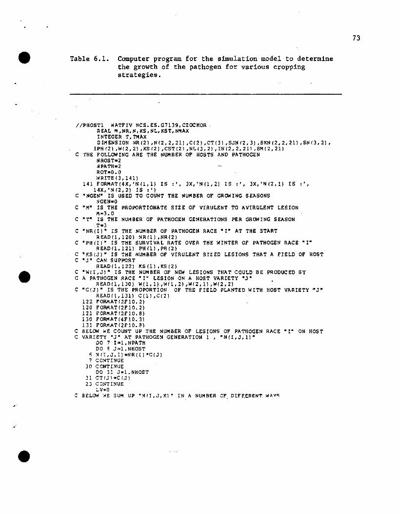
Table 6.1. Computer program for the simulation model to determinethe growth of the pathogen for various croppingstrategies.

//PHOSTI WATFIV NCS.ES.G7139,CZOCHOR .REAL M,NR,N,KS,NL,KST,NMAXINTEGER T, TMAXDIMENSION NR(2) ,N(2,2,21) ,C(2) ,CT(3) ,SJN/2,3) ,SKN(2,2,211 ,SN13,2),

1PH(2) ,W(2,2) ,KS/2) ,CST(2) ,NL(3,2) ,INC2,2,211 ,SM(2,21)C THE FOLLOWING ARE THE toIUMBER OF HOSTS AND PATHOGEN

NHOST-2~PATH-2

ROT-O.O\'iRITE(3,141)

141 FORMAT(4X,'N(1,1) IS :', 3X,'N(1,2) IS :', 3X,'N(2,1) IS :',14X, , N /2, 2) IS : t )

C "NGEN- IS USED TO COUNT THE NUMBER OF GROWING SEASONS)lGEN-O

C "M- IS THE PROPORTIONATE SIZE OF VIRULENT TO AVIRULENT LESION/11 ..3.0

C "T- IS THE NUMBER OF PATHOGEN GENERATIONS PER GROWING SEASONT-3

C "NR(I)" IS THE NUMBER OF PATHOGEN RACE uI- AT THE STARTREADC1,120) NR(1) ,NR(2)

C "PH(I)" IS THE SURVIVAL RATE OVER THE WINTER OF PATHOGEN RACE "I­READ C1 , 121) PH (1) , PH (2 )

C "KS(J)· IS THE NUMBER OF VIRULENT SIZED LESIONS THAT A FIELD OF HOSTC "J" CAN SUPPORT

READCl,122) KS(1) ,KS(2)C "W(I,J)- IS THE NUMBER OF NEW LESIONS THAT COULD BE PRODUCED BYC A PATHOGEN RACE "r n LESION ON A HOST VARIETY -J-

READC1,130) W(l, 1) ,W(1, 2) ,W(2, 1) ,W(2,2)C -C(J)" IS THE PROPORTION OF THE FIELD PLANTED wrTH HOST VARIETY ~J-

READ (1 , 131) C(1) , C(2)122 FORMAT/2F10.2)120 FORMAT(2F10.2)121 FORMAT/2F10.8)130 FORMAT(4F10.31131 FORMAT/2FIO.8)

C SELOW WE COUNT UP THE NUMBER OF LESIONS OF PATHOGEN RACE -r- ON HOSTC VARIETY nJ" AT PATHOGEN GENERATION 1 , -N(I,J,l)"

DO 7 I-l,NPATHDO ; J=l, NHOST

1'; )l /! , J , 1 ) -N R ( r ) ·C CJ )7 CON'l'INUE

30 CONTINUEDO 31 J-1, NHOST

31 CT (J I ..C (J)23 CONTINUE

LV-OC BELOW ~E SUM UP "NII,J,K)" IN A NUMBER OF. DtFF.ERENT WAV~

73

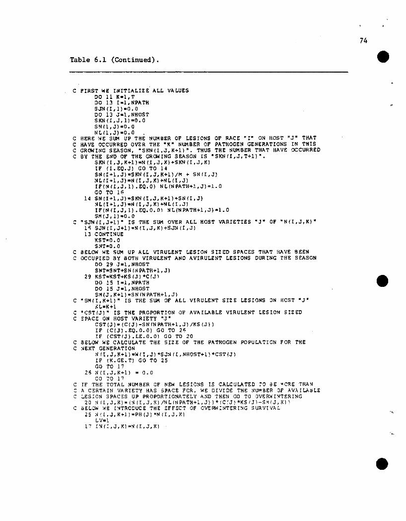
Table 6.1 (Continued).

C FIRST WE INITIALIZ E ALL VA roUESDO 11 K-l,T00 13 I-I, NPATHSJN (I, 1) -0. aDO 13 J-l,NHOSTSKN (I, J, 1)"0. aS NIl, J) -a •aNL (1, J) -0. a

C HERE ~"'E SUM UP THE NUMBER OF LESIONS OF RACE "I" ON HOST "J" THATC HAVE OCCURRED OVER THE 10K" NUMBER OF PATHOGEN GENERATIONS IN THISC GROWING SEASON, "SKN(I,J,K+l)". THUS THE NUMBER THAT HAVE OCCURREDC SY THE END OF THE GROWING SEASON IS "SKNII,J,T+l)".

SKN ( I , J , K+1 ) -N (I , J , K) +5 KN (I , J, K)IF (I.EQ.J) GO TO 14SN(I+l,J)-SKN(I,J,K+l)/M + SNII,J)NL(I+l,J)-N(I,J,K)+NL(I,J)IF(N (I,J, 1) .EO.O) NL(NPATH+l,J)-1. 0GO TO 16

14SN(I+l,J)-SKN(I,J,K+1)+SNII,J)~L(I+l,J)-NII,J,K)+NL(I,J)

IF (N (I , J, 1 ) • EO. O. 0 I ~ L (N PA TH+1 , J ) -I. 0SM (J , 1) -0.0

C "SJN(I,J+l)" IS '1'HE SUM OVER ALL HOST V1\RIETIES "J" OF "N(I,J,K)"1~ SJN(I,J+l)-NII,J,K)+SJN(I,J)13 CONTINUE

KST-O.OSNT-O. a

C BELOW WE SUM UP ALL VIRULENT ~ESION SIZED SPACES TH1\T HAVE BEENC OCCUPIED BY BOTH VIRULENT AND AVIRULENT r.ESIONS DURING 'rHE SEASON

DO 29 J-l, NHOSTSNT-SNT+SN (N PATH+l, J)

29 KST-KST+KSIJ)*C(JI00 15 I -1, NPATHDO 15 J-l,NHOSTS;<\ (J, K+l) -SN IN PATH+l, J)

C "SM(I,K+l)" IS THE SUM OF Ar.r. VIRULENT SIZE LESIONS ON HOST "J"KL-K+l

C "CST(J)" IS THE PROPORTION OF AVAILABLE VIRULENT r.ESION SIZEDC SPACE ON HOST VARIETY "J"

CST(J) - (C(J) -SN INPATH+1, J) /KS IJ) )IF (C(J).EO.O.O) GO TO 2~

IF (CSTIJ) .LE.O.O) GO TO 20C SHOW WE CAr.CULATE THE SIZ E OF THE PATHOGEN POPULATION FOR THEC ~EXT GENERATION

NfI,J,K+l)-W(I,J)*SJNfI,NHOST+l)*CST(J)IF IK.GE.T) GO TO 25GO TO Ii

26 NfI,J,K+l) - 0.0GO 1'0 Ii

C IF THE TOTAr. NUMBER OF NEW r.ESICNS IS CAr.CULATED TO dE ~C~E TPANC A CERTAIN VARIETY HAS SPACE FeR, WE DIVIDE THE NUMBER OF AV~ILA8LE

_ LESION SPACES UP PROPORTIONATELY AND '1'HEN GO TO OVER'~INTERING

20 :-I fI, J, K) .. (;.I (I, J, K) IN L (N PATH+l ,J) ) '" fC (J) "'KS (J 1-S,.,\ (J , K) ,C aELCW 'NE I~TRODUCE THE EFFECT OF OVERWINTERING SURIJtVAL

25 :-lrL,J,K+l)sPH(Jl*NCI,J,Klr.V-l

1 7 IN ( I , J, K) ,.~ I I , J, K)

74

--

..

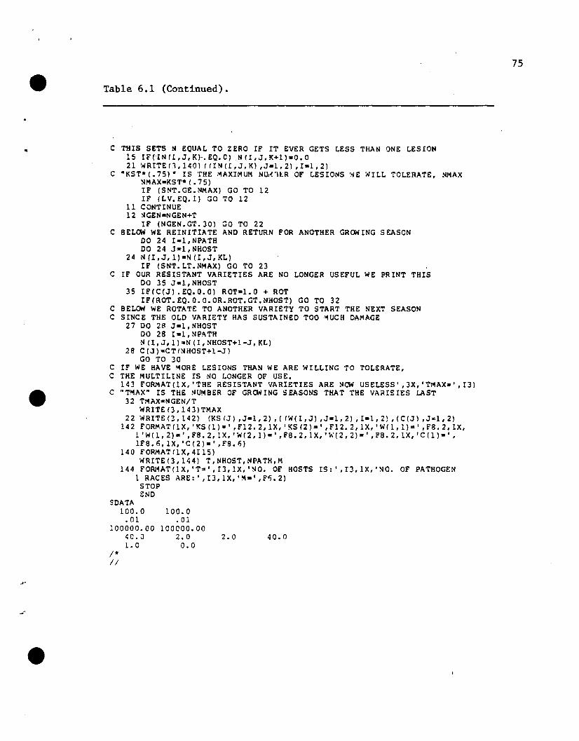
Table 6.1 (Continued).

C THIS SETS N EQUAL TO ZERO IF IT EVER GETS LESS THAN ONE LESION15 IF("IN(l,J,KhEQ.O) N(!,J,I<+l)-O.O21 't'lRITED,1401 IIIN(I,J,K) ,J-l,2) ,1-1,2)

C "KST* (.75)" IS THE ~AXIMUM NUiOt.R OF LESIONS ~'iE "'ILL TOLERATE, NMAXNMAX-KST* (.75)IF (SNT.GE.NMAX) GO TO 12IF (LV.EQ.l) GO TO 12

11 CONTINUE12 NGEN-NGEN+T

IF (NGEN.GT.30) GO TO 22C BELOW WE REINITIATE AND RETURN FOR ANOTHER GROWING SEASON

DO 24 I-I, NPATHDO 24 J-1, NHOST

24 N(I,J,l)-N(I,J,KL)IF (SNT.LT.NMAX) GO TO 23

C IF OUR RESISTANT VARIETIES ARE NO LONGER USEFUL WE PRINT THISDO 35 J-l,NHOST

35 IF(C(J) .EO.O.O) ROT-l.O + ROTIF(ROT.EO.O.O.OR.ROT.GT.NHOST) GO TO 32

C BELOW WE ROTATE TO ANOTHER VARIETY TO START THE NEXT SEASONC SINCE THE OLD VARIETY HAS SUSTAINED TOO ''1UCH DAMAGE

27 DO 28 J-l,NHOSTDO 28 I.l,NP.~TH

N(I,J,1)-N(I,NHOST+1-J,KL)28 C(J).CTINHOST+I-J)

GO TO 30C IF WE HAVE MORE LESIONS THAN WE ARE WILLING TO TOLERATE,C THE MULTILINE IS NO LONGER OF USE. '

143 FORJ'1AT(lX,'THE RESISTANT VARIETIES ARE NOW USELESS',3X','TI'\AXa:',I31C "TMAX" IS THE NUMBER OF GROWING SEASONS THAT THE VARIEIES LAST

32 TI'\AX-NGEN/TWRITE (3, l43)TMAX

22 't'lRITE(3,l42) (KSIJ) ,J-l,2),( IW(I,J) ,J-l,2) ,1-1,2) ,(C(J) ,Ja:l,2)142 FORMAT 11 X, 'KS (1)" • , F12. 2, IX, , KS (2)" I , F12. 2, IX, •W( 1 , l)" • , Fa. 2, IX,

1 'W (1,2) - ' , F8. 2, 1X, I W(2, 1) - I , Fa. 2, 1X, 'w (2, 2)" • , Fa. 2, IX, •C(1). I ,

lF8.n,lX,'C(2)·' ,F8.6)140 FO~~AT(lX,4115)

WRITE(3,144) T,NHOST,NPATH,M144 FORMATIIX,'T-',I3,lX,'NO. OF HOSTS IS:' ,I3,lX,'NO. OF PATHOGEN

1 RACES ARE:' ,I3,lX,'M.',F~.2)STOPEND

75

SDATA100.0

.01100000.00

40.J1.0

1*II

100.0.01

100000.002.00.0

2.0 40.0

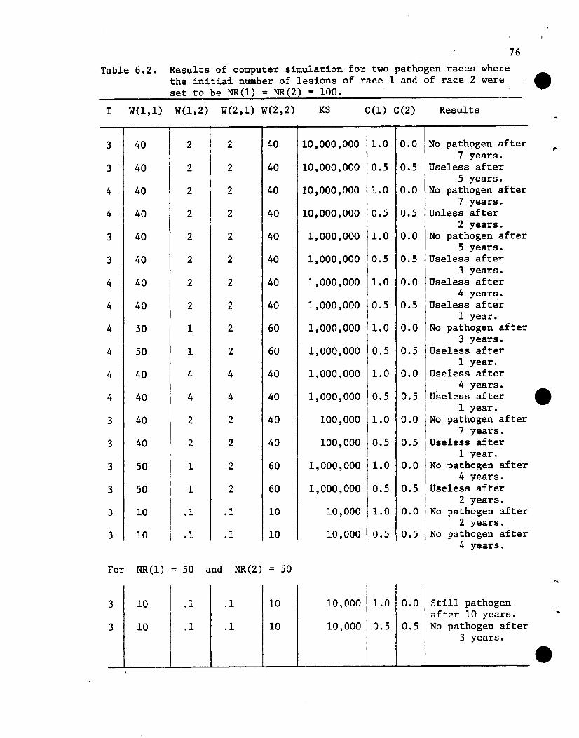
76

Table 6.2. Results of computer simulation for two pathogen races wherethe initiai number of lesions of race 1 and of race 2 were ~set to be NR(l) = NR(2) = 100.

T W(l,l) W(1,2) W(2,1) W(2,2) KS C(l) C(2) Results

4 years.

3 40 2 2 40 10,000,000 1.0 0.0 No pathogen after7 years.

3 40 2 2 40 10,000,000 0.5 0.5 Useless after5 years.

4 40 2 2 40 10,000,000 1.0 0.0 No pathogen after7 years.

4 40 2 2 40 10,000,000 0.5 0.5 Unless after2 years.

3 40 2 2 40 1,000,000 1.0 0.0 No pathogen after5 years.

3 40 2 2 40 1,000,000 0.5 0.5 Useless after3 years.

4 40 2 2 40 1,000,000 1.0 0.0 Useless after4 years.

4 40 2 2 40 1,000,000 0.5 0.5 Useless after1 year.

4 50 1 2 60 1,000,000 1.0 0.0 No pathogen after3 years.

4 50 1 2 60 1,000,000 0.5 0.5 Useless after1 year.

4 40 4 4 40 1,000,000 1.0 0.0 Useless after4 years.

4 40 4 4 40 1,000,000 0.5 0.5 Useless after1 year.

3 40 2 2 40 100,000 1.0 0.0 No pathogen after7 years.

3 40 2 2 40 100,000 0.5 0.5 Useless after1 year.

3 50 1 2 60 1,000,000 1.0 0.0 No pathogen after4 years.

3 50 1 2 60 1,000,000 0.5 0.5 Useless after2 years.

3 10 .1 .1 10 10,000 1.0 0.0 No pathogen after2 years.

3 10 .1 .1 10 10,000 0.5 0.5 No pathogen after

For NR(l) = 50 and NR(2) = 50

3 10 .1 .1 10 10,000 1.0 0.0 Still pathogenafter 10 years.

3 10 .1 .1 10 10,000 0.5 0.5 No pathogen after3 years.

"-

Table 6.3. Number of lesions from the simulation forKS(l) = KS(2) = 10,000,000, W(l,l) = W(2,2) = 40,W(1,2) = W(2,1) = 2, and T = 4.

Rotation from host variety 1 to host variety 2 after NMAX has beenreached.

N(l,l) is: N(1,2) is N(2,1) is N(2,2) is

100 0 100 03999 0 199 0

159930 0 399 06292139 0 786 0

62921 0 7 02501018 0 15 07436052 0 2 0

0 74360 0 00 148352 0 00 294501 0 00 578849 0 00 5788 0 00 11574 0 00 23136 0 00 46209 0 00 462 0 00 924 0 00 1848 0 00 3696 0 00 36 0 00 73 0 00 147 0 00 295 0 00 2 0 00 5 0 00 11 0 00 23 0 00 0 0 00 0 0 00 0 0 00 0 0 0

J"Multiline with 50% of the field planted in host variety 1, and50% in host variety 2.

N(l,l) is: N(1,2) is : N(2,1) is : N(2,2) is :--50 50 50 50 ...

1999 99 99 199941981 2099 2099 41981

77

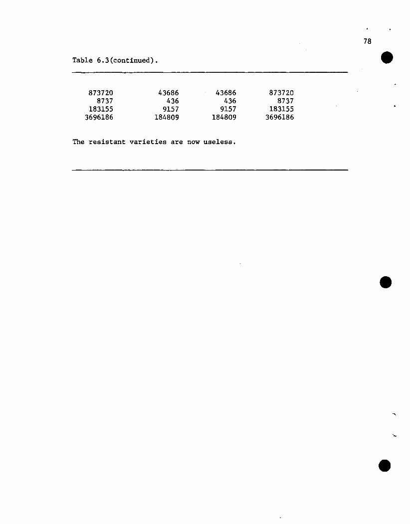
Table 6.3(continued).

78

8737208737

1831553696186

43686436

9157184809

43686436

9157184809

8737208737

1831553696186

The resistant varieties are now useless.

--

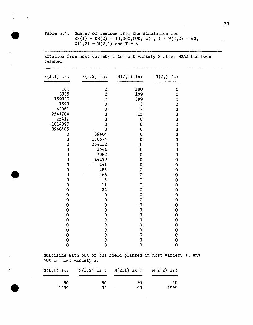
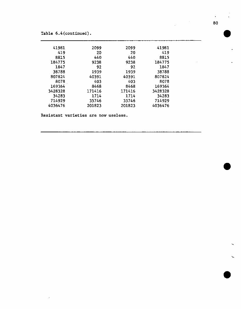
Table 6.4(continued).

80

41981419

8815184775

184738788

8078248078

1693643428328

34283714929

4036476

209920

4409238

921939

40391403

8468171416

171435746

201823

209920

4409238

921939

40391403

8468171416

171435746

201823

41981419

8815184775

184738788

8078248078

1693643428328

34283714929

4036476

Resistant varieties are now useless.

"-

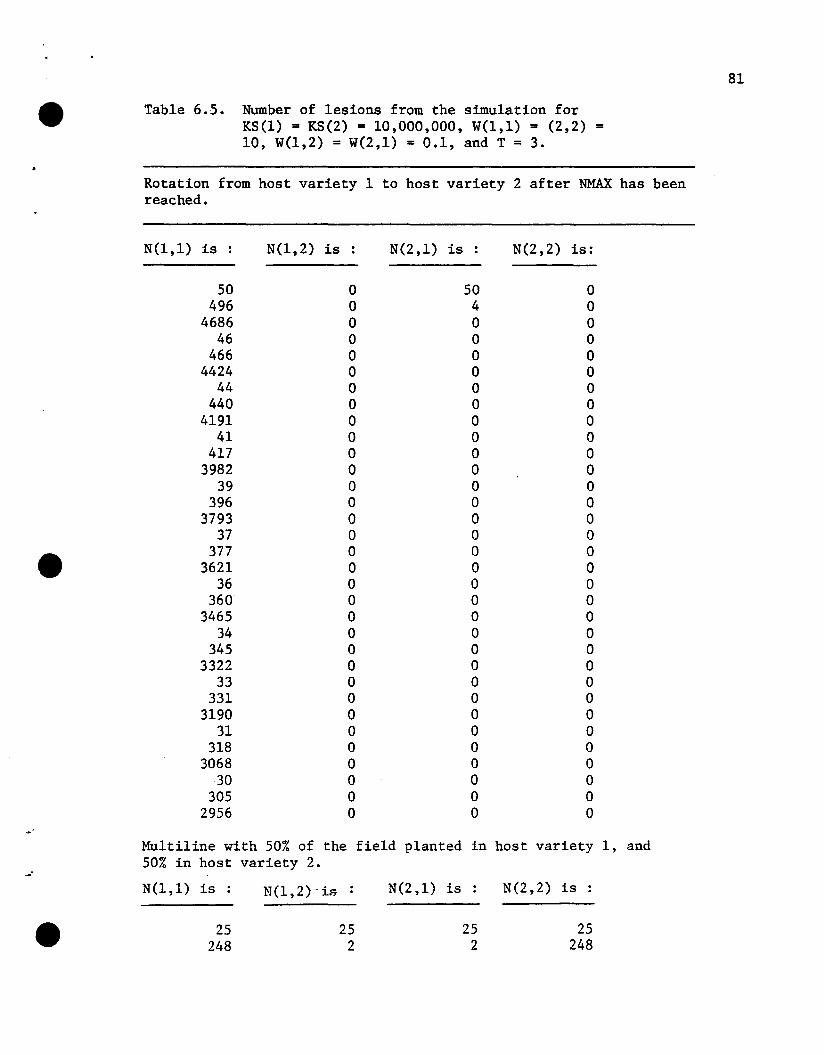
81

Table 6.5. Number of lesions from the simulation forKS(l) = KS(2) = 10,000,000, W(l,l) = (2,2) =10, W(1,2) = W(2,1) = 0.1, and T = 3.

Rotation from host variety 1 to host variety 2 after NMAX has beenreached.

N(l,l) is N(1,2) is N(2,1) is N(2,2) is:

50 0 50 0496 0 4 0

4686 0 0 046 0 0 0

466 0 0 04424 0 0 0

44 0 0 0440 0 0 0

4191 0 0 041 0 0 0

417 0 0 03982 0 0 0

39 0 0 0396 0 0 0

3793 0 0 037 0 0 0

377 0 0 03621 0 0 0

36 0 0 0360 0 0 0

3465 0 0 034 0 0 0

345 0 0 03322 0 0 0

33 0 0 0331 0 0 0

3190 0 0 031 0 0 0

318 0 0 03068 0 0 0

30 0 0 0305 0 0 0

2956 0 0 0~

Multiline with 50% of the field planted in host variety 1, and50% in host variety 2.

-"N(l,l) is : N(1,2)-is : N(2,1) is N(2,2) is :

25 25 25 25248 2 2 248

82

Table 6.5 (continued). e1183 11 11 1183

11 0 0 1150 0 0 59

293 0 0 2932 0 0 2

14 0 0 1473 0 0 73

0 0 0 00 0 0 0

'-

,-

83

7. CONCLUSION.

In the previous chapters, we have attempted to study a question

of paramount importance to modern agriculture. We have used mathe­

matical models to analyze how best to deploy the available cu1tivars

of a crop to prolong their cumulative resistance to plant pathogens.

In order to study this question, an explanation of what was happening

in the natural coevolution of a gene-for-gene system was needed. Van

der Plank (1963) provided such an explanation with his concept of

"stabilizing selection" or selection against unnecessary virulence and

against unnecessary resistance.

A number of mathematical models had been developed to study the

development of the pathogen races in a gene-for-gene system. Leonard

(1977) deve1oped~~mode1 for the express purpose of studying Van der

Plank's concept and analyzing if it was a viable exp1anaticn of what was

happening in the natural coevo1utionofa gene-for-gene system. The

development of this model and the preliminary attempts at analysis of

it were discussed in Chapter 3. We discovered that Leonard's (1977)

model did not adequately model the biological relationship that

Leonard had had in mind. The fact that the pathogen population changed

its genetic composition with each generation during the growing season

and in turn the host population changed its genetic composition as a

result of the genetic composition of the pathogen at the end of the

growing season, led to the sequential type of model proposed in Chapter

3. This new model produced inconclusive results for the linear

stability analysis of the internal singular point, but computer simula­

tions supported the existence of either a locally stable spiral point

84

or stable limit cycles. In either case, a polymorphism in both the ~

pathogen population and the host population would be preserved.

Nevertheless, when a so-called analogous continuous time model

was proposed by Fleming (1980) and shown to produce a center, an

analytic technique "waY; needed to show that the discrete time model of

Leonard (1977) was not as easily analyzed as the so-called continuous

time analog and that in fact it did not produce a center. Such a

technique was developed by adapting a method for discerning a center

from a focus that Poincare (1885) had developed for continuous time

systems. We have also discussed why this technique was one of the

relatively few techniques developed for continuous time systems that

was applicable to discrete time ~ystems.

The results of the long and arduous calculations required for

the applicationot this new method for difference equations were in one

respect, inconclusive. A completely general analytic result was not

feasible since it was necessary to describe what portions of the space

would produce either a positive or negative value for a sum of over

two hundred terms. The expression was therefore calculated for

various values of the parameters by using a computer. In all such

cases, except for those where a biologically stable polymorphism was not

probable, it was shown that the internal equilibrium point was a stable

focus and not a center. Thus it appeared that Van der Plank's concept

of "stabilizing selection" is a viable explanation of what was

happening in the natural coevolution of a gene-for-gene host-pathogen

system.

The only disturbing aspect of this analysis was that we had once

again resorted to the computer and had apparently gained relatively

"-

85

little, in this instance, from this new technique. It did, however,

bring up a questionof increasingly greater importance in the analysis

of models of biological systems. That is, when should any attempt at

an analytic answer be given up in favor of a numerical result? Had

we needlessly wasted time seeking an analytical result? These questions

should always be kept in mind whenever studying any model. The

benefits, in terms of a general result, to be gained must be weighed

against the cost, in terms of effort and time, of gaining an analytical

result. We had originally decided that since the preliminary linear

analysis was inconclusive and the numerical analysis did allow a

conclusion, then an attempt at any further analysis was too costly.

However, when Fleming (1980) published his so-called analog, the

possible benefits of an analytic result were heightened until they

outweighed the cost; that is, until it became necessary to analyze

an expression with an discouragingly large number of terms. Thus,

in our opinion, the decision of whether to do an analytical or

numerical analysis, depends entirely on a cost-benefit analysis of

the question.

Once we had studied this model of the coevolution in nature of a

gene-for-gene host-pathogen system, we needed to study the genetic

evolution of a pathogen population on a mixed host. Only then could

we develop a model to compare the relative merits of a multi-line

cropping system with a single variety, pure line cropping system. To

this end, the classic model of Levene (1953) for a multiple niche

polymorphism and its analog for haploids by Gliddon and Strobeck

(1972) were studied. The applicability of the Glidden and Strobeck

model to the evolution of the pathogen on the multiline crop was

86

discussed and a stability analysis of its internal equilibrium was

conducted. It was concluded that a multiline cropping system could

produce a stable polymorphism in the pathogen population or in other

words, that a stable internal equilibrium point for gene frequencies

was possible.

Although this model showed that a multipline crop could be used

to stabilize gene frequencies at some internal equilibrium point, it

told us relatively little about its effectiveness in terms of slowing

down or stopping an epidemic. The fact that gene frequencies were

stabilized is inconsequential if the pathogen number is increasing

rapidly and ends up infecting a large part of the crop. Thus, in

order to compare the effectiveness of a multiline crop with the

effectiveness of a single variety monoculture that is changed each

time the resistance breaks down, it was necessary to develop a model

to analyze effectiveness. It was decided that a variety would

remain effective until a certain maximum number of lesions were on

that variety. Thus instead of using yield or some other quality to

measure the loss in,\effectiveness, we used lesion number and thus

developed a model that counted lesion number.

The model was simply a population growth model with the number

of new lesions being limited by the available or uninfected plant

leaf area. The model was analyzed by computer simulation because

of its complexity. It was discovered that in almost all instances,

a single variety monoculture, that is replaced each time an unacceptable

number of lesions occur, is more effective at prolonging the

cumulative lifetime of the varieties than is a multiline made up of

the same varieties. The only time a multiline crop seems to be

better is when it slows down the rate of increase of the pathogen

enough so that the pathogen cannot overcome the overwintering rate.

Thus, if the overwintering rate is very low, the multiline

crop may slow the pathogen reproduction enough so that it cannot

recover and. hence the pathogen would be eradicated. Of course, these

results were contingent on the assumptions made in the model.

87

APPENDICES

88

"-

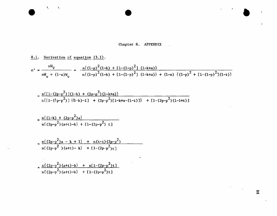
e\. .., -

Chapter 8. APPENDIX

•

8.1. Derivation ££ equation ~.

n' = nWV---nW + (l-n)Wv v

=2 2n{(l-p) (l-k) + [l-(l-p) ] (l-k+a)}2 2 2 2}n{(l-p) (l-k) + [l-(l-p) ] (l-k+a)} + (l-n) {(l-p) + [l-(l-p) ](l-t)

2 2}n{[1-(2p-p )](l-k) + (2p-p )(l-k+a)- 2 2 2

n{[1-(2p-p )] [Q-k)-l] + (2p-p )[l-k+a-(l-t)]} + [1-(2p-p )(l-l+t)]

2_ n{(l-k) + (2p-p )a}- 2 2

n{(2p-p )(a+t)-k} + [1-(2p-p ) t]

2 2_ n{(2p-p )a - k + I} + n(t-t)(2p-p)- 2 2

n{(2p-p ) (a+t)- k} + [1-(2p-p )t]

2 2_ n{(2p-p )(a+t)-k} + n[1-(2p-p )t]- 2 2

n{(2p-p )(a+t)-k} + [1-(2p-p )t]

00\0

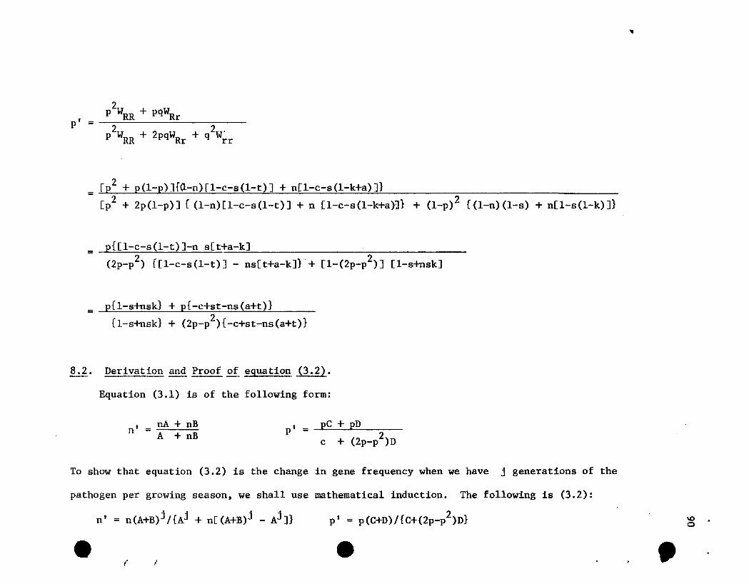
2P WRR + pqWRrp' = ------------p2WRR + 2pqW

R+ q2w.

r rr

_ [p2 + p(l-p)]{a-n)[l-c-s(l-t)] + n[l-c-s(l-k+a)]}- 2 } 2[p + 2p(1-p)] {(l-n)[l-c-s(l-t)] + n [l-c-s(l-k+a)l + (l-p) {(l-n)(l-s) + n[l-s(l-k)]}

_ p{[l-c-s(l-t)]-n s[t+a-k]- 2 } 2(2p-p ) {[l-c-s(l-t)] - ns[t+a-k] + [1-(2p-p )] [l-s+nsk]

= p{l-s+nsk} + p{-c+st-ns(a+t)}2{l-s+nsk} + (2p-p ){-c+st-ns(a+t)}

8.2. Derivation and Proof of equation (3.2).

Equation (3.1) is of the following form:

..

, _ nA + nBn - A + nB

p' = pC + pD 2c + (2p-p )D

To show that equation (3.2) is the change in gene frequency when we have j generations of the

pathogen per growing season, we shall use mathematical induction. The following is (3.2):

n' = n(A+B)j/{Aj + n[(A+B)j - Aj ]}

e"

I

p' = p(C+D)/{C+(2p-p2)D}

e •\0 •o

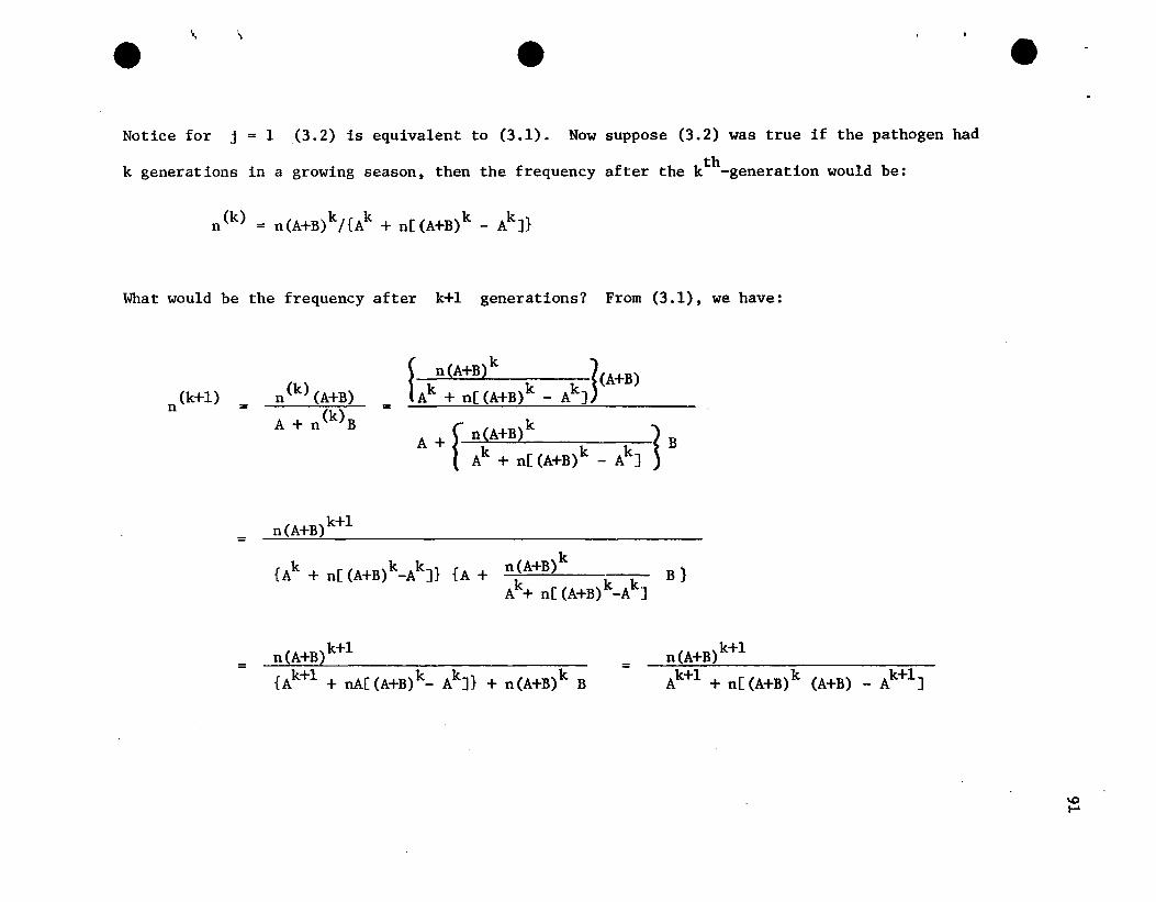
e \, " e e

Notice for j = 1 (3.2) is equivalent to (3.1). Now suppose (3.2) was true if the pathogen had

k generations in a growing season, then the frequency after the kth-generation would be:

n(k) = n(A+B)k/{Ak + n[(A+B)k _ Ak]}

What would be the frequency after k+l generations? From (3.1), we have:

(k+l)n =

=

n(k) (A+B)

A + n(k)B

n(A+B)k+l

=f

k Jn(A+B) (A+B)Ak + n[(A+B)k _ Ak]

f k 1A + n(A+B) BAk + n[(A+B)k _ Ak]

k{Ak + n[ (A+B)k_Ak]} {A + n(A+B) B}

Ak+ n[(A+B)k_Ak]

=n(A+B)k+l

{Ak+l + nA[(A+B)k- Ak]} + n(A+B)k B=

n(A+B)k+l

Ak+l + n[(A+B)k (A+B) _ Ak+l ]

\DI-'

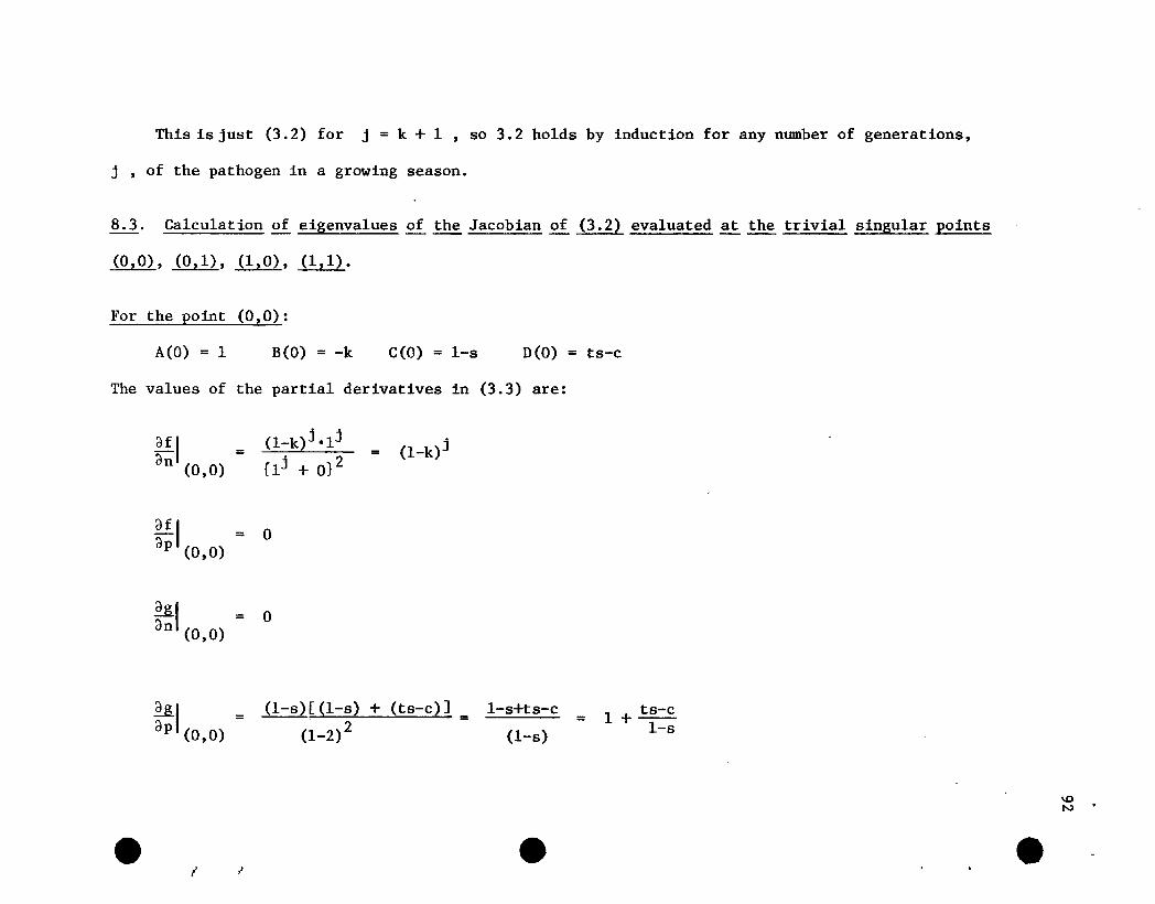
This is just (3.2) for j = k + 1 , so 3.2 holds by induction for any number of generations,

j , of the pathogen in a growing season.

8.3. Calculation of eigenvalues of the Jacobian of (3.2) evaluated at the trivial singular points

(0,0), (0,1), (1,0), (1,1).

For the point (0,0):

A(O) = 1 B(O) = -k C(O) = l-s D(O) = ts-c

The values of the partial derivatives in (3.3) are:

afl = (l-k)j elj= (l-k)j

an (0,0) {lj + 0}2

afl °ap (0,0) =

~I - °an (0,0) -

e

~I =ap (0,0)

I I

(l-s)~(l-s) + (ts-c)] = l-s+ts-c = 1 + ts-c(1-2)2 (l-s) l-s

e e\0N .

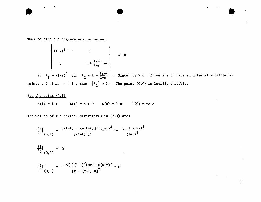
... '0,-Thus to find the eigenvalues, we solve:

(l-k)j - A °

e

= °

e

°So A = (l-k)j

1and

1 + ts-c1-s -A

A2

= 1 + ts-c1-s • Since ts > c , if we are to have an internal equilibrium

point, and since s < 1 , then IA21 > 1. The point (0,0) is locally unstable.

For the point (0,1)

A(l) = 1-t B(l) = a+t-k C(O) = l-s D(O) = ts-c

The values of the partial derivatives in (3.3) are:

af lan (0,1)

_ [(l-t) + (a+t-k)]j (l-t)j- [(1_t)j]2 =

(1 + a -k)j

(l-t)j

~I = °ap (0,1)

-s(l) (1-1)2[Dk + C(a+t)] = °[C + (2-1) D]2~·~f(O, 1) =

\0W

~

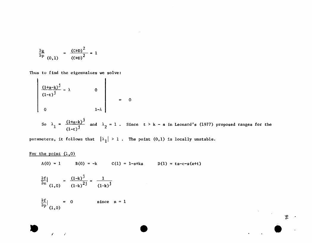
dP (0,1)

2(C+D) = 1

2(C+D)

Thus to find the eigenvalues we solve:

j0(l+a-k) _ A

(l-t)j

I = 0

1-1..0

So Al =j

(l+a-k) and 1..

2= 1 .

(l-t)jSince t > k - a in Leonard's (1977) proposed ranges for the

parameters, it follows that 11.. 1 1 > 1. The point (0,1) is locally unstable.

For the point (1,0)

A(O) = 1 B(O) = -k C(l) = l-s+ks D(l) = ts-c-s(a+t)

Eil = (l-k)j 1=dn (1,0) (l-k)2j (l-k)j

-dfl = 0dP (1,0)

,. "

since n = 1

- e\0.po.

e ~, " e e

E-B.I = °an (1,0)

since p = °

~Iap (1,0)

_ C(C+D)- C2

= l-s+ks+ts-c-s(a+t) = 1 _ c+sal-s+ks l-s+ks

Thus to find the eigenvalues we solve:

1

°--- A(l-k)j

I = °1 _ c+sa - A° l-s+ks

1So 1..1 = (l-k)j

locally unstable.

For the point (1,1)

and 1.. 2c+sa

= 1 - l-s+ks • Since k < 1 , then 11..1

1 > 1 . The point (1,0) is

A(l) = 1-t B(l) = a+t-k C(l) = l-s+ks D(l) = ts-c-s(a+t)

af lan (1,1)=

(A+B)j Aj

(A+B)2j=

Aj

(A+B)j \0\JI

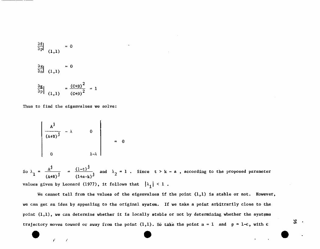
~ = 0dP (1,1)

~= 0

dn (1,1)

~I= (C+D)2 = 1

dP (1,1) (C+D) 2

Thus to find the eigenvalues we solve:

Aj

(A+B)j- A 0

I = 0

0 l-A

So A = Aj (l-t)jand A2 = 1 • Since t > k=1 (A+B)j (l+a-k)j

- a , according to the proposed parameter

values given by Leonard (1977), it follows that IAll < 1 •

We cannot tell from the values of the eigenvalues if the point (1,1) is stable or not. However,

we can get an idea by appealing to the original system. If we take a point arbitrarily close to the

point (1,1), we can determine whether it is locally stable or not by determining whether the syst~ms

trajectory moves toward or away from the point (1,1). So take-the point n = 1 and p = 1-£, with £

e,- I'

e e\00'

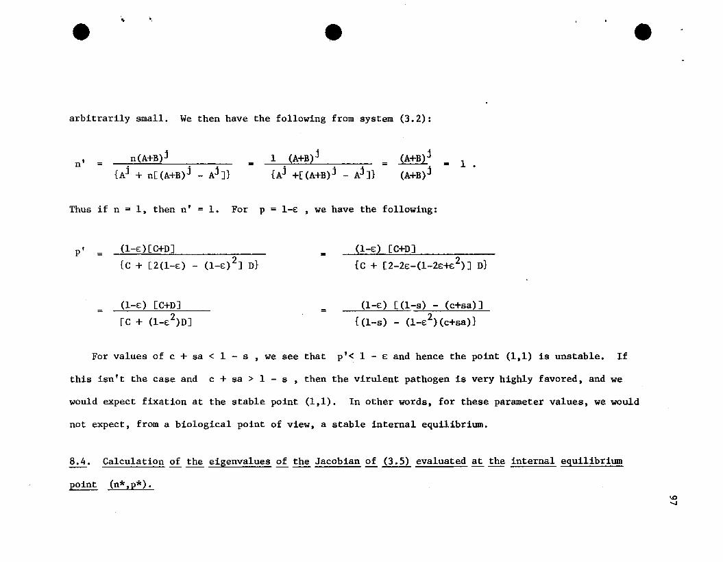
e \ '\ e e

arbitrarily small. We then have the following from system (3.2):

n' =n(A+B)j

{Aj + n[ (A+B)j - Aj ]}=

1 (A+B)j

{Aj +[(A+B)j - Aj ]}=

(A+B)j

(A+B)j= 1 .

Thus if n = 1, then n' = 1. For p = l-E , we have the following:

p' =

=

(l-E)[C+D]

{C + [2(1-E) - (1_E)2] D}

(l-E) [C+D]

[C + (l-E 2 )D]

=

=

(l-E) [C+D]

{C + [2-2E-(1-2E+E2)] D}

(l-E) [(l-s) - (c+sa)]

{(l-s) - (1-E2)(c+sa)}

For values of c + sa < 1 - s , we see that p'<l - E and hence the point (1,1) is unstable. If

this isn't the case and c + sa > 1 - s , then the virulent pathogen is very highly favored, and we

would expect fixation at the stable point (1,1). In other words, for these parameter values, we would

not expect, from a biological point of view, a stable internal equilibrium.

8.4. Calculation of the eigenvalues of the Jacobian of (3.5) evaluated at the internal equilibrium

point (n*,p*).\0".J

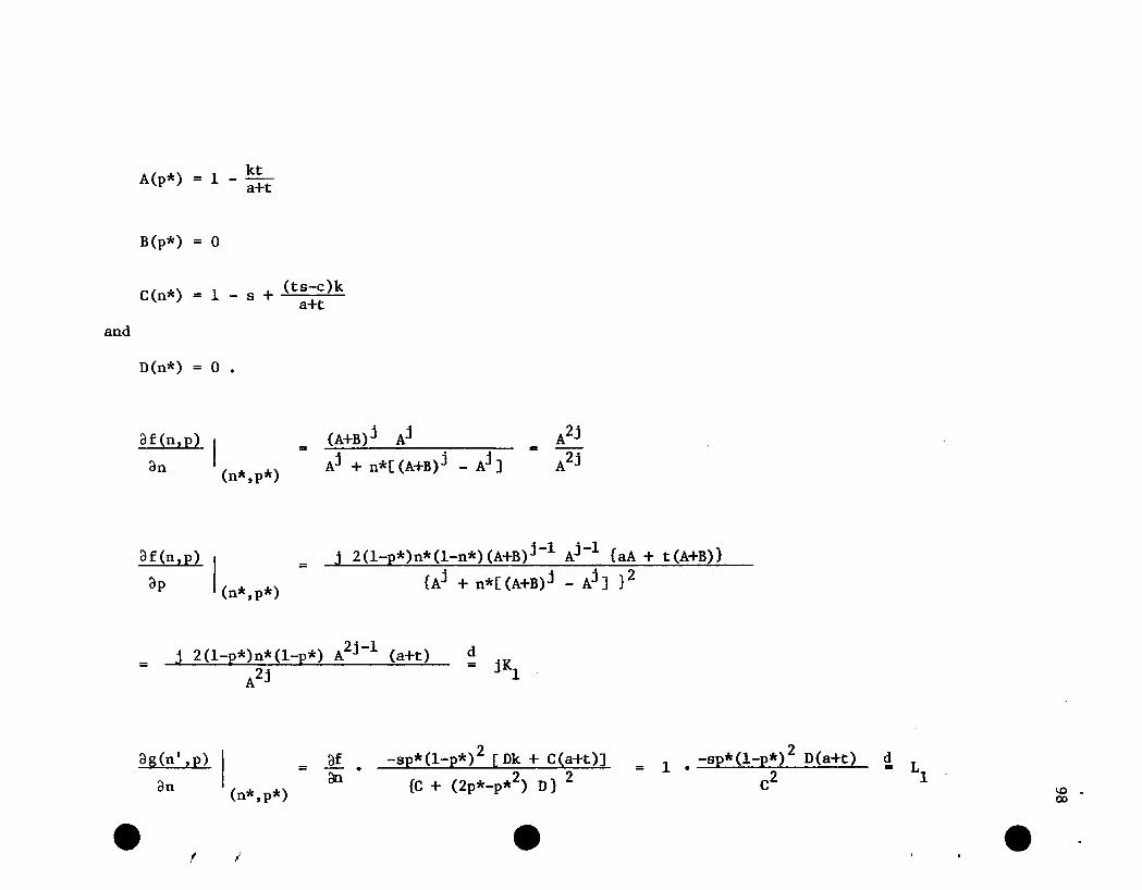
A(p*) = 1 _ kta+t

B(p*) = 0

C(n*) = 1 - s + (ts-c)ka+t

and

D(n*) = 0 •

af(n,p)

an I(n*,p*)

_ (A+B)j Aj

- Aj + n*[ (A+B)j - Aj ]=

A2j

A2j

af(n,p) Iap (n*,p*)

= j 2(1-p*)n*(1-n*)(A+B)j-l Aj -1 faA + t(A+B)}

{Aj + n*[ (A+B)j - Aj ] } 2

=2j-lj 2(1-p*)n*(1-p*) A (a+t)

A2j

d= jK

1

ag(n' ,p)

an

e!

I(n*,p*)

I

= afan-2-sp*(l-p*) [Ok + C(a+t)]

2 2{C + (2p*-p* ) D}

e

2= 1 _ -sp*(l-p*) D(a+t)

c2d L

1

e\0 •co

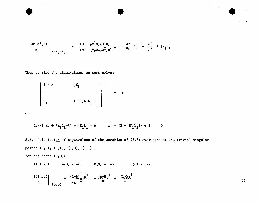
'." .e e e

ag(n' ,p)

ap I(n*,p*)

= (C + p*2D) (C+D) af+ - L{C + (2p*_p*2)D} 2 ap 1

_ c2- Z,+jK_L

C -1 1

Thus to find the eigenvalues, we must solve:

or

1 - A

Ll

jrs.

1 + jKlLl - A

= °

(I-A) (1 + jKlLl-A) - jKlLl = ° 2

A - (2 + jrs.Ll)A + 1 = °

8.5. Calculation of eigenvalues of the Jacobian of (3.5) evaluated at the trivial singular

points (0,0), (0,1), (1,0), (1,1) •

For the point (0,0):

A(O) = 1 B(O) = -k C(O) = l-s D(O) = ts-c

af(n,p)1

an (0,0)=

(A+B)j Aj

(Aj )2= (A1B) j =

(l-k)j1 \0

\0

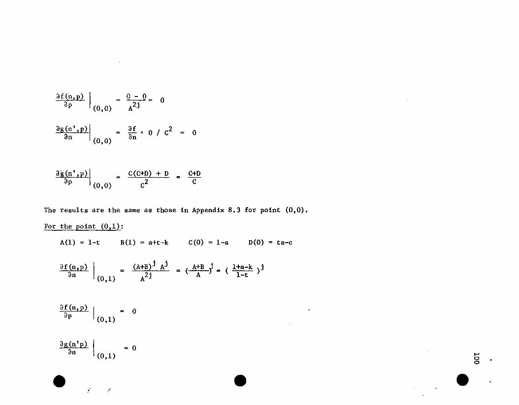
df(n,p) I °- 0 °= -=dP (0,0) A2j

ag(nl,p)1 = ~ · ° / c2 = °an (0,0) dn

ag(nl,p)1 = C(C+D) + D =

ap (0,0) c2C+D

C

The results are the same as those in Appendix 8.3 for point (0,0).

For the point (0,1):

A(l) = 1-t B(l) = a+t-k C(O) = 1-s D(O) = ts-c

af (n,p) I =

an (0,1)(A+B)j A

j= ( A+B r= ( l+a-k )j

A2j A 1-t

af(n,p) I =

°ap (0,1)

dg(n'p) I= °an (0,1) t-'

00

e e e. l

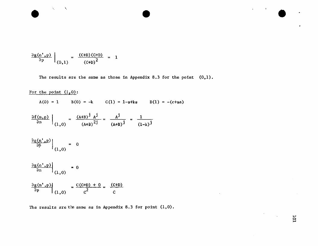
• \, e e

ag(nl,p) I =

ap (0,1)(C+D) (C+D)

(C+D) 2 = 1

The results are the same as those in Appendix 8.3 for the point (0,1).

For the point (1,0):

A(O) = 1 B(O) = -k C(l) = 1-s+ks D(l) = -(c+sa)

af (n,p) I = (A+B)j Aj Aj 1= =an (1,0) (A+B)2j (A+B)j (l-k)j

ag(nl,p)1ap = 0

(1,0)

ag(n I ,p)I = 0an (1,0)

aMC(C+D) + 0 (C+D)- -- -

ap (1,0) c2 C

The results are the same as in Appendix 8.3 for point (1,0).

I-'oI-'

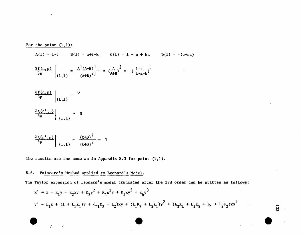
For the point (1,1):

A(l) = 1-t B(l) = a+t-k C(l) = 1 - s + ks D(l) = -(c+sa)

df (n,p)dn

_ Aj(A+B)j

(1,1) - (A+B)Zj

A j= (A+B) = (l-t j

, I _ 1_)

df(n,p) 0=dP (1,1)

ag(n',p)1 = 0an (1,1)

ag(n' ,p)Iap (1,1)

=Z

(C+D) = 1Z(C+D)

The results are the same as in Appendix 8.3 for point (1,1).

8.6. Poincare's Method Applied to Leonard's Model.

The Taylor expansion of Leonard's model truncated after the 3rd order can be written as follows:

, _ 2 Z 2 3x - x + K1y + KZxy + K3y + K4x y + KSxy + K6y

y' = L1x + (1 + L

1K

1)y + (L

1KZ + LZ)XY + (L1K3 + LZK1)YZ + (L3K1 + L1KS + L4 + LZK2)XYZ

• ,. e eI-'oI',.)

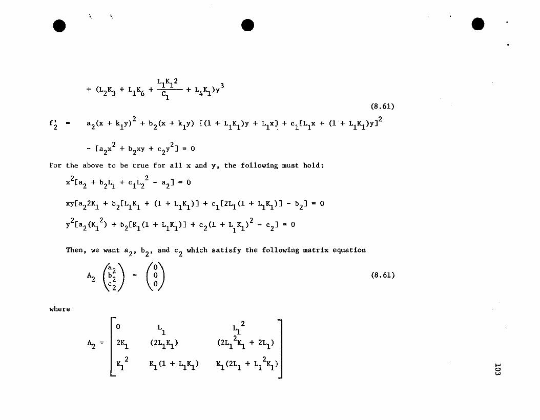
e " '. e e

fi =

Ll K12 3+ (L2K3 + Ll K6 + C + L4~)Y

1(8.61)

2 . 2a 2(x + kly) + b2(x + kly) [(1 + LlKl)y + Llx~ + Cl[Llx + (1 + LlKl)y]

2 2- [a2x + b2xy + c2y ] = 0

For the above to be true for all x and y, the following must hold:

2 2x [a2 + b2Ll + cl L2 - a 2] = 0

xy[a22~ + b2[Ll Kl + (1 + LlKl )] + cl [2Ll (1 + LlKl )] - bZ] = 0

2 2 2y [a2 (Kl ) + b2[Kl (1 + LlKl )] + c2(1 + LlKl ) - c2] = 0

Then, we want a 2, b2, and c2 which satisfy the following matrix equation

A2 (~O = 0)where

(8.61)

0 L L 21 1

A2 = I 2Kl (2Ll Kl ) (2L/~ + 2Ll )

~2 Kl(l + LlKl )2

Kl(ZLl + Ll Kl ) I .....0w

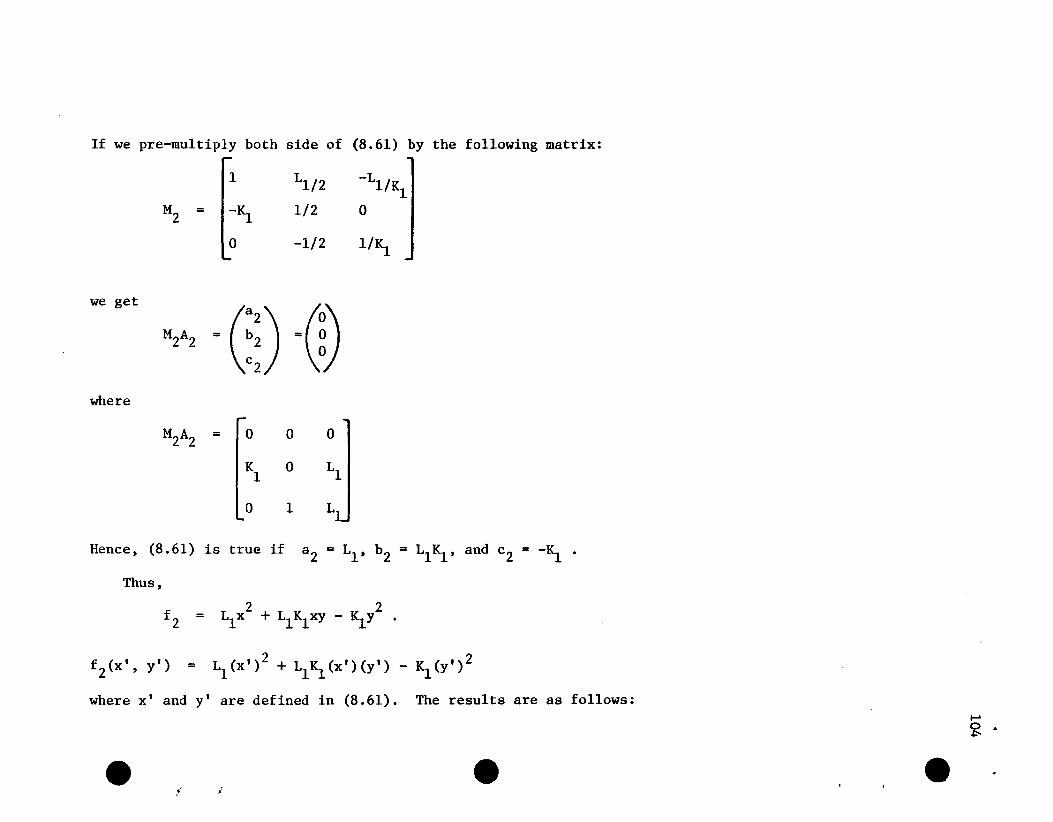
If we pre-multiply both side of (8.61) by the following matrix:. ,1 Ll/2 -Ll/K1

M2:::

I-Kl 1/2 0

0 -1/2 l/Kl

we get

=(:D =(DM2A2

where

M2A2::: fa 0 0

Kl

0 Ll

0 1 L

Hence, (8.61) is true if a2 ::: Ll , b2 ::: LlKl , and c2 ::: -~ •

Thus,

2 2f 2 ::: Llx + LlKlxy - Kly

f (x' y') ::: L (x,)2 + L K_ (x')(y') - K (y,)22' 1 l--r 1

where x' and y' are defined in (8.61). The results are as follows:

e ,,' /e e

I-'o ..po

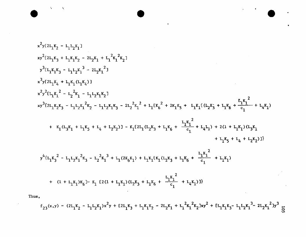
'" \e

2x y[2L1K2 - L1L2K1J

e ew

2 2 2xy [2L1K3 + L1K

1K2 - 2L2K1 + L1 K1 K2J

3 3 2Y [L1K1K3 - L1L2K1 - 2L2K1 J

3x y[2L1K4 + L1K1

(L1K4)J

2 2 2 2x Y [L1K1 - L2 K1 - L1L2K1K2]2

3 2 2 2 2 . L1K1xy {2L1K2K3 - L1L2~ K2 - L1L2K1K3 - 2L2 K1 + L1[K6 + 2K1KS + L1K1[(L2K3 + L1K6 + -c---1

+ L4~)

L1~2+ K1 (L3K1 + L1KS + L4 + L2K2)] - K1[2L1 (L2K3 + L1K6 + C + L4L1) + 2(1 + L1~)(L3~

1

+ L1KS + L4 + L2K2)]}

24 2 2 2 3 L1K1

Y {L1K3 - L1L2K1 K3 - L2 K1 + L1 (2K6K1) + L1K1[K1(L2K3 + L1K6 + c1

+ L1K1)

2L1K1+ (1 + L1K1)K

6J- K1 [2(1 + L1K1)(L2K3 + I'lK6 + c_ + L4K1)]}

Thus,

f 23 (x,y) 2 2 2 2 3. 2 3(2L1K2 - L1L2K1)x y + [2L1K3 + L1K1K2 - 2L2K1 + L1 ~ K2]xy + [L1~K3- L1L2~ - 2L2K1 ]Y b

\J1

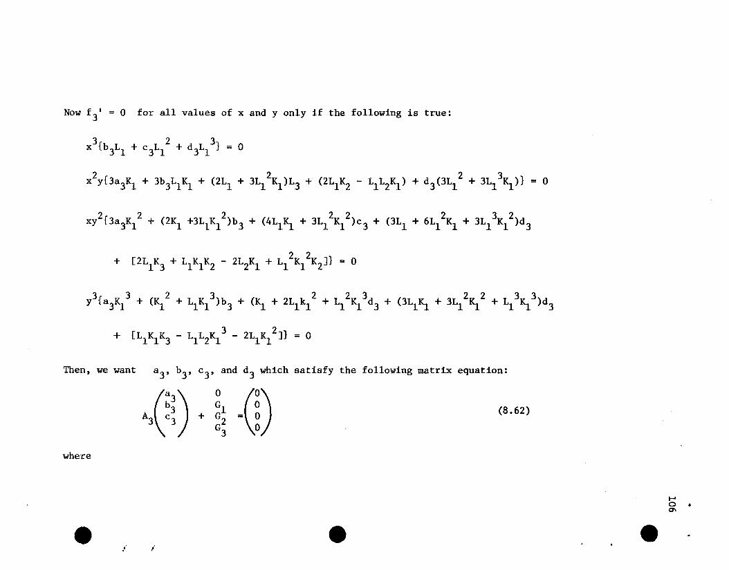
Now f 3 ' = 0 for all values of x and y only if the following is true:

3 2 3x {b3LI + c3LI + d3L

I} = 0

2 2 2 3x y{3a3KI + 3b3Ll Kl + (2LI + 3LI ~)L3 + (2LI K2 - LI L2K1) + d3(3LI + 3LI K1)} = 0

2 2 2 22 2 32xy [3a3K1 + (2K1 +3L1KI )b3 + (4LI~ + 3L1 KI )c3 + (3L1 + 6L1 K1 + 3L1 K1 )d 3

2 2+ [2L1K

3+ LI K1K2 - 2L2K1 + LI K1 K2]} = 0

3 3 2 3 2 23 22 33y {a3K1 + (K1 + L1K1 )b3 + (K1 + 2L1k1 + L1 K1 d3 + (3Ll~ + 3LI K1 + L1 ~ )d3

3 2+ [L1KI K3 - L1L2K1 - 2LI K1 ]} = 0

Then, we want a3, b3, c3, and d3 which satisfy the following matrix equation:

where

e

(

a3) 0 (0)b3 G1 0

A3 c 3 +~; = g

... Ie

(8.62)

e....o •0\

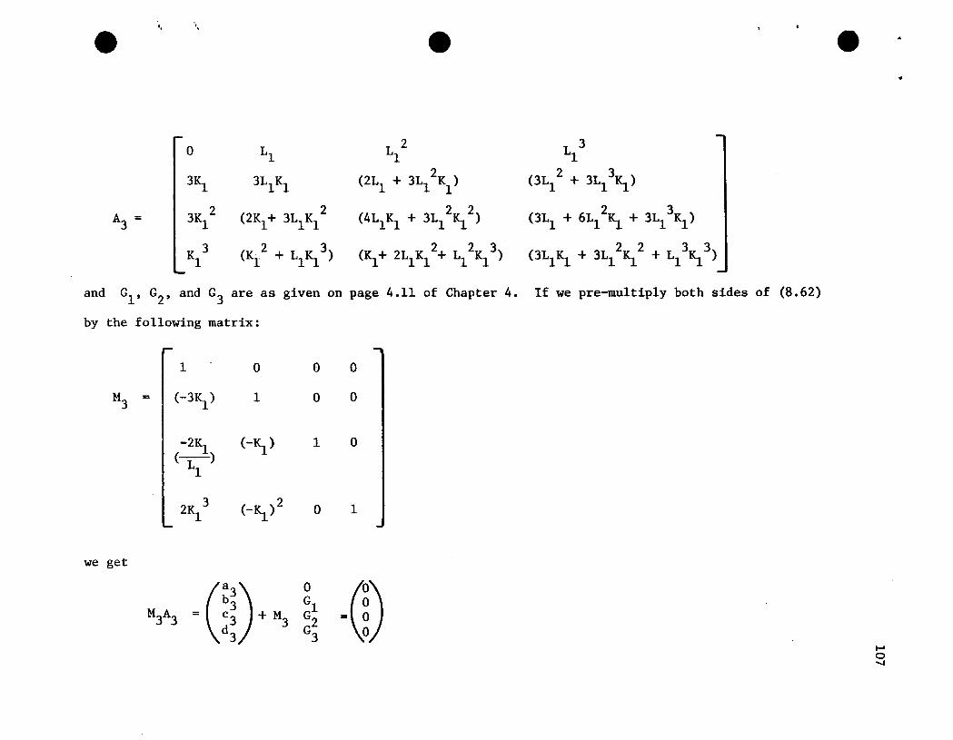
e, ... " e e ~

•

0 L1L 2 L 3

1 1

3K1 3L1K1 (2L1 + 3L12K

1) 2 3(3L1 + 3L1 K1)

I 3K12 2 2 2 2 3A = (2K1+ 3L1K1 (4L1K1 + 3L1 K1 ) (3L1 + 6L1 ~ + 3L1 K1)3

K 3 2 3 2 2 3 2 2 3 31 (Kr + L1~ ) (K1+ 2L1K1 + L1 K1 ) (3L1K1 + 3L1 K1 + L1 ~ )

and G1 , G2

, and G3 are as given on page 4.11 of Chapter 4. If we pre-mu1tip1y both sides of (8.62)

by the following matrix:

1 0 0 0

M3 = I (-3~) 1 0 0

-2K (-K ) 1 0(_1) 1

L1

2K 3 (-K )2 0 11 1

we get

M3A3 = (~~) +M3 ~~ J~)d3 G3 \~

....o"

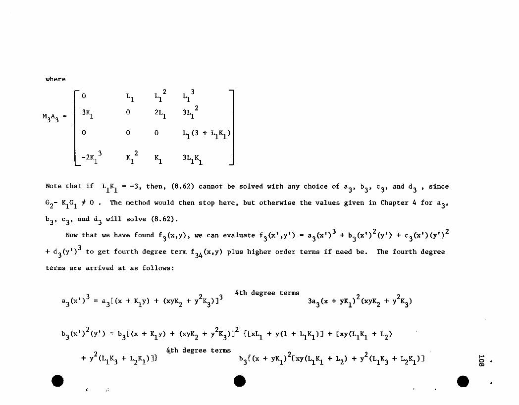
where

0 LIL 2 L 3

I I

M3A3 = I 3!S.0 2LI

3L 2I

0 0 0 LI (3 + LIKI )

-2K 3 K 2 KI 3LI KII I

Note that if LIKI = -3, then, (8.62) cannot be solved with any choice of a3

, b3 , c3, and d3 ' since

G2- KIGI ~ O. The method would then stop here, but otherwise the values given in Chapter 4 for a3,

b3, c3 , and d3 will solve (8.62).

322Now that we have found f 3(x,y), we can evaluate f 3(x',y') = a3(x') + b3

(x') (y') + c3(x')(y')

3+ d3(y') to get fourth degree term f 34 (x,y) plus higher order terms if need be. The fourth degree

terms are arrived at as follows:

a3

(x,)3 = 2 3a3[(x + Kly) + (xyK2 + y K3)]4th degree terms 2 23a3 (x + yKI ) (xyK2 + y K3)

2 2 2b3 (x') (y') = b3[(x + !S.y) + (xyK2 + y K3)] {[xLI + y(l + LIKI )] + [xy(LIKI + L2)

2 (..th degree terms 2 2+ Y (LIK3 + L2KI )]} b3{(x + YR1) [xy(LI!S. + L2) + y (LI K3 + L2RJ)]

el II· - e

.....o •00

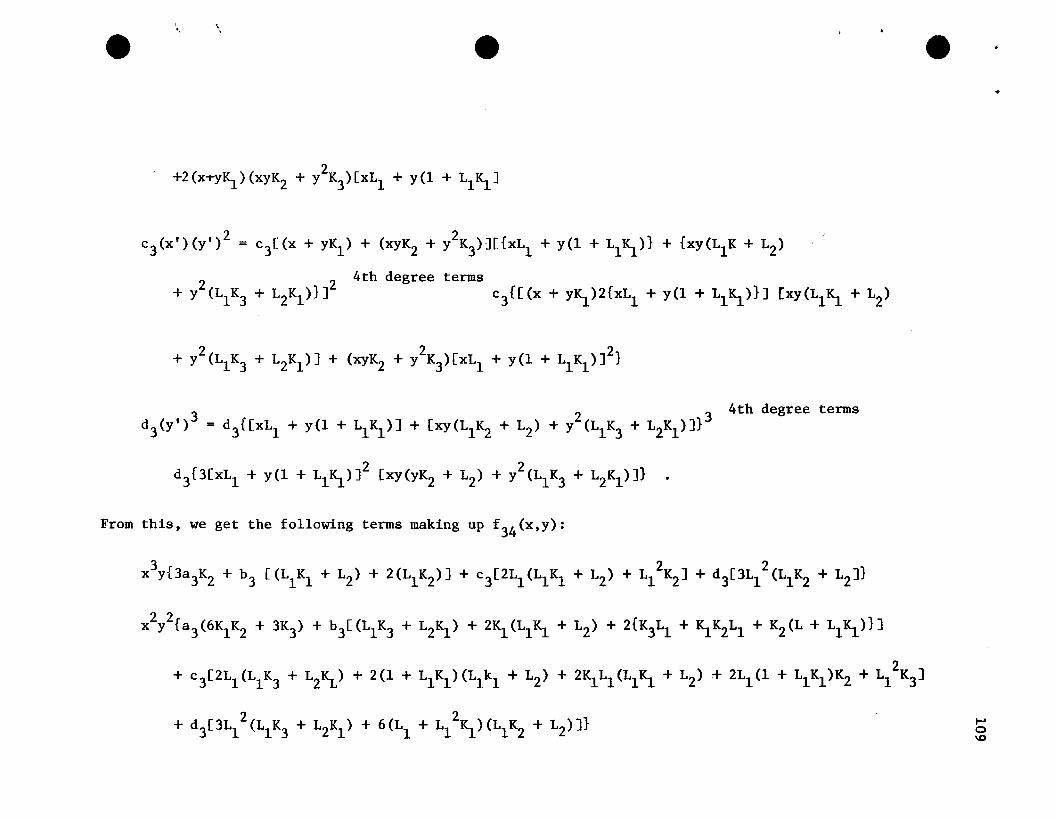
e I,. '.

e

2+2(x~yKl)(xYK2 + Y K3)[xLl + y(l + L1Kl ]

2 2c3(x')(y') = c3[(x + yKl ) + (xyK2 + Y K3)][{xLl + y(l + L1Kl )} + {xy(L1K + L2)

e

2 2+ Y (L1K3 + L2Kl )}]4th degree terms

c3{[(x + y!S.)2{xLl + y(l + L1K1)}] [xy(L1K1 + L2)

2 2 2+ Y (L1K3 + L2Kl )] + (xyK2 + Y K3)[xLl + y(l + L1Kl )] }

d3(y,)3 = d3

{[xLl

+ y(l + L1Kl)] + [xy(L

1K

2+ L2) + y2(L

1K

3+ L

2K

1)]}3

2 2d3{3[xLl + y(l + L1K1)] [xy(yK2 + L2) + y (L1K3 + L2K1)]}

From this, we get the following terms making up f 34 (x,y):

4th degree terms

3 2 2x y{3a3K2 + b3 [(L1Kl + L2) + 2(L1K2)] + c3[2Ll

(L1K1 + L2) + L1 K2] + d3[3L1 (L1K2 + L2]}

22·x y {a3(6K1K2 + 3K3) + b3[(L1K3 + L2~) + 2Kl (L1K1 + L2) + 2{K3L1 + K1K2L1 + K2(L + Ll~)}]

2+ c3[2L1 (L1K3 + L2~) + 2(1 + L1Kl)(Llkl + L2) + 2K1L1 (Ll !S. + L2) + 2Ll (1 + Ll~)K2 + L1 K3]

2 2+ d3[3Ll (L1

K3

+ L2Kl ) + 6(Ll

+ L1 K1)(L1K2 + L2)]} ....o\0

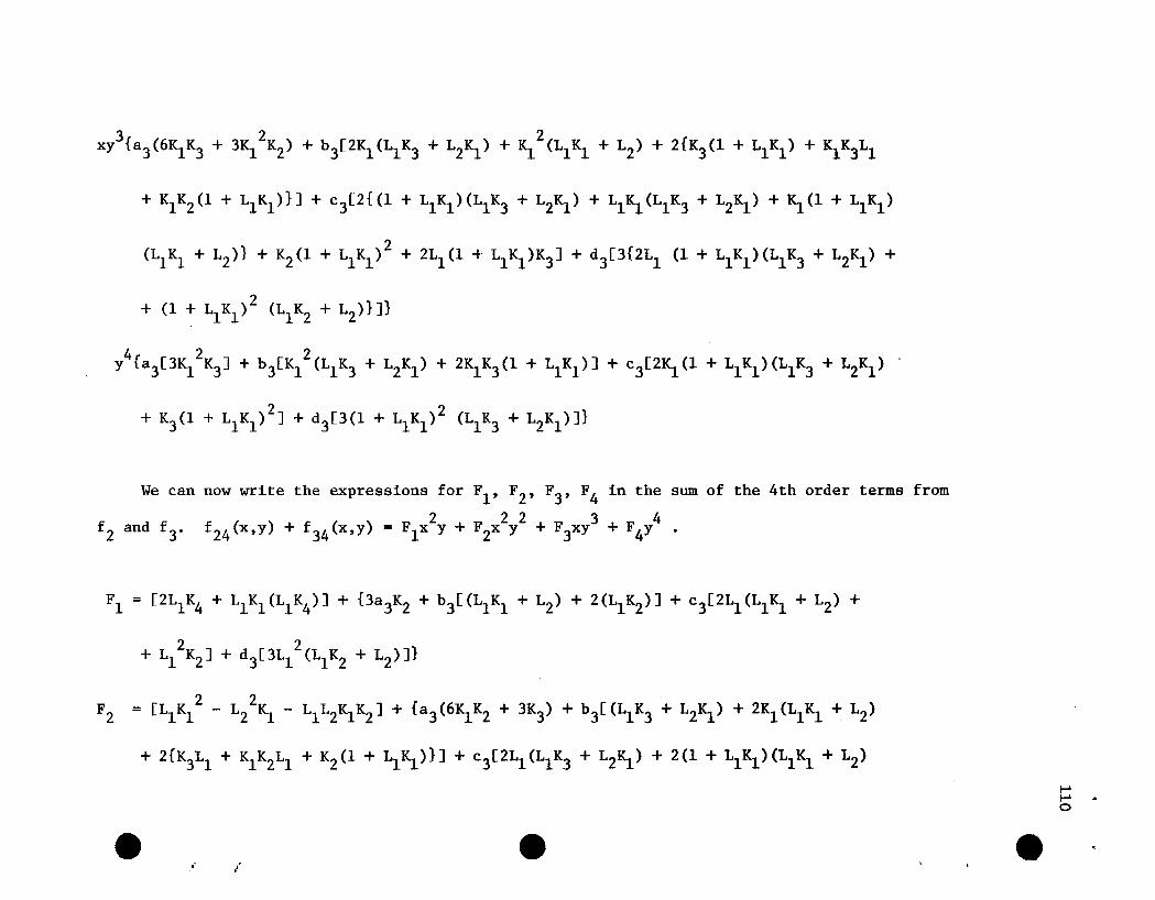
3 Z Zxy {a3(6K1K3 + 3K1 K2) + b3[ZK1 (L1K3 + LZ~) + K1 (L1K1 + LZ) + Z{K3(1 + L1K1) + K1K3L1

+ K1KZ(1 + L1K1)}] + c3[Z{(1 + L1K1) (L1K3 + LZK1) + L1K1 (L1K3 + LZK1) + K1(1 + L1K1)

Z(L1K1 + LZ)} + KZ(l + L1K1) + ZL1(1~· L1K1)K3] + d3[3{ZL1 (1 + L1K1) (L1K3 + LZK1) +

Z+ (1 + L1K1) (L1KZ + LZ)}]}

4 Z Zy {a3[3K1 K3] + b3[K1 (L1K3 + LZK1) + ZK1K3(1 + L1K1)] + c3[ZK1 (1 + L1K1) (L1K3 + L2K1)

2 Z }+ K3(1 + L1K1) ] + d3[3(1 + L1K1) (L1K3 + L2K1)]

We can now write the expressions for F1, F2, F3, F4 in the sum of the 4th order terms from

Z Z Z 3 4f Z and f 3. f Z4 (x,y) + f 34 (x,y) = FIx y + FZx Y + F3xy + F4y

F1 = [ZL1K4 + L1K1 (L1K4)] + {3a3KZ + b3[(L1K1 + LZ) + 2(L1KZ)] + c3[ZLl(Ll~ + LZ) +

Z Z+ L1 KZ] + d3[3L1 (L1KZ + LZ)]}

z ZFZ = [L1K1 - LZ K1 - L1LZK1KZ] + {a3(6K1KZ + 3K3) + b3[(L1K3 + LZ~) + ZK1(L1K1 + LZ)

+ Z{K3L1 + K1KZL1 + KZ(l + L1K1)}] + c3[ZL1(L1K3 + LZ~) + Z(l + Ll~)(LlKl + LZ}

el /

e tit

........ .o

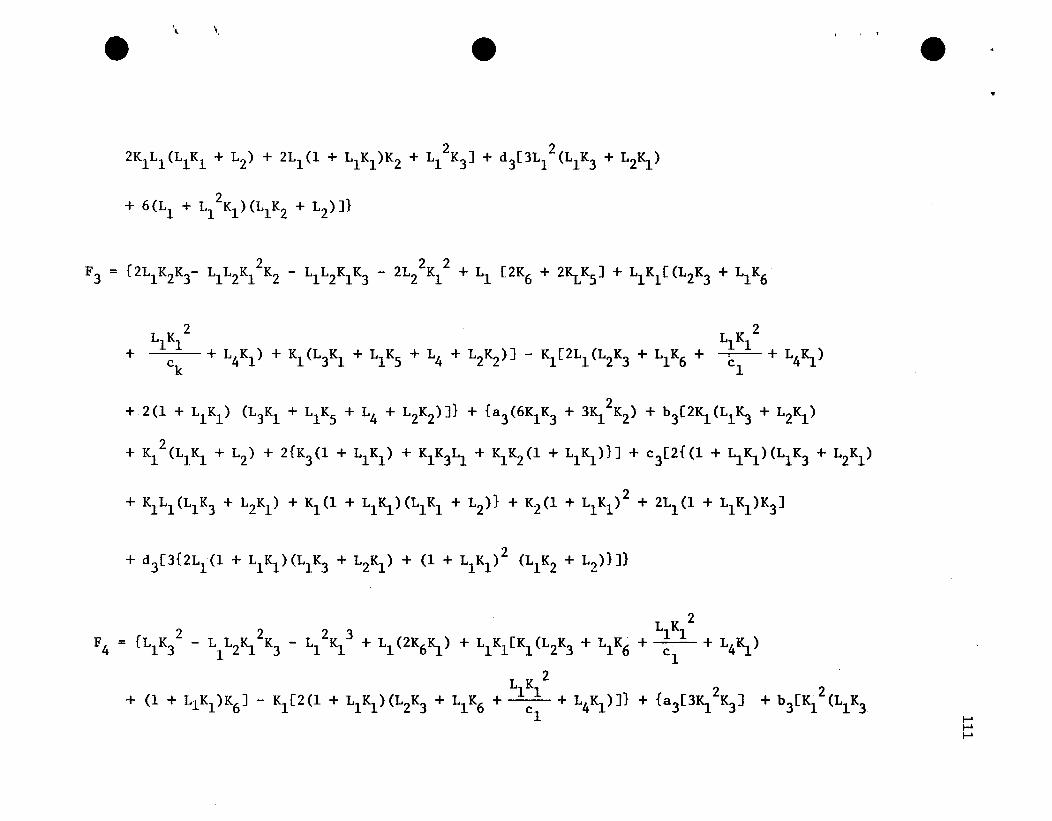
e\ \ e e

Z ZZK1L1(L1K1 + LZ) + ZL1(1 + L1K1)KZ + L1 K3] + d3[3L1 (L1K3 + LZ~)

Z+ 6(L1 + L1 K1)(L1KZ + LZ)]}

Z Z ZF3 = {ZL1KZK3- L1LZK1 KZ - L1LZK1K3 - ZLZ K1 + L1 [ZK6 + 2~K5] + L1K1[(L2K3 + L1K6

L K Z+ --.!.-.!.

ck

ZL1K1

+ L4K1) + K1(L3K1 + L1KS + L4 + LZKZ)] - K1[2L1(LZK3 + L1K6 + c. + L4~)

F =4

z+ Z(l + L1K1) (L3K1 + L1KS + L4 + LZKZ)]} + {a3(6K1K3 + 3K1 KZ) + b3[ZK1(L1K3 + LZK1)

Z+ K1 (L1K1 + LZ) + Z{K3(1 + L1K1) + K1K3L1 + K1KZ(1 + L1K1)}] + c3[Z{(1 + L1K1) (L1K3 + L2K1)

2+ K1L1 (L1K3 + LZK1) + K1(1 + L1K1) (L1K1 + LZ)} + K2(1 + L1~) + 2L1 (1 + L1K1)K3]

+ d3[3{2L1 (1 + L1K1) (L1K3 + LZK1) + (1 + L1K1)Z (L1KZ + L2)}]}

2Z 2 Z 3 .. L1K1

{L1K3 - L1LZK1 K3 - L1 K1 + L1(2K6~) + L1K1[K1(L2K3 + L1K6 + c. + L4~)

ZL1K1 22

+ (1 + L1K1)K6] - K1[2(1 + L1K1) (L2K3 + L1K6 + c. + L4K1)]} + {a3[3~ K3] + b3[~ (L1K3 ...............

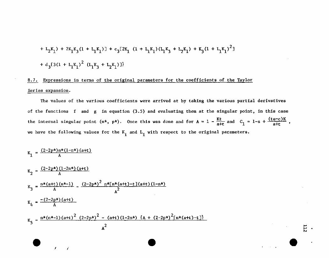
Z+ LZK1) + Z1).K3 (l + Ll 1).)] + c3[Z1). (1 + L1Kl )(L1K3 + LZ1).) + K3 (1 + Ll~) ]

+ d3[3(1 + L1Kl)Z (L1K3 + LZK1)]}

8.7. Expressions in terms of the original parameters for the coefficients of the Taylor

Series expansion.

The values of the various coefficients were arrived at by taking the various partial derivatives

of the functions f and g in equation (3.5) and evaluating them at the singular point, in this case

the internal singular point (n*, p*). Kt (ts-c)KOnce this was done and for A = 1 - a+t and C1 = 1-s + a+t

we have the following values for the Ki and Li with respect to the original parameters.

(Z-Zp*)n*(l-n*) (a+t)1).= .

_ (Z-Zp*)(l-Zn*)(a+t)KZ - A

K = n*(a+t) (n*-l)3 A

K4

= -(Z-zi*)(a+t)

K - n*(n*-l) (a+t)Z5

el i

(Z-Zp*)Z n*[n*(a+t)-t] (a+t) (l-n*)

AZ

Z Z(2-2p*) - (a+t)(l-Zn*) {A + (2-Zp*) [n*(a+t)-t]}

AZ

e e.......... &

N

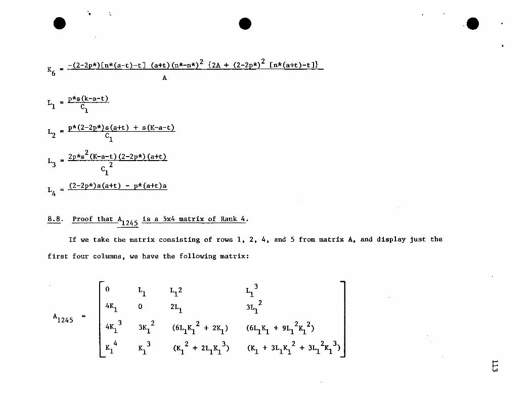
e\• e ·e

K = -(2-2p*)[n*(a-t)-t] (a+t)(n*-n*)2 {2A + (2-2p*)2 [n*(a+t)-t]}6 A

L = p*s(k-a-t)1 C1

_ p*(2-2p*)s(a+t) + s(K-a-t)L2 - C

1

2_ 2p*s (K-a-t)(2-2p*)(a+t)L3 - 2

C1

L = (2-2p*)s(a+t) - p*(a+t)s4

8.8. Proof that A1245 is a 5x4 matrix of Rank 4.

If we take the matrix consisting of rows 1, 2, 4, and 5 from matrix A, and display just the

first four columns, we have the following matrix:

0 Ll Ll 2 L 31

4Kl 0 2L13L 2

1A1245

= I4K 3 3K 2 2 (6Ll~ + 9L12~2)1 1 (6L1Kl + 2K1)

K 4 K 3 2 3 2 2 31 1 (Kl + 2L1K1 ) (Kl + 3Ll Kl + 3L1 Kl )

~

..........w

•

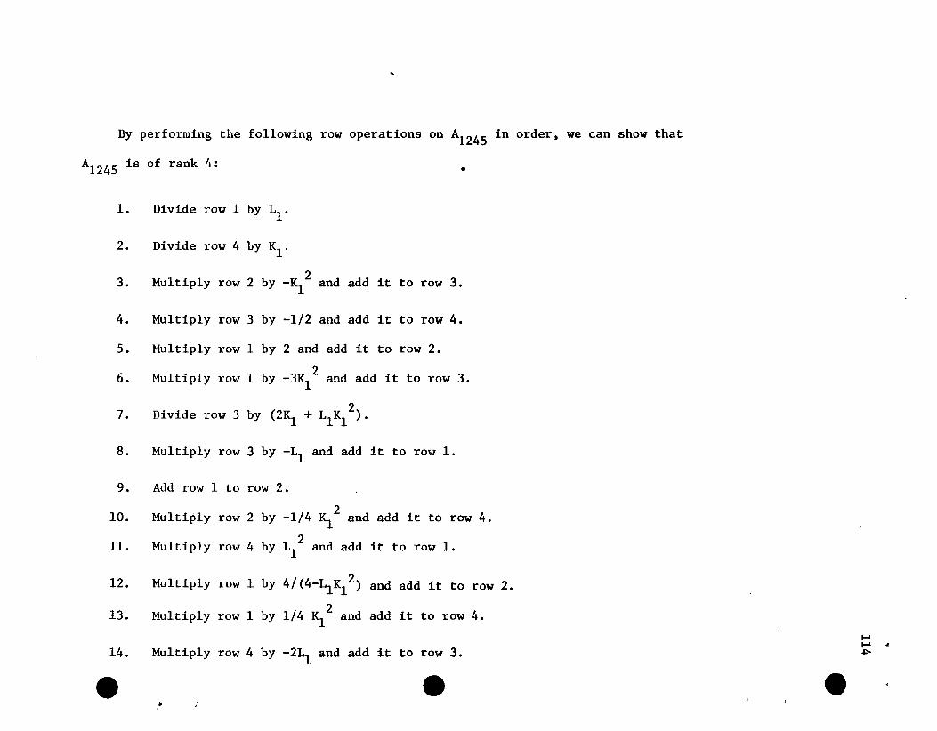
By performing the following row operations on A1245 in order, we can show that

A1245 is of rank 4:

1. Divide row 1 by Ll •

2.

3.

4.

5.

6.

7.

8.

9.

10.

11.

12.

13.

14.

e

Divide row 4 by Kl .

Multiply row 2 by -K1

2 and add it to row 3.

Multiply row 3 by -1/2 and add it to row 4.

Multiply row 1 by 2 and add it to row 2.

Multiply row 1 by -3K12 and add it to row 3.

Divide row 3 by (2~ + Ll K12).

Multiply row 3 by -Ll and add it to row 1.

Add row 1 to row 2.

2Multiply row 2 by -1/4 Kl and add it to row 4.

Multiply row 4 by L12 and add it to row 1.

Multiply row 1 by 4/(4-Ll K12) and add it to row 2.

Multiply row 1 by 1/4 K12 and add it to row 4.

Multiply row 4 by -2Ll and add it to row 3.

e. 'I '

e.......... ..J:'-

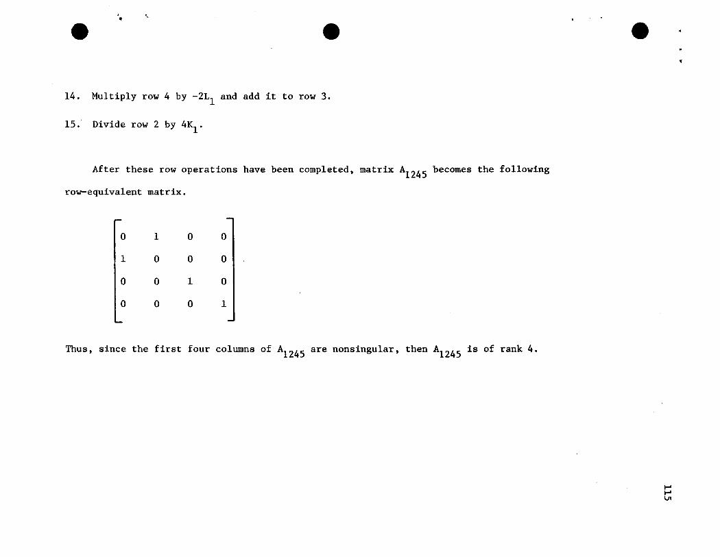
e,. "

e e'I

14. Multiply row 4 by -2Ll and add it to row 3.

15. Divide row 2 by 4Kl

•

After these row operations have been completed, matrix A1245 becomes the following

row-equivalent matrix.

o

1

o

o

1

o

o

o

o

o

1

o

o

o

o

1

Thus, since the first four columns of A1245 are nonsingular, then A1245 is of rank 4.

I-'I-'VI

~ .116

9. LITERATURE CITED

Barrett, J. A. 1978. A model of epidemic development in varietymixtures, in Plant Disease Epidemiology, ed. P. R. Scott andA. Bainbridge. Pages 129-137. Blackwell Scientific Publications,Oxford. 329 pp.

Barrett, J. A. and M. S. Wolfe. 1978. Mu1ti1ines and super-races -­a reply. Phytopathology 68:1537.

Bor1aug, N. E. 1953. New approach to the breeding of wheat varietiesresistant to Puccinia graminis tritici. Phytopathology 43:467.(Abstract).

Browning, J. A. and K. J. Frey. 1969. Multiline cu1tivars as a meansof disease control. Ann. Rev. Phytopathology 7:355-82.

Christianson, F. B. 1975. Hard and soft selection in a subdividedpopulation. Amer. Natur. 109:11-16.

Coddington, E. A. and N. Levinson. 1955. Theory of Ordinary DifferentialEquations. McGraw-Hill, New York. 429 pp.

Crill, P. 1977. An assessment of stabilizing selection in cropvariety development. Ann. Rev. Phytopathology 15:185-202.

Crow, J. F. and M. Kimura. 1970. An Introduction to Population Genetics _Theory. Harper and Row, New York. -

Dempster, E. R. 1955. Maintenance of genetic heterogeneity. ColdSpring Harbor Symposium Quantitative Biology 20:25-32.

Denward, T. 1967. Differentiation in Phytophthora infestans. I. Acomparative study of eight different biotypes. Hereditas 58:191-200.

Fleming, R. A. 1980. Selection pressures and plant pathogens: robust­ness of the model. Phytopathology 70:175-178.

G1iddon, C. and C. Strebeck. 1975. Necessary and sufficient conditionsfor multiple-niche polymorphism in haploids. Amer. Natur. 109:233­235.

Groth, J. V. 1976. Mu1ti1ines and "super-races": a simple model.Phytopathology 66:937-39.

Groth, J. V. and C. O. Person.and parasite in epidemics.

1977. Genetic interdependence of hostAnn. N. Y. Acad. Sci. 287:97-106.

.~

Jayakar, S. C. 1970. A mathematical model for interaction of genefrequencies in a parasite and its host. Theor. Pop. Bio1. 1:140­64.

_ t.

Jensen, N. F.Agron. J.

117

1952. Intra-varietal diversification in oat breeding.44:30-34.

..

Kiyosawa, S. 1972. Theoretical comparison between mixture androtation cultivations of disease resistant varieties. Ann.Phytopathol. Soc. Japan 38:52-59.

Kiyosawa, S. and S. Yabuki. 1976. Modeling on the race frequencychange in a host-pathogen system with genes for resistance andavirulence. Japan J. Breed. 26:237-46.

Kiyosawa, S. and S. Yabuki. 1976. Simulation of race frequencychange in a host-pathogen system with true resistance andavirulence genes. Japan J. Breed. 26:247-55.

laSalle, J. P. 1978. Stability of dynamical systems. Conf~rence

Board of the Mathematical Sciences Regional Conference inMathematics, Mississippi State University, August, 1976. SIAM.

Leonard, K. J. 1969. Selection in heterogeneous populations ofPuccinia graminis f. sp. avenae. Phytopathology 59:1851-57.

Leonard, K. J. 1977. Selection pressures and plant pathogens.Ann. N. Y. Acad. Sci. 287:207-22.

Leonard, K. J. and R. J. Czochor. 1978. In response to 'Selectionpressures and plant pathogens: stability of equilibria'.Phytopathology 68:971-73.

Leonard, K. j. and Czochor, R. J. 1980. Theory of genetic inter­actions among populations of plants and their pathogens. Ann.Rev. Phytopathology 18:237-258.

Levene, H. 1953. Genetic equilibrium when more than one ecologicalniche is available. Amer. Natur. 87:331-333.

Marshall, D. R. andA. J. Prior. 1978. Multiline varieties and diseasecontrol. 1. The "dirty crop" approach with each component carryinga unique single resistance gene. Theor. Appl. Genet. 51:177-84.

Marshall, D. R. and A. J. Prior. 1979. Multiline varieties anddisease control. II. The "dirty crop" approach with componentscarrying two or more genes for resistance. Euphytica 28:145-59.

Marshall, D. R. and B. S. Weir. 1982. Multiline varieties and diseasecontrol. The "dirty crop" approach with complex mixtures ofgenotypes. (in preparation) .

May, R. M. 1973. Stability and Complexity in Model Ecosystems.Princeton University Press. Princeton, New Jersey.

May, R. M. 1974.generations:186:647-647.

Biological populations with nonover1appingstable points, stable cycles, and chaos. Science

•• •118

Mode, C. J. 1958. A mathematical model for the co-evolution ofobligate parasites and their hosts. Evolution 12:158-165.

Mode, C. J. 1960. A model of a host-pathogen system with particularreference to the rusts of cereals. In Biometrical Genetics,ed., Kempthorne, 0., International Union Biological Sciences, Proc.,Series B., No. 38, pp. 84-97.

Mode, C. J. 1961. A generalized model of a host-pathogen system.Biometrics. 17:386-404.

Nelson, R. R. 1972. Stabilizing racial populations of plant pathogensby use of resistance genes. J. Environ. Quality 1:220-27.

Nelson, R. R. 1973. Breeding Plants for Disease Resistance.Pennsylvania State University Press, University Park, Penn.

Nelson, R. R.disease.

1978. Genetics of horizontal resistance to plantAnn. Rev.Phytopathol. 16:359-78.

Nelson, R. R. 1979. The evolution of parasitic fitness. In PlantDisease, Volume IV. How Pathogens Induce Disease., ed. J. G.Horsfall, E. B. Cowling, Academic Press, New York., pages 23-45.

Parlevliet, J. E. and J. C. Zadoks. 1977. The integrated concept ofdisease resistance: a new view including horizontal and verticalresistance in plants. Euphytica 26:5-21. ~

Person, C., J. V. Groth, and O. M. Mylyk. 1976. Genetic change inhost-parasite populations. Ann. Rev. Phytopathol. 14:177-88.

Poincare, J. H. 1885. Sur les courbes definies par les equationsdifferentialles. J. de Mathematiques pures et alliquees. 4neSerie, Tome premier. Pages 167-196.

Robinson, R. A. 1976. Plant Pathosystems. Springer-Verlag, NewYork.

Roughgarden, J. 1979. Theory of Population Genetics and EvolutionaryEcology: An Introduction. Macmillan Publishing Co., Inc., NewYork.

Sedcole, J. R. 1978. Selection pressures and plant pathogens:stability of equilibria. Phytopathology 68:967-70.

Strobeck, C. 1979. Haploid selection with n alleles in m niches.Amer. Natur. 113:439-444.

...

Trenbath, B. R.parasites.

1979. Interactions among diverse hosts and diverseAnn. N. Y. Acad. Sci. 287 124.150.

.... ,.

•'

..a,

• van der Plank, J. E. 1963. Plant Diseases: Epidemics and Control •Academic Press, New York.

van der Plank, J. E. 1968. Disease Resistance in Plants. AcademicPress, New York.

van der Plank, J. E. 1975. Principles of Plant Infection. AcademicPress, New York.

van der Plank, J. E. 1978. Genetic and Molecular Basis of PlantPathogenesis. Springer-Verlag, New York.

van der Vaart, H. R. 1973. A comparative investigation of certaindifference equations and related differential equations:implications for model-building. Bulletin of MathematicalBiology 35:195-211 •

119