-A Starting Point for Analyzing Basketball Statistics.pdf

Journal of Quantitative Analysis inSports

Volume 3, Issue 3 2007 Article 1

A Starting Point for Analyzing BasketballStatistics

Justin Kubatko∗ Dean Oliver†

Kevin Pelton‡ Dan T. Rosenbaum∗∗

∗The Ohio State University and basketball-reference.com, [email protected]†Basketball on Paper and Denver Nuggets, [email protected]‡Seattle Sonics & Storm, [email protected]∗∗University of North Carolina at Greensboro and Cleveland Cavaliers,

[email protected]

Copyright c©2007 The Berkeley Electronic Press. All rights reserved.

A Starting Point for Analyzing BasketballStatistics∗

Justin Kubatko, Dean Oliver, Kevin Pelton, and Dan T. Rosenbaum

Abstract

The quantitative analysis of sports is a growing branch of science and, in many ways onethat has developed through non-academic and non-traditionally peer-reviewed work. The aim ofthis paper is to bring to a peer-reviewed journal the generally accepted basics of the analysis ofbasketball, thereby providing a common starting point for future research in basketball. The pos-session concept, in particular the concept of equal possessions for opponents in a game, is centralto basketball analysis. Estimates of possessions have existed for approximately two decades, butthe various formulas have sometimes created confusion. We hope that by showing how most pre-vious formulas are special cases of our more general formulation, we shed light on the relationshipbetween possessions and various statistics. Also, we hope that our new estimates can provide acommon basis for future possession estimation. In addition to listing data sources for statisticalresearch on basketball, we also discuss other concepts and methods, including offensive and de-fensive ratings, plays, per-minute statistics, pace adjustments, true shooting percentage, effectivefield goal percentage, rebound rates, Four Factors, plus/minus statistics, counterpart statistics, lin-ear weights metrics, individual possession usage, individual efficiency, Pythagorean method, andBell Curve method. This list is not an exhaustive list of methodologies used in the field, but webelieve that they provide a set of tools that fit within the possession framework and form the basisof common conversations on statistical research in basketball.

KEYWORDS: basketball possessions, offensive ratings, defensive ratings, plays, per-minutestatistics, pace adjustments, true shooting percentage, effective field goal percentage, reboundrates, Four Factors, plus/minus statistics, counterpart statistics, linear weights metrics, individualpossession usage, individual efficiency, Pythagorean method, Bell Curve method

∗We would like to thank two anonymous referees, Javier Gonzalez, Thomas Ryan, Steven Schran,and the APBRmetrics community for years of commentary and critique of the ideas contained inthis paper. We also would like to make it clear that this paper represents the views of the authorsalone and not the organizations that the authors are associated with.

1. Introduction

One of the great strengths of the quantitative analysis of sports is that it is a melting pot for ideas. It blends together ideas from several academic disciplines with ideas of hobbyists and practitioners from outside academia. It is a true “marketplace of ideas” and one where good ideas often are implemented immediately into practice. But this plethora of voices can lead to disparities in the basic concepts and terminology that different groups use to express their ideas. That can create barriers when one group tries to communicate its ideas to another group. It also raises the costs to new entrants into the field. In addition, it makes it harder for the large number of interested readers with varied backgrounds to evaluate the arguments and evidence. In this article, we define the basic variables used in what is now the mainstream of basketball statistics. Originating primarily from non-academic sources, in particular Oliver (2004) and Hollinger (2003, 2004, and 2005), this body of work has withstood review from peers practicing in the NBA, writers, some academics, and a variety of critics interested in the material purely for its entertainment value. While this framework for evaluating basketball has been built largely outside of academic circles, it has been influenced by the large number of academic articles on basketball research published in journals on management, sociology, statistics, psychology, medicine, and economics. We hope that introduction of this work into the Journal of Quantitative Analysis of Sports will provide a peer-reviewed foundation from which academic basketball researchers can launch their research. By outlining the framework here, we anticipate that the work from academic sources focusing on smaller points of interest can ultimately be cast in terms of that framework. That framework should provide some uniformity of communication for both researchers and lay readers. As we introduce the basic variables of basketball analysis, we use a variety of available data sources to describe the distributions of these variables. Because the concept of “possessions” plays such a central role in analyzing basketball, we undertake an extensive analysis of possessions using four seasons of game log data.1 And finally, we provide a detailed listing of the sources of data for analyzing basketball statistics, which we hope will help jump start more research on basketball.

1 Oliver (2004), Hollinger (2003, 2004, and 2005), and Berri et al. (2006) all use possessions as the foundation for their analyses of basketball statistics.

1

Kubatko et al.: A Starting Point for Analyzing Basketball Statistics

Published by The Berkeley Electronic Press, 2007

2. Defining Possessions: the Starting Point of Basketball Statistics

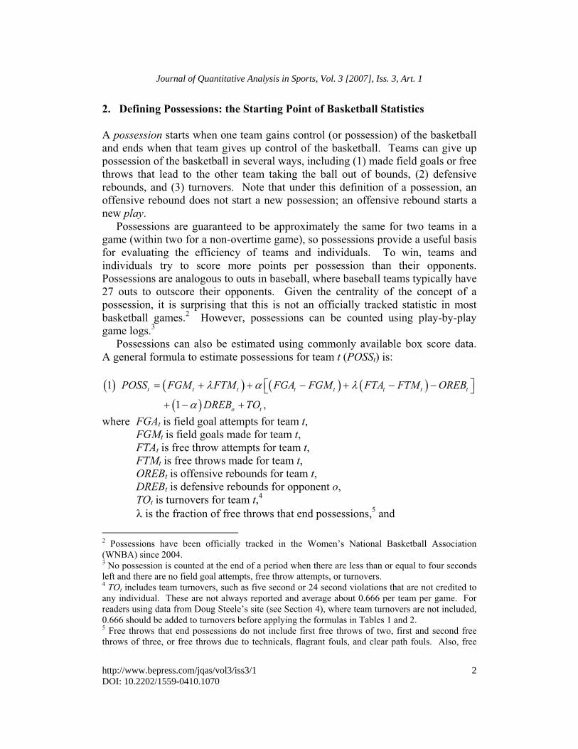
A possession starts when one team gains control (or possession) of the basketball and ends when that team gives up control of the basketball. Teams can give up possession of the basketball in several ways, including (1) made field goals or free throws that lead to the other team taking the ball out of bounds, (2) defensive rebounds, and (3) turnovers. Note that under this definition of a possession, an offensive rebound does not start a new possession; an offensive rebound starts a new play. Possessions are guaranteed to be approximately the same for two teams in a game (within two for a non-overtime game), so possessions provide a useful basis for evaluating the efficiency of teams and individuals. To win, teams and individuals try to score more points per possession than their opponents. Possessions are analogous to outs in baseball, where baseball teams typically have 27 outs to outscore their opponents. Given the centrality of the concept of a possession, it is surprising that this is not an officially tracked statistic in most basketball games.2 However, possessions can be counted using play-by-play game logs.3 Possessions can also be estimated using commonly available box score data. A general formula to estimate possessions for team t (POSSt) is:

� � � � � � � ��

1

1 ,t t t t t t t t

o t

POSS FGM FTM FGA FGM FTA FTM OREB

DREB TO

� � �

�

� ��

where FGAt is field goal attempts for team t,FGMt is field goals made for team t,FTAt is free throw attempts for team t,FTMt is free throws made for team t,OREBt is offensive rebounds for team t,DREBt is defensive rebounds for opponent o,TOt is turnovers for team t,4

� is the fraction of free throws that end possessions,5 and

2 Possessions have been officially tracked in the Women’s National Basketball Association (WNBA) since 2004. 3 No possession is counted at the end of a period when there are less than or equal to four seconds left and there are no field goal attempts, free throw attempts, or turnovers. 4 TOt includes team turnovers, such as five second or 24 second violations that are not credited to any individual. These are not always reported and average about 0.666 per team per game. For readers using data from Doug Steele’s site (see Section 4), where team turnovers are not included, 0.666 should be added to turnovers before applying the formulas in Tables 1 and 2. 5 Free throws that end possessions do not include first free throws of two, first and second free throws of three, or free throws due to technicals, flagrant fouls, and clear path fouls. Also, free

2

Journal of Quantitative Analysis in Sports, Vol. 3 [2007], Iss. 3, Art. 1

http://www.bepress.com/jqas/vol3/iss3/1DOI: 10.2202/1559-0410.1070

� is a parameter between zero and one.

Equation (1) recognizes that each turnover, made field goal, and made possession-ending free throw constitutes a possession, i.e. has a possession value of one. Missed field goal attempts and missed possession-ending free throw attempts share credit for the possession with defensive rebounds. Missed field goal attempts and missed possession-ending free throw attempts get an � share of the possession, while the defensive rebound gets a 1 – � share. Offensive rebounds undo missed field goal attempts and missed possession-ending free throw attempts, so their possession value is -�. One of the most common (and simplest) formulations of (1) is to assume that �= 1 and � = 0.44, which results in the following formula for possessions:

(2) POSSt = FGAt + 0.44 × FTAt – OREBt + TOt.

This formulation sometimes is referred to as possessions lost, but it is important to note that it implies that defensive rebounds have no possession value. Another common formulation, possessions gained, assumes that � = 0 and implies that offensive rebounds, missed field goal attempts, and missed possession-ending free throw attempts have no possession value.6

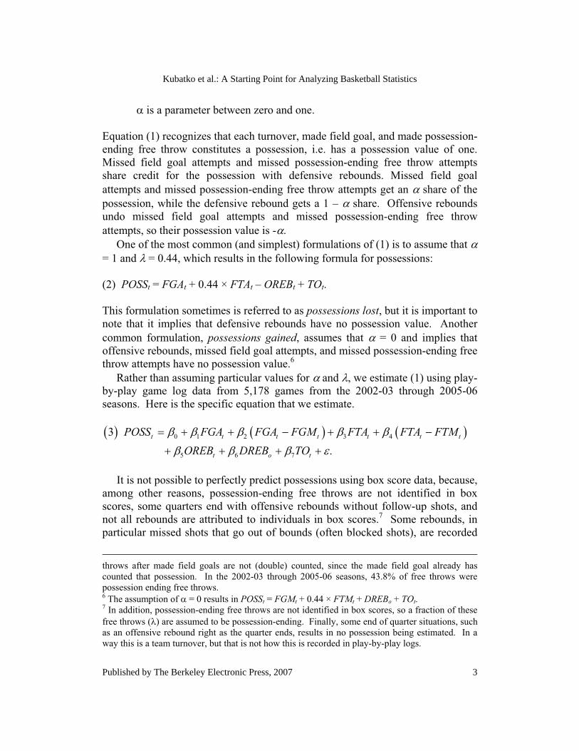
Rather than assuming particular values for � and �, we estimate (1) using play-by-play game log data from 5,178 games from the 2002-03 through 2005-06 seasons. Here is the specific equation that we estimate.

� � � � � �0 1 2 3 4

5 6 7

3.

t t t t t t t

t o t

POSS FGA FGA FGM FTA FTA FTMOREB DREB TO

�

�

It is not possible to perfectly predict possessions using box score data, because, among other reasons, possession-ending free throws are not identified in box scores, some quarters end with offensive rebounds without follow-up shots, and not all rebounds are attributed to individuals in box scores.7 Some rebounds, in particular missed shots that go out of bounds (often blocked shots), are recorded

throws after made field goals are not (double) counted, since the made field goal already has counted that possession. In the 2002-03 through 2005-06 seasons, 43.8% of free throws were possession ending free throws. 6 The assumption of � = 0 results in POSSt = FGMt + 0.44 × FTMt + DREBo + TOt.7 In addition, possession-ending free throws are not identified in box scores, so a fraction of these free throws (�) are assumed to be possession-ending. Finally, some end of quarter situations, such as an offensive rebound right as the quarter ends, results in no possession being estimated. In a way this is a team turnover, but that is not how this is recorded in play-by-play logs.

3



as team rebounds.8 For this reason we estimate (3) without imposing all of the restrictions in (1); this more flexible form allows us to capture relationships between these variables and other factors, such as team rebounds, that we do not include in the model. We estimate (3) for both teams’ possessions in a game averaged together, because we find that the best predictor of a particular team’s number of possessions is the average estimated using both teams rather than the estimated number for just that specific team.9

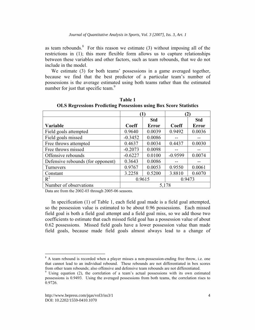
Table 1 OLS Regressions Predicting Possessions using Box Score Statistics

(1) (2)

Variable Coeff Std

Error Coeff Std

ErrorField goals attempted 0.9640 0.0039 0.9492 0.0036 Field goals missed -0.3452 0.0086 -- -- Free throws attempted 0.4637 0.0034 0.4437 0.0030 Free throws missed -0.2073 0.0098 -- -- Offensive rebounds -0.6227 0.0100 -0.9599 0.0074 Defensive rebounds (for opponent) 0.3643 0.0086 -- -- Turnovers 0.9767 0.0053 0.9550 0.0061 Constant 3.2258 0.5200 3.8810 0.6070 R2 0.9615 0.9473 Number of observations 5,178 Data are from the 2002-03 through 2005-06 seasons.

In specification (1) of Table 1, each field goal made is a field goal attempted, so the possession value is estimated to be about 0.96 possessions. Each missed field goal is both a field goal attempt and a field goal miss, so we add those two coefficients to estimate that each missed field goal has a possession value of about 0.62 possessions. Missed field goals have a lower possession value than made field goals, because made field goals almost always lead to a change of

8 A team rebound is recorded when a player misses a non-possession-ending free throw, i.e. one that cannot lead to an individual rebound. These rebounds are not differentiated in box scores from other team rebounds; also offensive and defensive team rebounds are not differentiated. 9 Using equation (2), the correlation of a team’s actual possessions with its own estimated possessions is 0.9493. Using the averaged possessions from both teams, the correlation rises to 0.9726.

4



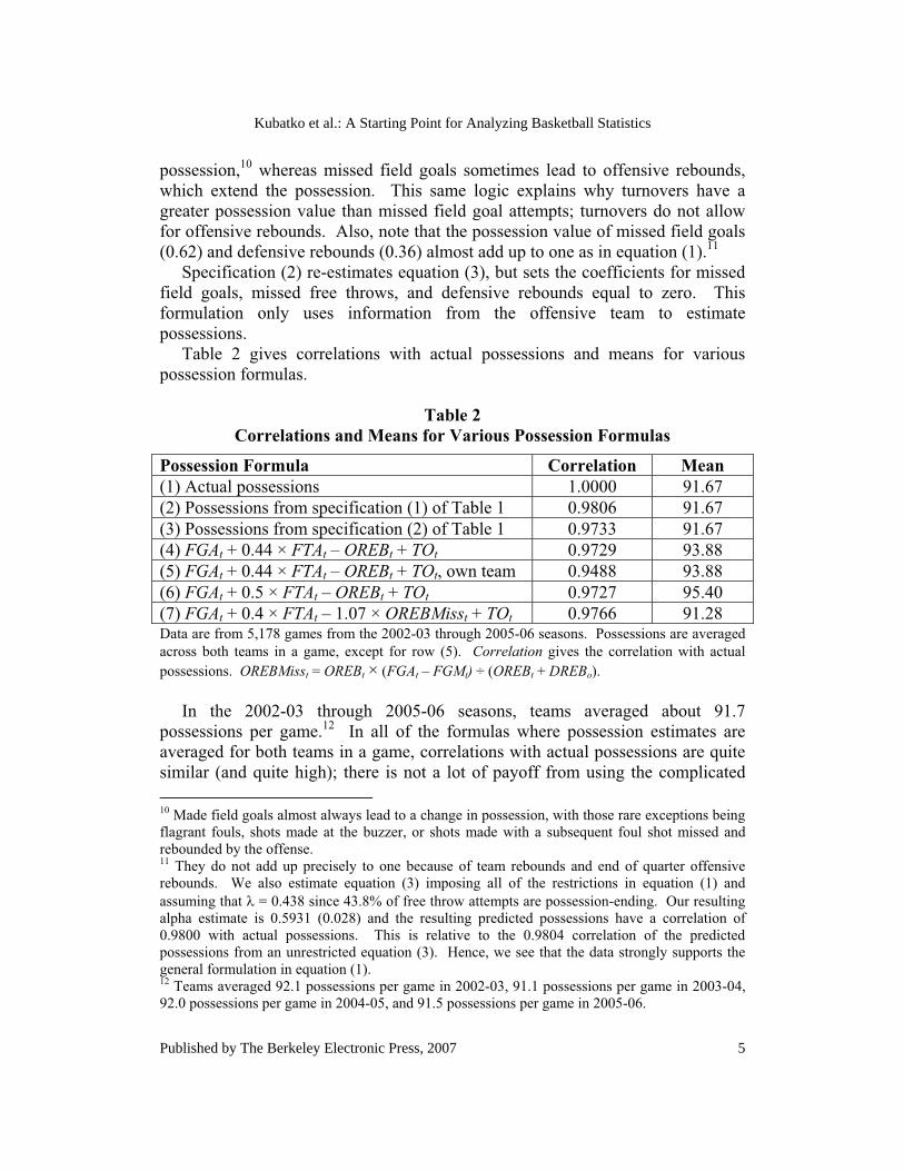
possession,10 whereas missed field goals sometimes lead to offensive rebounds, which extend the possession. This same logic explains why turnovers have a greater possession value than missed field goal attempts; turnovers do not allow for offensive rebounds. Also, note that the possession value of missed field goals (0.62) and defensive rebounds (0.36) almost add up to one as in equation (1).11 Specification (2) re-estimates equation (3), but sets the coefficients for missed field goals, missed free throws, and defensive rebounds equal to zero. This formulation only uses information from the offensive team to estimate possessions. Table 2 gives correlations with actual possessions and means for various possession formulas.

Table 2 Correlations and Means for Various Possession Formulas

Possession Formula Correlation Mean (1) Actual possessions 1.0000 91.67 (2) Possessions from specification (1) of Table 1 0.9806 91.67 (3) Possessions from specification (2) of Table 1 0.9733 91.67 (4) FGAt + 0.44 × FTAt – OREBt + TOt 0.9729 93.88 (5) FGAt + 0.44 × FTAt – OREBt + TOt, own team 0.9488 93.88 (6) FGAt + 0.5 × FTAt – OREBt + TOt 0.9727 95.40 (7) FGAt + 0.4 × FTAt – 1.07 × OREBMisst + TOt 0.9766 91.28 Data are from 5,178 games from the 2002-03 through 2005-06 seasons. Possessions are averaged across both teams in a game, except for row (5). Correlation gives the correlation with actual possessions. OREBMisst = OREBt × (FGAt – FGMt) ÷ (OREBt + DREBo). In the 2002-03 through 2005-06 seasons, teams averaged about 91.7 possessions per game.12 In all of the formulas where possession estimates are averaged for both teams in a game, correlations with actual possessions are quite similar (and quite high); there is not a lot of payoff from using the complicated 10 Made field goals almost always lead to a change in possession, with those rare exceptions being flagrant fouls, shots made at the buzzer, or shots made with a subsequent foul shot missed and rebounded by the offense. 11 They do not add up precisely to one because of team rebounds and end of quarter offensive rebounds. We also estimate equation (3) imposing all of the restrictions in equation (1) and assuming that � = 0.438 since 43.8% of free throw attempts are possession-ending. Our resulting alpha estimate is 0.5931 (0.028) and the resulting predicted possessions have a correlation of 0.9800 with actual possessions. This is relative to the 0.9804 correlation of the predicted possessions from an unrestricted equation (3). Hence, we see that the data strongly supports the general formulation in equation (1). 12 Teams averaged 92.1 possessions per game in 2002-03, 91.1 possessions per game in 2003-04, 92.0 possessions per game in 2004-05, and 91.5 possessions per game in 2005-06.

5



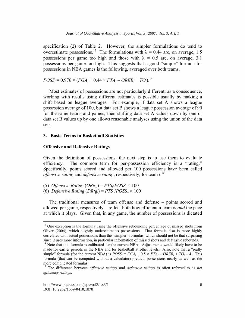
specification (2) of Table 2. However, the simpler formulations do tend to overestimate possessions.13 The formulations with � = 0.44 are, on average, 1.5 possessions per game too high and those with � = 0.5 are, on average, 3.1 possessions per game too high. This suggests that a good “simple” formula for possessions in NBA games is the following, averaged over both teams.

POSSt = 0.976 × (FGAt + 0.44 × FTAt – OREBt + TOt).14

Most estimates of possessions are not particularly different; as a consequence, working with results using different estimates is possible usually by making a shift based on league averages. For example, if data set A shows a league possession average of 100, but data set B shows a league possession average of 99 for the same teams and games, then shifting data set A values down by one or data set B values up by one allows reasonable analyses using the union of the data sets.

3. Basic Terms in Basketball Statistics

Offensive and Defensive Ratings

Given the definition of possessions, the next step is to use them to evaluate efficiency. The common term for per-possession efficiency is a “rating.” Specifically, points scored and allowed per 100 possessions have been called offensive rating and defensive rating, respectively, for team t.15

(5) Offensive Rating (ORtgt) = PTSt/POSSt × 100 (6) Defensive Rating (DRtgt) = PTSo/POSSo × 100

The traditional measures of team offense and defense – points scored and allowed per game, respectively – reflect both how efficient a team is and the pace at which it plays. Given that, in any game, the number of possessions is dictated

13 One exception is the formula using the offensive rebounding percentage of missed shots from Oliver (2004), which slightly underestimates possessions. That formula also is more highly correlated with actual possessions than the “simpler” formulas, which should not be that surprising since it uses more information, in particular information of missed shots and defensive rebounds. 14 Note that this formula is calibrated for the current NBA. Adjustments would likely have to be made for earlier periods in the NBA and for basketball at other levels. Also, note that a “really simple” formula (for the current NBA) is POSSt = FGAt + 0.5 × FTAt – OREBt + TOt – 4. This formula (that can be computed without a calculator) predicts possessions nearly as well as the more complicated formulas. 15 The difference between offensive ratings and defensive ratings is often referred to as netefficiency ratings.

6



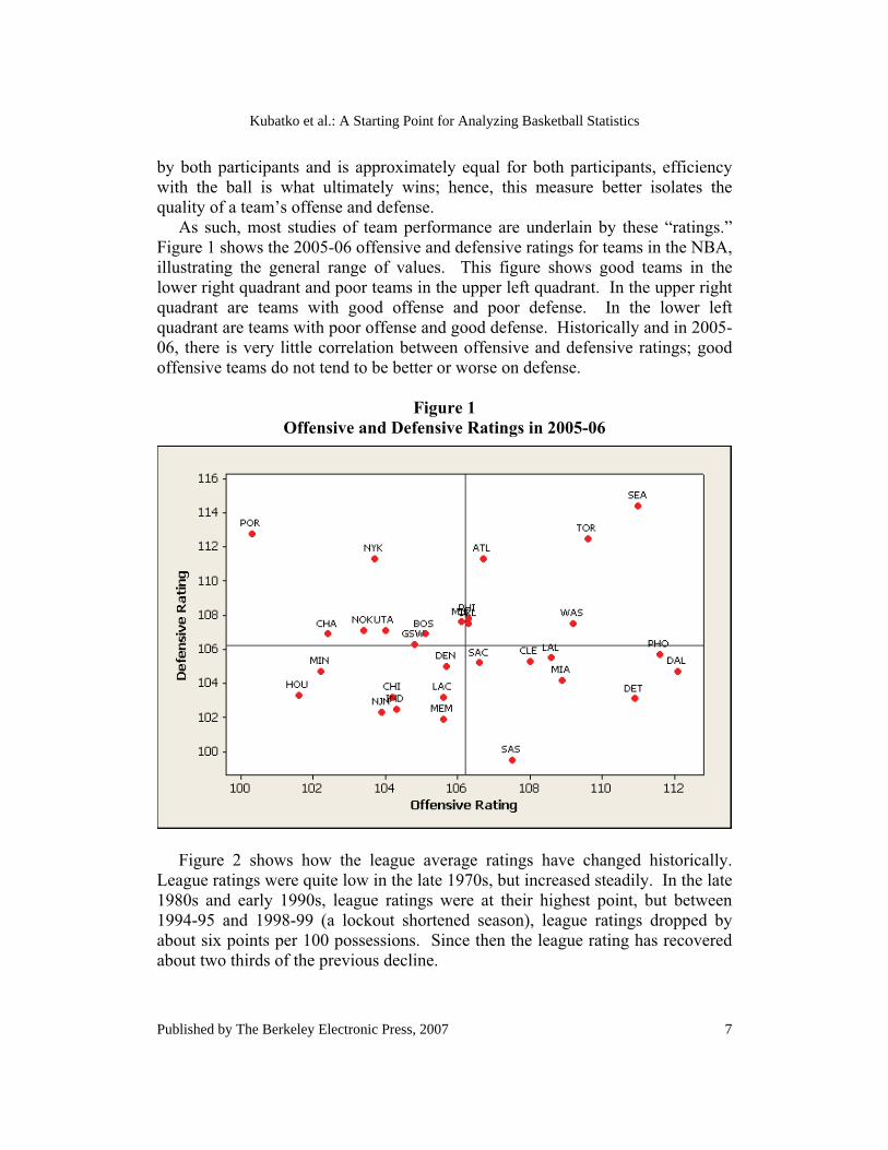
by both participants and is approximately equal for both participants, efficiency with the ball is what ultimately wins; hence, this measure better isolates the quality of a team’s offense and defense. As such, most studies of team performance are underlain by these “ratings.” Figure 1 shows the 2005-06 offensive and defensive ratings for teams in the NBA, illustrating the general range of values. This figure shows good teams in the lower right quadrant and poor teams in the upper left quadrant. In the upper right quadrant are teams with good offense and poor defense. In the lower left quadrant are teams with poor offense and good defense. Historically and in 2005-06, there is very little correlation between offensive and defensive ratings; good offensive teams do not tend to be better or worse on defense.

Figure 1 Offensive and Defensive Ratings in 2005-06

Figure 2 shows how the league average ratings have changed historically. League ratings were quite low in the late 1970s, but increased steadily. In the late 1980s and early 1990s, league ratings were at their highest point, but between 1994-95 and 1998-99 (a lockout shortened season), league ratings dropped by about six points per 100 possessions. Since then the league rating has recovered about two thirds of the previous decline.

7



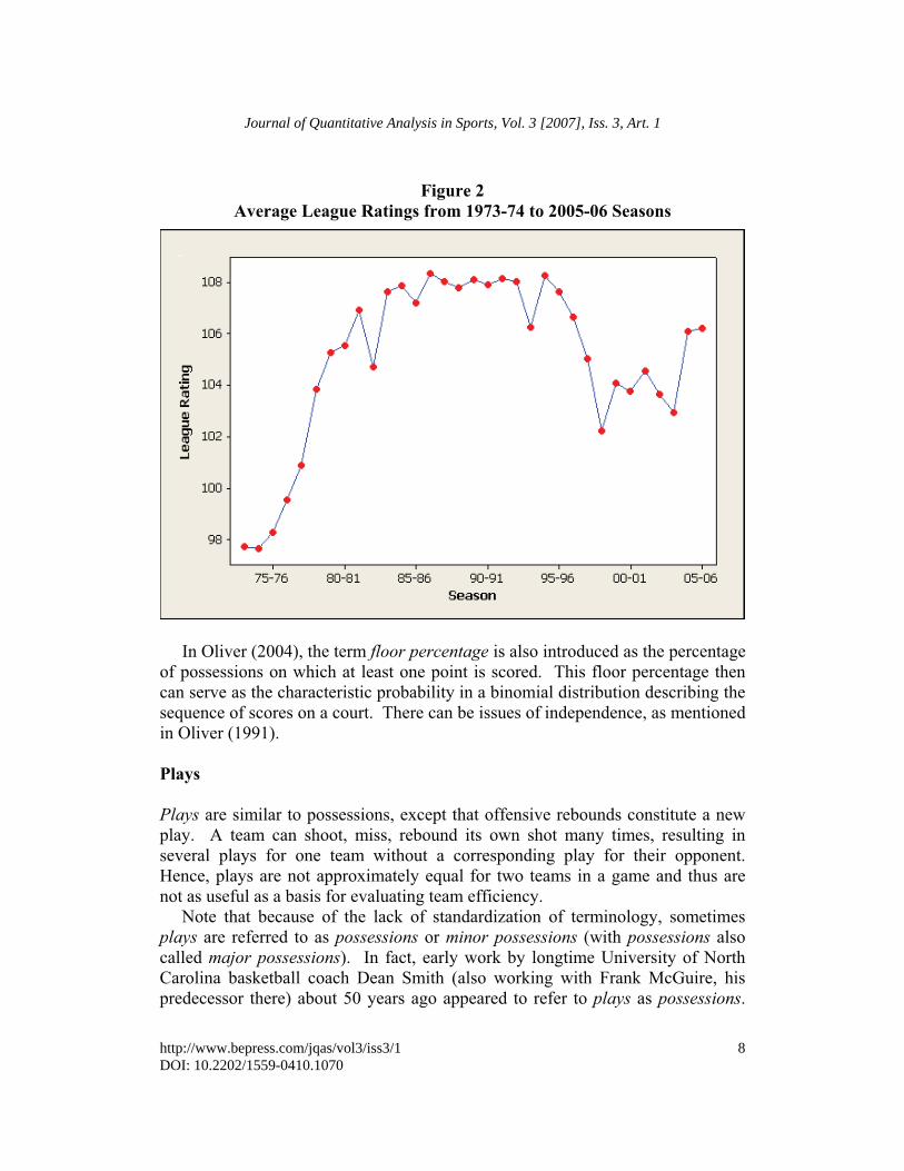
Figure 2 Average League Ratings from 1973-74 to 2005-06 Seasons

In Oliver (2004), the term floor percentage is also introduced as the percentage of possessions on which at least one point is scored. This floor percentage then can serve as the characteristic probability in a binomial distribution describing the sequence of scores on a court. There can be issues of independence, as mentioned in Oliver (1991).

Plays

Plays are similar to possessions, except that offensive rebounds constitute a new play. A team can shoot, miss, rebound its own shot many times, resulting in several plays for one team without a corresponding play for their opponent. Hence, plays are not approximately equal for two teams in a game and thus are not as useful as a basis for evaluating team efficiency. Note that because of the lack of standardization of terminology, sometimes plays are referred to as possessions or minor possessions (with possessions also called major possessions). In fact, early work by longtime University of North Carolina basketball coach Dean Smith (also working with Frank McGuire, his predecessor there) about 50 years ago appeared to refer to plays as possessions.

8



Due to the obvious potential for confusion, the authors do not recommend using the term possessions when speaking about plays. The number of plays can be counted, but it is often estimated as:

(7) PLAYSt = FGAt + 0.44 × FTAt + TOt.

As mentioned above with our study on possessions, the multiplying factor on FTAt is related to the fraction of free throws that are end possessions. On average, in the 2002-03 through 2005-06 seasons, teams had 105.0 plays (both actual and estimated) on their 91.7 possessions. Analogous to floor percentage, the percentage of plays on which at least one point is scored is called the play percentage.

Per-Minute Statistics

Another important breakthrough for analysis of the NBA was finding that statistics calculated on a per-minute basis tend to be fairly consistent even when a player's minutes played are variable. This allows for direct comparisons of starters and reserves who play fewer minutes (per-minute statistics become unreliable for players who have played very few minutes; generally, 500 or 1,000 minutes played in an NBA season is used as a cut-off point). Sometimes, per-minute statistics are referred to as rates; the scoring rate for player p, for example, is points scored per 40 minutes (PTS40p):

(8) PTS40p = PTSp/MINp × 40,

where PTSp is points for player p and MINp is minutes for player p. The use of per-minute statistics allowed analysts to identify young players like Andrei Kirilenko, Michael Redd and Zach Randolph as candidates to break out when they had the opportunity to play more minutes. Hollinger (2003, 2004, 2005) has used a basis of 40 minutes despite NBA games being 48 minutes long. Because college and international games are 40 minutes long and NBA players rarely play more than 40 minutes per game, this basis can have its benefits for consistency across different leagues. For that reason we have a slight preference for using 40 minutes as a basis, although the number of minutes used as a basis does not alter the effectiveness of per-minute statistics. We will use a 40 minute basis for consistency throughout the rest of this article.

9



Pace Adjustments

A team that averages 100 possessions per game gives their team 25 percent more chances to shoot, assist, rebound, etc. than a team that averages 80 possessions per game. Hence, many basketball analysts pace adjust their team and player statistics.

(9) adjPTS40p = PTS40p × (POSSl/POSSt),

where POSSl is the league average for possessions per game.

True Shooting Percentage and Effective Field Goal Percentage

Field goal percentage (FG%) does not account for three pointers or free throws, so two common alternatives have been developed: effective field goal percentage(eFG%) and true shooting percentage (TS%). These can be measured at the individual or team level.

(10) FG% = FGM/FGA.(11) eFG% = (FGM + 0.5 × 3PM)/FGA.(12) TS% = (PTS/2)/(FGA + 0.44 × FTA).16

Effective field goal percentage accounts for made three pointers (3PM), whereas true shooting percentage accounts for both three pointers and free throws. True shooting percentage provides a measure of total efficiency in scoring attempts, while effective field goal percentage isolates a player’s (or team’s) shooting efficiency from the field. Both measures are appropriate for different situations; the authors would not advocate one or the other for exclusive use. Over the 1996-97 through 2005-06 seasons, means (and standard deviations) for the three measures, measured at the player level, are as follows.17

� FG% = 44.6% (4.7%) � eFG% = 47.9% (4.4%) � TS% = 52.3% (4.5%)

16 Points per shot is used at times and is analogous to TS%, with a formula of PTS/(FGA + 0.44 × FTA).17 These shooting percentage measures are weighted by field goal attempts.

10



Rebound Rate

Per-minute rebound statistics are affected not only by the pace at which different teams play, but also their ability to make shots and force opponents to miss. As a result, rebounding is best evaluated by the percentage of all missed shots a player rebounds when they are in the game. (This is usually estimated by their team’s rebounds per minute added to opponent rebounds per minute and multiplied by the player's minutes.) This is known as rebound rate or rebound percentage for player p (REB%p).

(13) % p pp

t o t

REB MINREB

REB REB MIN� � � �

� � � � �� ,

where REBp is rebounds for player p, REBt is rebounds for team t, and REBo is rebounds for the opponents o of team t, MINp is minutes for player p, and MINt is minutes for team t. Player rebounding percentage can also be split into offensive rebounding percentage (OREB%p) and defensive rebounding percentage(DREB%p), which can prove insightful because few players are equally adept at rebounding on both ends of the court.

� �

� �

14 %

15 %

p pp

t o t

p pp

o t t

OREB MINOREB

OREB DREB MIN

DREB MINDREB

OREB DREB MIN

� � � ��

� � � ��

At the team level, rebound percentage is also a more accurate measure of ability than rebounds per game. Good teams tend to grab more rebounds than their opponents because they have fewer missed shots than their opponents, Missed shots tend to be predominantly rebounded by defensive teams. Team rebounding percentage isolates rebounding ability from the ability to force misses. The total team rebounding percentage (REB%t) is the average of its offensive rebounding percentage (OREB%t) and defensive rebounding percentage(DREB%t), which are defined below:

11



� �

� �

� �

16 %

17 %

% %18 %2

tt

t o

tt

o t

t tt

OREBOREBOREB DREB

DREBDREBOREB DREB

OREB DREBREB

�

�

�

At the team level, there is a negative relationship between offensive and defensive rebounding percentages (over the 1996-97 through 2005-06 seasons the correlation is -0.31), probably because offensive rebounding depends heavily on whether the coach chooses to crash the boards or play back to prevent fast breaks. The average offensive and defensive rebounding percentages are 31.2 and 68.8 percent, respectively, over the 1996-97 through 2005-06 seasons. Notice this is not too different from the reverse of the coefficients on offensive and defensive rebounds in specification (1) of Table 2. This is likely not a coincidence. A missed shot leads to a loose ball that has about a 69 percent chance of becoming a defensive rebound and thus ending the possession. Hence, the possession value of 0.62 for an offensive rebound is roughly consistent with the 69 percent chance that it “saves” a possession. Similarly, the loose ball after the missed shot has a 31 percent chance of becoming an offensive rebound. So the possession value of 0.36 is roughly consistent with the 31 percent of the time that missed shots turn into offensive rebounds. Defensive rebounds deny the offense the chance to “save” a possession, so it is reasonable for the possession value of a defensive rebound to be approximately the same as the probability of getting an offensive rebound.

Four Factors

If offensive and defensive ratings provide summaries of the overall performance of a team on a per-possession basis, then Four Factors provide a breakdown of those ratings. In particular, there are four factors for each the offense and the defense, the difference between the offensive and defensive versions reflecting whether a team “won” a factor. The Four Factors are the following.

� Effective field goal percentage (eFG%t).� Turnovers per possession (TOt/POSSt).� Offensive rebounding percentage (OREB%t): It is important to note that

casting this as a percentage of available rebounds avoids potential statistical problems where (as the authors have seen) offensive rebounds appear to be a

12



negative factor because total offensive rebounds are highly correlated with missed shots.

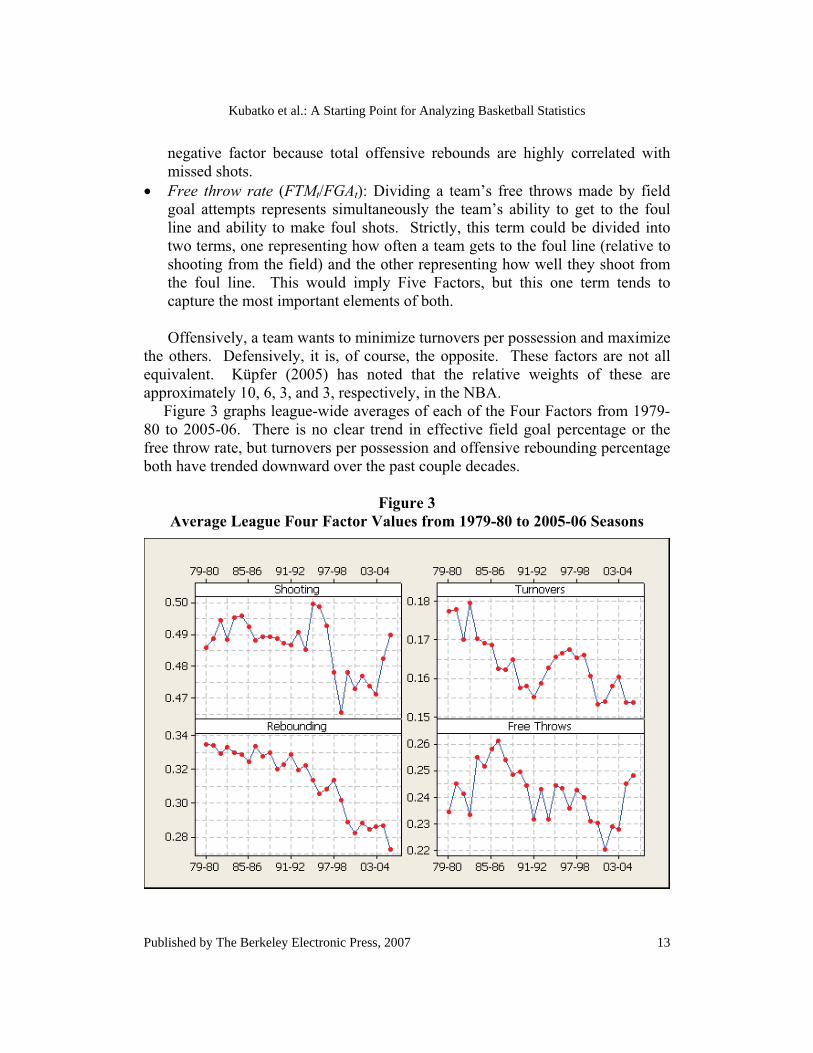
� Free throw rate (FTMt/FGAt): Dividing a team’s free throws made by field goal attempts represents simultaneously the team’s ability to get to the foul line and ability to make foul shots. Strictly, this term could be divided into two terms, one representing how often a team gets to the foul line (relative to shooting from the field) and the other representing how well they shoot from the foul line. This would imply Five Factors, but this one term tends to capture the most important elements of both.

Offensively, a team wants to minimize turnovers per possession and maximize the others. Defensively, it is, of course, the opposite. These factors are not all equivalent. Küpfer (2005) has noted that the relative weights of these are approximately 10, 6, 3, and 3, respectively, in the NBA. Figure 3 graphs league-wide averages of each of the Four Factors from 1979-80 to 2005-06. There is no clear trend in effective field goal percentage or the free throw rate, but turnovers per possession and offensive rebounding percentage both have trended downward over the past couple decades.

Figure 3 Average League Four Factor Values from 1979-80 to 2005-06 Seasons

13



Plus/Minus Statistics

The National Hockey League has long tracked how well a player’s team does while he is on the ice. This is called a “plus/minus statistic.” In the NBA, tracking this statistic has been made possible only recently thanks to the availability of play-by-play data on the Internet. In particular, 82games.com began collecting and posting this information for many players beginning in 2003. Prior to 82games.com, Harvey Pollack of the Philadelphia 76ers began collecting this information in 1993-94 and published total plus/minus for each player in his annual statistical handbook (Pollack, various years). Note that “plus/minus” is often used interchangeably for somewhat different concepts, as described below.

� Plus/minus statistics measure the team point differential (offensive points minus defensive points or offensive rating minus defensive rating) when a particular player is in the game; plus/minus statistics are often measured on a per-minute or per-possession basis.

� Net plus/minus statistics measure the plus/minus statistics for a given player when that player is in the game relative to the plus/minus statistics for that team when that player is not in the game. This was once called “Roland Rating” by the founder of 82games.com, but that name is now used for a rating that includes net plus/minus and individual statistics.

� Adjusted plus/minus statistics account for differences across players in the quality of the teammates they play with and opponents they play against. A description of the general method is given in Rosenbaum (2004).

The biggest advantage of plus/minus statistics is that they account for a player's contributions that are not tracked by the box score. Setting effective picks, the ability to spread the floor, and playing good help defense are all examples of skills accounted for by plus/minus statistics that are not captured by individual player statistics. Plus/minus statistics measure how a team performs when a given player is on the floor, so they are, in essence, the individual player version, of the team efficiency differential (offensive rating minus defensiverating). The biggest disadvantage of most plus/minus statistics is that they confound a player’s performance with the performance of his four teammates while on the floor (and five opponents, as well). Net plus/minus statistics account for some of this issue by subtracting off how the team does without the player, effectively assuming that player substitutions are uncorrelated. However, strong correlations between teammates’ minutes on the court and systematic differences in the quality of the opponents different players face are not entirely accounted for using

14



net plus/minus statistics. Starting lineups often play a large number of minutes together, as do deep reserves. Adjusted plus/minus statistics use regression techniques to account for the players a given player plays with and against. First developed as WINVAL by Jeff Sagarin and Wayne Winston, Rosenbaum (2004) outlines the general method that relates team point differentials (or net efficiency ratings) to variables indicating whether a player is in the game (and on the home or away team). The coefficients on the player variables isolate the marginal contributions of those players, accounting for the contributions of their teammates and opponents. However, in general, it takes many games to get reasonably precise estimates for these coefficients.

Counterpart Statistics

Counterpart statistics for player A represent the statistics posted by the opposing team’s player at player A’s position. 82games.com has posted these statistics since 2003-04. Because positions are often not clearly defined and because cross-match-ups can occur, counterpart statistics have been considered difficult to interpret. These dangers are greatest when counterpart statistics are estimated from box score data. Estimating from play-by-play data is better, while using observers to chart games is the preferred way to collect these statistics.

Individual Possession Usage and Efficiency Statistics

Because possessions at a team level are so important for understanding team performance, it makes sense to consider them at an individual level. Oliver (2004) and Hollinger (2003) introduce the concept of an individual possession rate, which measures how intensively players use possessions through field goal attempts, free throw attempts, assists, turnovers, and (in the case of Oliver) offensive rebounds. Oliver also normalizes individual possession rates so that individual players (one fifth of the team on the floor at any given time), on average, use one fifth of the team’s possessions while they are on the floor. Oliver (2004) also introduces the concept of an individual offensive rating or individual offensive efficiency. The individual offensive rating is the individual-level version of the team offensive rating, and it measures how efficient players are with their possessions.18 Weighting by possession usage and minutes played, individual offensive ratings should add up to the team offensive rating. Thus, together individual possession rates and individual offensive ratings are a good way to decompose the team offensive rating; they also provide a framework for

18 See Oliver (2004) for full details on the computation of individual possession rates and individual offensive efficiency.

15



assessing the size of offensive roles played by players and how efficient they are in those roles. In addition, most basketball analysts argue that there is typically a tradeoff between possession usage and efficiency. In fact, many analysts would argue that this is the central optimization problem for a basketball team; Oliver (2004) provides an empirical example of such an optimization. Players use up their easy opportunities to score on dunks, lay-ups, and wide open shots. However, as they increase their possession usage beyond those shots (and assists), the quality of the opportunities fall. But they fall at different rates for different players. Moreover, teams adjust their defensive strategies to reduce the efficiency of the players most likely to be able to shoulder a higher possession rate. All of these factors have resulted in it being difficult to obtain conclusive evidence on the negative relationship between possession usage and efficiency (at least in publicly available studies). What is necessary is a credible instrument (something related to possession usage, but with no independent effect on efficiency) to isolate the relationship between possession usage and efficiency.

Linear Weights

The term linear weights represents a class of player valuation methods that are a weighted sum of player statistics. Many different forms exist, most of which were developed following logical approaches. The most basic form is that of the NBA’s efficiency statistic (NBA_EFFp), used on the NBA Web site (NBA.com, 2007), but also used by other practicioners:

� �19 _

_ _ .p p p p p p

p p p

NBA EFF PTS REB AST STL BLKTO Missed FG Missed FT

�

Other linear weights measures apply different weights to each of these terms; also, a player’s rebounds (REBp) can be broken down into offensive and defensive rebounds, each with different weights. A summary of many different linear weights formulations can be found in Oliver (2004). As pointed out by several authors, including Oliver (2004) and Berri et al. (2006), linear weights have numerous faults, including the frequently subjective weights applied to the statistics, the lack of defensive statistics available for such systems, the lack of correlation with winning at the team level, the theoretical difficulty in incorporating new statistics that may be developed, and the general lack of a measuring stick to calibrate their accuracy. Recent work by Berri et al. (2006) assumes the externalities that players provide their teammates are not important, which allows them to develop a linear

16



weights formulation by first determining the relationship between wins and team statistics and then assuming a similar relationship between wins and individual statistics. Rosenbaum (2004) uses regression to develop a linear weights approximation for his adjusted plus/minus estimates of player value. Besides these methods, the most prominent linear weights techniques include Player Efficiency Rating (PER) from John Hollinger (2003, 2004, and 2005), TENDEX from Dave Heeren (1988), and Points Created from Bob Bellotti (1994).

Pythagorean Winning Percentage

A Bill James invention in baseball, Pythagorean records are based on the knowledge that team winning percentages are generally closely related to points scored and points allowed (and, in cases where they differ, the difference is usually not a repeatable skill). The Pythagorean winning percentage (PYTHt) is formulated as

� �20 .xt

t x xt o

PTSPYTHPTS PTS

�

where the subscript t still indicates team, the subscript o indicates opponent, and the superscript x is an exponent that is empirically determined. In baseball, James (1985, e.g.) found empirically that x = 2, leading to the use of the term Pythagorean. Subsequent rigorous distributional work, especially by Miller (2006), found that a slightly lower exponent of around 1.8 works best. In NBA basketball, the value of x has been estimated empirically from different works to be between about 13 and 17 (see Oliver, 1996, CoolStandings, 2006, for example). The value varies both by the era and by how important the estimator has seen capturing the extremes. In particular, margins of victory have changed little over the last 30 years – even as the pace of the NBA slowed. This has resulted in smaller exponents being necessary to correlate points to winning percentage. But capturing the very good and very bad teams, of which there are only a few each season, is done much better with a larger exponent. Typical least-squares-type error estimates of the exponent tend to yield a smaller exponent because so many teams are bunched between about 30 and 50 wins (winning percentages between about 38% and 62%). But increasing the exponent to better capture very good and very bad teams does not significantly compromise those teams in the middle and, as such, Oliver has been joined by ESPN (2007) in the use of an exponent of 16.5. In other leagues, including college, high school and the WNBA, smaller exponents have been found to work better because there are fewer possessions in

17



the typical game in these leagues (see Pomeroy, 2006, for example). Also, note that because of the equality of possessions for a team and its opponents, PTSt and PTSo can be replaced in the above equation by ORtgt and DRtgt.

Bell Curve Method

The Bell Curve method (introduced in Oliver, 2004) is a relatively more theoretical approach to relating points scored and allowed to a team’s winning percentage. Unlike the Pythagorean method, the Bell Curve method is based on the assumption that the distributions for teams’ points scored and allowed are normally distributed and can be subtracted from each other to form another normally distributed random variable, net points. Net points are normalized by dividing by the standard deviation of net point for that specific team, thus forming a Z-statistic. The estimated probability of winning is then given by the probability that a random variable distributed standard normal takes on a value less than this Z-statistic. The formula for predicting winning percentage for team t(Win%t) using this method is:

� � � �21 % t o

t o

PPG PPGWin NORMSDISTStDev PPG PPG

� ��

� �� where PPGt is points per game for team t, PPGo is points per game for opponents o, StDev(PPGt – PPGo) is the standard deviation of net points (PPGt – PPGo)across a team’s schedule, and NORMSDIST is the normal cumulative distribution function and represents the area under the standard normal “bell curve” to the left of the value in brackets.19

As with the Pythagorean method, team points per game and points allowed per game values can be replaced with offensive and defensive ratings, along with their standard deviations. The benefits of the Bell Curve method over the Pythagorean method are that

� it does not need empirical modification for application in different leagues or different eras, and

� it incorporates information about how much teams play up or down to their opponents.

19 This is the NORMSDIST function in MS Excel. Note that individual game data on net points is necessary to apply the Bell Curve method. Note also that, because ties are not allowed in basketball, the denominator of the function above (representing the standard deviation of the team’s net points) incorporates extra noise as additional variance. This causes the method to be slightly biased towards 0.500 a little bit (about one to two percentage points) for teams that are far from 0.500.

18



It also has additional accuracy, but this difference is very slight and the simplicity of the Pythagorean method can often make it preferred.

4. Sources of Data for Basketball Statistics

The Web provides an array of sites with basketball data. Most people know about Web sites such as NBA.com (http://www.nba.com), ESPN.com (http://www.espn.com), and Yahoo! Sports (http://sports.yahoo.com). These sites provide daily coverage of the NBA, and their sites are constantly updated during the season with contemporary statistics, rosters, and schedules. Other than the big media sites, here are some other sites that we frequently use for historical and other contemporary information: 82games.com (http://www.82games.com): This site, which is run by Roland Beech, provides both modern analysis of the NBA using some of the techniques above, but also some data resources. The site uses detailed play-by-play data from 2002-03 through the (regularly updated) current season to examine questions such as (a) how the Lakers perform when Kobe Bryant is on the court as opposed to when he is off the court, (b) how opposing centers have performed when Yao Ming is on the court, (c) how teams shoot from different parts of the court or at different stages of the shot clock, (d) how teams have fared with different line-ups on the court, (e) how players have performed in clutch time, and much, much more. These play-by-play data fill in many of the gaps left by traditional box score statistics. The original play-by-play data is not available publicly on the 82games site, but in the past sufficiently original and interesting research plans have resulted in 82games providing some of its data to researchers. Beech takes requests from readers for “research projects,” providing them with data in return for articles written for the site. This can be a useful way to start research projects. APBRmetrics Forum (http://sonicscentral.com/apbrmetrics/): This discussion board is not a data source, per se, but it is an excellent resource for anyone interested in serious discussions about the statistical analysis of basketball. The site is run by Kevin Pelton, and is a descendant of the APBR_analysis group on Yahoo! Groups. Basketball-Reference.com (http://www.basketball-reference.com): An on-line basketball encyclopedia run by Justin Kubatko, this site is practically a one-stop shop for historical basketball statistics. This site includes regular season data for players, coaches and teams for the entire history of the NBA. Data from the playoffs and individual game box score data are available for an increasing number of years. The site is also rich with biographical data and even includes college statistics and salary information for many players. Also, much of the work by analysts such as John Hollinger and Dean Oliver has been incorporated

19



into the site. Finally, the site allows for queries of specific information, which can be very useful for research purposes. DatabaseBasketball.com (http://www.databasebasketball.com): This bare bones site provides zip files for download of NBA season stats for players and teams, including playoff data. It also has information on coaches. Some of this information is incorrect (so research using these data should be done with care), but these files provide a reasonable starting point for a personal database. Doug’s MLB and NBA Statistics (http://www.dougstats.com): Doug Steele’s site provides current season data in a form that is easily imported into most spreadsheet applications and is updated on a daily basis. Doug also provides historical NBA statistics dating back to the 1988-89 season. Kenpom.com (http://www.kenpom.com): Ken Pomeroy’s site provides data and analysis for college basketball. The site includes (among many other things) advanced statistics for both teams and players. Rodney Fort’s Sport Business Data page (http://www.rodneyfort.com/SportsData/BizFrame.htm): Fort has collected a treasure trove of historical financial, attendance, and winning percentage data for the NFL, NBA, NBA, and MLB.

5. Conclusion

The quantitative analysis of sports is a new branch of science and, in many ways one that has grown through non-academic and non-traditionally peer-reviewed work. The aim of this paper is to bring to a peer-reviewed journal the generally accepted basics of the analysis of basketball, thereby providing a common starting point for future research in basketball. The possession concept is central to this work. The concept of equal possessions for opponents in a game has been in the statistical community for approximately 20 years and has withstood substantial review and commentary. Possession estimates have existed for approximately two decades, but the various formulas have sometimes created confusion. We hope that by showing how most previous formulas are special cases of our more general formulation, we shed light on the relationship between possessions and various statistics. Also, we hope that our new estimates can provide a common basis for future possession estimation. Regardless, we suggest that the possession framework be considered in future basketball research, as it continues to get review from “peers” now working in the NBA. The other concepts and methods discussed above are by no means a comprehensive list of methodologies used in the field or even by the authors, but we believe that they provide a set of tools that fit within the possession framework and form the basis of common conversations on statistical research in basketball.

20



References

Bellotti, Bob. The Points Created Pro Basketball Book of 1993-94. 1994. Nightwork Publishing, New Brunswick, NJ.

Berri, David J., Martin B. Schmidt, and Stacey L. Brook. The Wages of Wins: Taking Measure of the Many Myths in Modern Sport. 2006. Stanford University Press, Stanford, CA: Stanford University Press,.

CoolStandings. “Do You Use the Bill James Pythagorean Theorem for Sports other than Baseball?” 2007. http://www.coolstandings.com/football/faq.asp?sn=2006#faq14, available as recently as 1/22/07.

ESPN.com. “2006-07 NBA Expected Winning Percentage.” 2007. http://sports.espn.go.com/nba/stats/rpi, available as recently as January 15, 2007.

Heeren, Dave. The Basketball Abstract. 1988. Prentice Hall, Englewood Cliffs, NJ, Prentice Hall.

Hollinger, John. Pro Basketball Forecast: 2004-05 Edition. 2004. Brassey’s, Washington, DC: Brassey’s.

-----. Pro Basketball Forecast: 2005-06 Edition. 2005. Brassey’s, Washington, DC: Brassey’s, 2005.

-----. Pro Basketball Prospectus: All-New 2003-04 Edition. 2003. Brassey’s, Washington, DC: Brassey’s.

James, Bill. The 1985 Baseball Abstract. Ballantine Books, 1985. Küpfer, Ed. “Team Similarity.” 2005. APBRMetrics forum,

http://www.sonicscentral.com/apbrmetrics/viewtopic.php?p=118&sid=ff925dbe120f6c6f86e596d0d6dabbb8.

McGuire, Frank. Defensive Basketball. 1959. Prentice Hall, Englewood Cliffs, NJ.

Miller, Stephen J. “A Derivation of the Pythagorean Won-Loss formula in Baseball,” Chance Magazine, forthcoming.

NBA.com. “Efficiency Statistics.” http://www.nba.com/statistics/efficiency.html, available as recently as January 19, 2007.

Oliver, Dean. Basketball on Paper. 2004. Brassey’s, Washington, DC. -----. “Established Methods.” 1996. Journal of Basketball Studies,

http://www.rawbw.com/~deano/methdesc.html#pyth.-----. “New Measurement Techniques and a Binomial Model of the Game of

Basketball.” 1991. Journal of Basketball Studies,http://www.rawbw.com/~deano/articles/bbalpyth.html.

Pollack, Harvey. Harvey Pollack’s NBA Statistical Yearbook. Various years.

21



Pomeroy, Ken. “Ratings Explanation.” 2007. Kenpom.com Blog,http://kenpom.com/blog/index.php/weblog/ratings_explanation/, available as recently as 1/22/07.

Rosenbaum, Dan T. “Measuring How NBA Players Help their Teams Win.” 2004. 82games.com, http://www.82games.com/comm30.htm.

22



Documents

-A Starting Point for Analyzing Basketball Statistics.pdf