, 3: 1-27 Study protocol for the evaluation of a …umu.diva-portal.org/smash/get/diva2:1089292/FULLTEXT01.pdf · In May 2011 the Swedish government commissioned the Public Employment

http://www.diva-portal.org

This is the published version of a paper published in .

Citation for the original published paper (version of record):

Fowler, P., de Luna, X., Johansson, P., Ornstein, P., Bill, S. et al. (2017)Study protocol for the evaluation of a vocational rehabilitation., 3: 1-27

Access to the published version may require subscription.

N.B. When citing this work, cite the original published paper.

Permanent link to this version:http://urn.kb.se/resolve?urn=urn:nbn:se:umu:diva-133847

Observational Studies 3 (2017) 1-27 Submitted 1/17; Published 4/17

Study protocol for the evaluation of a vocationalrehabilitation

Philip Fowler [email protected] of Statistics, USBE, Umea University, SE-90187 Umea, Sweden

Xavier de Luna [email protected] of Statistics, USBE, Umea University, SE-90187 Umea, Sweden

Per Johansson [email protected] of Statistics, Uppsala University, SE-75120 Uppsala, SwedenThe Institute for Evaluation of Labour Market and Education Policy, SE-75120 Uppsala, SwedenThe Institute for the Study of Labor IZA, Bonn, Germany

Petra Ornstein [email protected] Swedish Social Insurance Agency, SE-10351 Stockholm, Sweden

Sofia Bill [email protected] Swedish Social Insurance Agency, SE-10351 Stockholm, Sweden

Peje Bengtsson [email protected]

The Swedish Social Insurance Agency, SE-10351 Stockholm, Sweden

Abstract

This paper presents a study protocol for the evaluation of a vocational rehabilitation,namely a collaboration between the Swedish Social Insurance Agency and the Public Em-ployment Service, where individuals needing support to regain work ability were called toa joint assessment meeting. This protocol describes a matching study design using a lassoalgorithm, where we do not have access to outcome data on work ability for the treated.The matching design is based on a collection of health and socio-economic covariates mea-sured at baseline. We also have access to a prognosis made by caseworkers on the expectedlength of the individual sick leave. This prognosis variable is, we argue, a proxy variablefor potential unmeasured confounders. We present results showing balance achieved onobserved covariates.

Keywords: Love Plots, Matching Design, Observational Study, Proxy Variable

1. Introduction

In May 2011 the Swedish government commissioned the Public Employment Service (PES)and the Swedish Social Insurance Agency (SIA) to increase the effort and scope of theircooperation. The target group of the joint efforts were individuals entering sick leave and

c©2017 Philip Fowler, Xavier de Luna, Per Johansson, Petra Ornstein, Sofia Bill and Peje Bengtsson.

Fowler et al.

identified to need support in order to regain work ability. During 2012 the authoritiesimplemented a model for enhanced cooperation, with a method called joint assessment.

In a joint assessment meeting (JAM), the individual meets PES and SIA over one tomultiple meetings. Other agents such as caregivers, employers and the municipality maypartake. The aim of the assessment is to identify the individual’s work ability from a medicalas well as a labour market perspective. It is stressed that the individual should be active inthe planning and implementation of all interventions and that the authorities should workmethodically to stimulate and motivate the individual’s participation. Thus, for the sickleave cases, JAMs can lead to rehabilitation plans being formed.

The aim of this paper is to present a study protocol for the evaluation of the effect ofbeing called to a JAM on outcomes related to work ability. These outcomes are not observedfor those called to a JAM at the stage of designing the study presented here. Instead, theoutcomes will be retrieved from the data holder once this protocol is accepted for publicationand then the study described herein will be implemented and the results of the evaluationpublished. This guarantees that the study design presented here has not been influenced byseeing any treatment effect estimates as advocated by Rubin (e.g., Rubin, 2007). There arepotential costs in not using outcome observations to design an observational study since, forinstance, confounder selection yields more efficient treatment effect estimators when basedon observed outcomes (see, e.g., de Luna et al., 2011). However, this is arguably outweighedby the facts that not observing outcome data ensure that the design has not been geared(even unconsciously) towards a given result.

The paper is structured in accordance with the STROBE statement (von Elm et al.,2008). Section 2 describes the study design, the variables included in the study, and presentsa matching algorithm; see Stuart (2010) for a review of matching. The observational studydesign described has several novel aspects. It is based on a collection of health and socio-economic covariates measured at baseline, but we also have access to a prognosis madeby caseworkers on the expected length of the individual sick leave in the absence of a callto JAM. We argue that this prognosis variable may be considered as a proxy variable forpotential unmeasured confounders; see de Luna et al. (2017). Moreover, the matching designuses an algorithm based on lasso regression (Tibshirani, 1996) and a balancing stopping rulesimilar to work presented in Diamond and Sekhon (2013). Section 3 shows results describingbalance on observed covariates achieved by this matching design and briefly describes theevaluation study intended. Section 4 concludes the paper.

2

Study protocol for the evaluation of a vocational rehabilitation

2. Study design and method

2.1 Design assumptions

The design is based on the Neyman-Rubin potential outcomes framework (Neyman, 1923;Rubin, 1974; Holland, 1986). For each individual i, let Ti be a binary treatment indicatorsuch Ti = 1 if he/she is treated and Ti = 0 if untreated. Furthermore, let Y1i and Y0i be theoutcome an individual would have if treated and untreated respectively. The parameter ofinterest is the average treatment effect among the treated, τ t = E (Y1i − Y0i | Ti = 1). Fora discussion of this parameter, see Imbens and Wooldridge (2009). Its precise meaning is,however, clear only when treatment and control groups are defined, see Section 2.3.1.

We will use a matching estimator to nonparametrically estimate τ t, where the outcomeof treated individuals are compared to that of controls with similar values on observedcovariates. See Stuart (2010) for a review of matching and Abadie and Imbens (2006) for aformal definition of matching estimators.

A set of pretreatment covariates, Xi, are available for each individual. In order to makeinference about the effect of the treatment, we need to assume that whether or not anindividual is treated does not affect the outcome for any other individual, see Rubin (1980;1986). Furthermore, the following assumptions yield indentification of τ t.

Assumption 1 (Unconfoundedness)Y0i ⊥⊥ Ti |Xi.

Assumption 2 (Common support)Pr (Ti = 0 |Xi) > 0.

Unconfoundedness cannot be tested empirically and sensitivity analysis to deviation fromit will be carried out. Common support can be investigated empirically and is typicallyenforced in a matching design by discarding treated individuals which do not have closematches.

2.2 Setting and Participants

The study population consists of all individuals registered at the SIA with a sick leave spellstarting from April 2012 and reaching between 31 and 365 days some time during the periodOctober 1, 2012 to March 31, 2013, the latter henceforth referred to as the evaluation period(EP). To be eligible for inclusion in our study, an individual can not have been called toa JAM in a previous sick leave period registered at SIA during the past six months. ThatJAMs further back in time are not excluded is due to data not being available to us.

2.3 Variables

2.3.1 Treatment

The treatment studied in this paper is to be called to a JAM during the EP. It is theresponsibility of SIA to identify individuals who could regain capacity to work throughvocational rehabilitation. Since 2011, the path to vocational rehabilitation for individualson sick leave is JAM. Vocational rehabilitation aiming at improving individuals’ general

3

Fowler et al.

capacity for work is the joint responsibility of SIA and PES, and has been so historically. Thecooperation of the authorities was however increased 2011 and the design of the new strategyfor enhanced cooperation, with JAM as the starting point, was implemented simultaneouslyin the whole country.

At a JAM, individuals are assessed in terms of whether or not they are ready for inter-ventions from the PES. A person is considered ready if he/she is seen considered healthyenough to take part in vocational rehabilitation. The PES and the SIA are jointly respon-sible however the PES is responsible for the active interventions. The cooperation betweenthe PES and the SIA consists of follow-up meetings with the individual where results arediscussed and activities can be revised, added, or removed. It is stressed that the indi-vidual should formulate objectives and adjust activities jointly with caseworkers from bothauthorities.

The PES offers two types of active interventions, namely work preparatory interven-tions and work oriented interventions. Work preparatory interventions aim to prepare andempower the individual before participation in work oriented interventions. Work orientedinterventions may be offered directly following JAM or after a period with work preparatoryinterventions. Activities include mentoring, job search, and workplace training.

It should be noted that the services that PES offer are available to unemployed, regard-less of them being sick benefit recipients or not. Individuals with sick benefits but withouta JAM (the control group) could also register at the PES which would allow them to takepart in these active interventions. This requires being registered at the PES as searching fora job. This would mean that the individuals would immediately lose their sickness benefits.They could instead obtain unemployment benefits but since these benefits are always sub-stantially lower than the sickness benefits this scenario is highly unlikely. Notwithstanding,this study aims at estimating the effect of the joint effort by the two agencies on sick benefitrecipients, and not effects of different interventions within the PES.

Treatment assignment is done by each individual’s caseworker. These caseworkers aretrained to make decisions regarding eligibility to get access to sickness benefits. This trainingis a priority at the SIA and the process is monitored on a yearly basis, ending in a reportof how to make improvements. Thus while the decision of JAM assessment is at eachcaseworker’s discretion, and therefore might vary between caseworkers, it is expected to bebased on similar principles.

2.3.2 Waiting time

For each individual i, we measure the number of days his or her sick leave in an ongoingsick spell has lasted. We call this ”waiting time” and denote it wi. Because waiting timecontains information on individuals, the effect of treatment should be estimated conditionalon wi (de Luna and Johansson, 2010). Thus, we consider waiting time strata as follows:[31, 70), [70, 91), [91, 109), [109, 126), [126, 146), [146, 166), [166, 181), [181, 214), [214, 249),[249, 366). This partition was chosen by looking at the deciles of waiting times among thetreated who fulfilled our inclusion criteria. The partitioning was then modified slightly totake into account that the monitoring of sick leave changes when the sick spell exceeds 90,180 or 365 days. Treatment status is thus determined within each stratum of waiting time,with Ti = 1 if an individual was called to a JAM during that stratum and Ti = 0 if not

4


called during the stratum nor earlier during the sick leave spell. We thus assume that theassumptions of Section 2.1 hold within each waiting time stratum.

2.3.3 Outcome

The main outcome of interest is the total extent of sick leave (TESL) measured, in percent,at the end of the month that occurs k = 1, 2 . . . , 21 months after an individual was calledto a JAM. The choice of 21 months is due to data not being available to us further aheadin time, at the time of data requisition. For controls, the outcome is measured k monthsafter the individual had a waiting time equal to that of its matched treated individual, seeSection 2.4. That is, suppose an individual was called to a JAM during February 2013 aftera waiting time of 70 days. Then the outcome is TESL at the end of March 2013, April2013, etc. For its matched controls the outcome is TESL measured at the end of the monththat occurs k months plus 70 days after their case started. The outcome for those calledto a JAM some time during the EP (i.e. treated individuals) was not available to us whiledesigning this study.

The parameter of interest is the average treatment effect among those treated within awaiting time stratum, as contrasted with those not treated in that waiting time stratum,but possibly later on.

2.3.4 Prognosis

A prognosis of the duration of the sick leave (if untreated) is available, and this covariateis referred to as ”prognosis” in the sequel. This forecast was made by caseworkers at SIA,after telephone interviews with the individuals. The prognosis was not used by casework-ers in discussions with the individuals so the subjects were not aware of their prognosis.Furthermore, the caseworkers were informed that the prognosis variable would not be usedto evaluate their performance as caseworkers. Prognosis is measured as an ordinal variablewith five levels, namely: At most 90 days sick leave (Very Short), Longer than 90 days butat most 180 days (Short), Longer than 180 days but at most 365 days (Medium), Longerthan 365 days but less than 915 days (Long), and At risk of reaching 915 days in sick leave(Very Long). We find it plausible that unmeasured confounders (such as the individual’sown assessment of his or her situation) inferred by the interviewer are taken into accountwhen making the prognosis. The idea being here that an individual’s own assessment ofhis or her situation is likely to be a good predictor of the length of the sick leave, and thatthe prognosis made by the caseworker after a telephone interview with the individual cantake this into account. Treatment assignment is later done by a caseworker (in the majorityof the time the same one), who likely bases his or her decision on this prognosis. Theseideas have been formalised in de Luna et al. (2017), where the prognosis is called a proxyvariable. Then, given the following assumptions

Assumption 3 (Proxy assumption)

i) Y0i ⊥⊥ (Ti, Pi) | (Xi,U i),

ii) Ti ⊥⊥ U i | (Xi, Pi),

5

Fowler et al.

Assumption 4 (Support on Proxy)P (Ti = 0 |Xi, Pi) > 0,

where Xi is the observed covariates, U i any unobserved covariates, and Pi denotes theprognosis (proxy variable), it follows that Y0i ⊥⊥ T | (Xi, Pi) (de Luna et al., 2017, Proposi-tion 1) and hence τ t is identified when conditioning on (Xi, Pi), even if Assumption 1 doesnot hold.

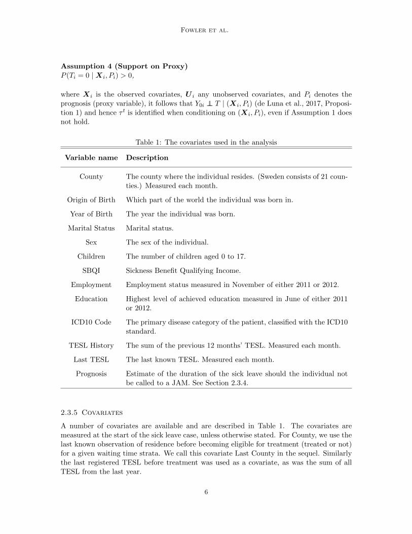
Table 1: The covariates used in the analysis

Variable name Description

County The county where the individual resides. (Sweden consists of 21 coun-ties.) Measured each month.

Origin of Birth Which part of the world the individual was born in.

Year of Birth The year the individual was born.

Marital Status Marital status.

Sex The sex of the individual.

Children The number of children aged 0 to 17.

SBQI Sickness Benefit Qualifying Income.

Employment Employment status measured in November of either 2011 or 2012.

Education Highest level of achieved education measured in June of either 2011or 2012.

ICD10 Code The primary disease category of the patient, classified with the ICD10standard.

TESL History The sum of the previous 12 months’ TESL. Measured each month.

Last TESL The last known TESL. Measured each month.

Prognosis Estimate of the duration of the sick leave should the individual notbe called to a JAM. See Section 2.3.4.

2.3.5 Covariates

A number of covariates are available and are described in Table 1. The covariates aremeasured at the start of the sick leave case, unless otherwise stated. For County, we use thelast known observation of residence before becoming eligible for treatment (treated or not)for a given waiting time strata. We call this covariate Last County in the sequel. Similarlythe last registered TESL before treatment was used as a covariate, as was the sum of allTESL from the last year.

6


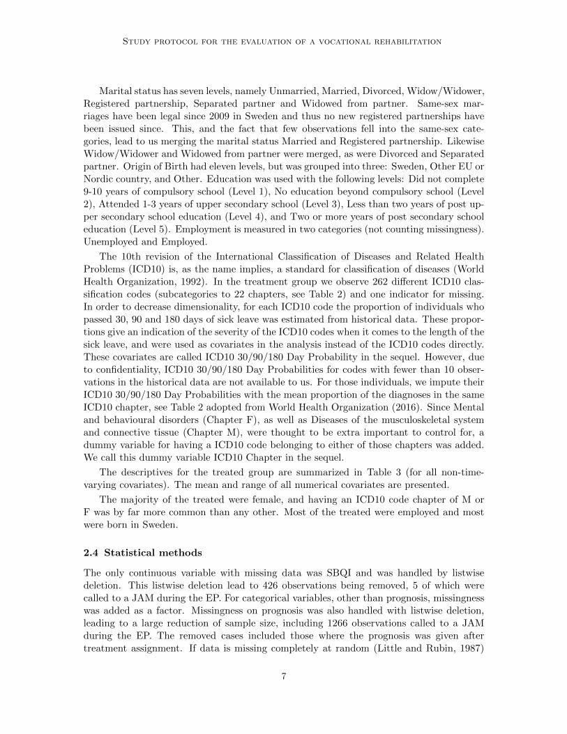
Marital status has seven levels, namely Unmarried, Married, Divorced, Widow/Widower,Registered partnership, Separated partner and Widowed from partner. Same-sex mar-riages have been legal since 2009 in Sweden and thus no new registered partnerships havebeen issued since. This, and the fact that few observations fell into the same-sex cate-gories, lead to us merging the marital status Married and Registered partnership. LikewiseWidow/Widower and Widowed from partner were merged, as were Divorced and Separatedpartner. Origin of Birth had eleven levels, but was grouped into three: Sweden, Other EU orNordic country, and Other. Education was used with the following levels: Did not complete9-10 years of compulsory school (Level 1), No education beyond compulsory school (Level2), Attended 1-3 years of upper secondary school (Level 3), Less than two years of post up-per secondary school education (Level 4), and Two or more years of post secondary schooleducation (Level 5). Employment is measured in two categories (not counting missingness).Unemployed and Employed.

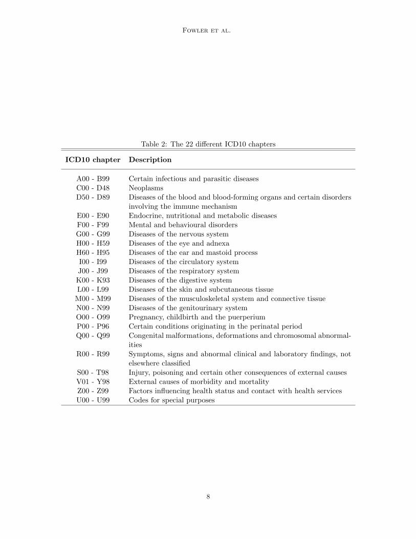
The 10th revision of the International Classification of Diseases and Related HealthProblems (ICD10) is, as the name implies, a standard for classification of diseases (WorldHealth Organization, 1992). In the treatment group we observe 262 different ICD10 clas-sification codes (subcategories to 22 chapters, see Table 2) and one indicator for missing.In order to decrease dimensionality, for each ICD10 code the proportion of individuals whopassed 30, 90 and 180 days of sick leave was estimated from historical data. These propor-tions give an indication of the severity of the ICD10 codes when it comes to the length of thesick leave, and were used as covariates in the analysis instead of the ICD10 codes directly.These covariates are called ICD10 30/90/180 Day Probability in the sequel. However, dueto confidentiality, ICD10 30/90/180 Day Probabilities for codes with fewer than 10 obser-vations in the historical data are not available to us. For those individuals, we impute theirICD10 30/90/180 Day Probabilities with the mean proportion of the diagnoses in the sameICD10 chapter, see Table 2 adopted from World Health Organization (2016). Since Mentaland behavioural disorders (Chapter F), as well as Diseases of the musculoskeletal systemand connective tissue (Chapter M), were thought to be extra important to control for, adummy variable for having a ICD10 code belonging to either of those chapters was added.We call this dummy variable ICD10 Chapter in the sequel.

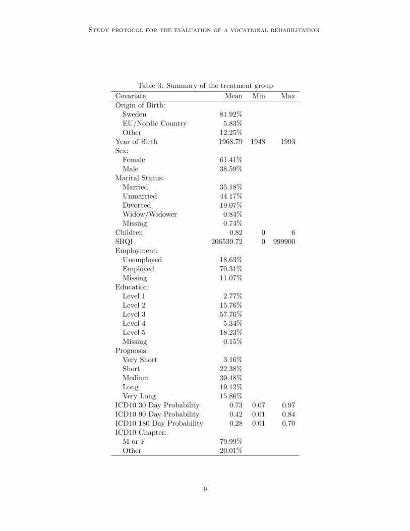
The descriptives for the treated group are summarized in Table 3 (for all non-time-varying covariates). The mean and range of all numerical covariates are presented.

The majority of the treated were female, and having an ICD10 code chapter of M orF was by far more common than any other. Most of the treated were employed and mostwere born in Sweden.

2.4 Statistical methods

The only continuous variable with missing data was SBQI and was handled by listwisedeletion. This listwise deletion lead to 426 observations being removed, 5 of which werecalled to a JAM during the EP. For categorical variables, other than prognosis, missingnesswas added as a factor. Missingness on prognosis was also handled with listwise deletion,leading to a large reduction of sample size, including 1266 observations called to a JAMduring the EP. The removed cases included those where the prognosis was given aftertreatment assignment. If data is missing completely at random (Little and Rubin, 1987)

7

Fowler et al.

Table 2: The 22 different ICD10 chapters

ICD10 chapter Description

A00 - B99 Certain infectious and parasitic diseasesC00 - D48 NeoplasmsD50 - D89 Diseases of the blood and blood-forming organs and certain disorders

involving the immune mechanismE00 - E90 Endocrine, nutritional and metabolic diseasesF00 - F99 Mental and behavioural disordersG00 - G99 Diseases of the nervous systemH00 - H59 Diseases of the eye and adnexaH60 - H95 Diseases of the ear and mastoid processI00 - I99 Diseases of the circulatory systemJ00 - J99 Diseases of the respiratory systemK00 - K93 Diseases of the digestive systemL00 - L99 Diseases of the skin and subcutaneous tissue

M00 - M99 Diseases of the musculoskeletal system and connective tissueN00 - N99 Diseases of the genitourinary systemO00 - O99 Pregnancy, childbirth and the puerperiumP00 - P96 Certain conditions originating in the perinatal periodQ00 - Q99 Congenital malformations, deformations and chromosomal abnormal-

itiesR00 - R99 Symptoms, signs and abnormal clinical and laboratory findings, not

elsewhere classifiedS00 - T98 Injury, poisoning and certain other consequences of external causesV01 - Y98 External causes of morbidity and mortalityZ00 - Z99 Factors influencing health status and contact with health servicesU00 - U99 Codes for special purposes

8


Table 3: Summary of the treatment group

Covariate Mean Min Max

Origin of Birth:Sweden 81.92%EU/Nordic Country 5.83%Other 12.25%

Year of Birth 1968.79 1948 1993Sex:

Female 61.41%Male 38.59%

Marital Status:Married 35.18%Unmarried 44.17%Divorced 19.07%Widow/Widower 0.84%Missing 0.74%

Children 0.82 0 6SBQI 206539.72 0 999900Employment:

Unemployed 18.63%Employed 70.31%Missing 11.07%

Education:Level 1 2.77%Level 2 15.76%Level 3 57.76%Level 4 5.34%Level 5 18.23%Missing 0.15%

Prognosis:Very Short 3.16%Short 22.38%Medium 39.48%Long 19.12%Very Long 15.86%

ICD10 30 Day Probability 0.73 0.07 0.97ICD10 90 Day Probability 0.42 0.01 0.84ICD10 180 Day Probability 0.28 0.01 0.70ICD10 Chapter:

M or F 79.99%Other 20.01%

9

Fowler et al.

for the treated and the missningness for the controls does not depend on the outcomeconditional on the covariates, listwise deletion does not bias the results of the analysis.If this assumption does not hold, then the estimator instead targets τ t defined on thepopulation of the non-missing.

In order to reduce the dimensionality of the matching problem, we estimate the prob-ability of being treated given the observed covariates, often referred to as the propensityscore. It can be shown (Rosenbaum and Rubin, 1983) that given Assumptions 1-2 (or 3-4)that τ t is identified conditional on the propensity score instead of on the covariates. Nearestneighbour propensity score matching with exact matching for additional key covariates wasperformed within each waiting time stratum. The covariates that were matched exactly onwere ICD10 Chapter, Prognosis and Sex, since prognosis is believed to be a proxy variablefor unmeasured confounders while ICD10 Chapter and Sex are considered key confounders.

Because the pool of controls is much larger than that of the treated, we perform afive-to-one matching to improve on efficiency. The goal of matching is to find treated andcontrols with similar distributions on covariates. One measure of similarity is the absolutestandardised mean difference between values of a covariate among the treated compared tothat of the controls. We refer to this as ”imbalance” in the sequel. The standardisation isdone by dividing each difference with the pooled pre matching standard deviation of thatcovariate. Thus a low average imbalance is a sign of the treated having similar distributionsof the covariates as the controls. To find a low average imbalance, matching was done inaccordance with Algorithm 1 below, similar in spirit to the genetic matching approach ofDiamond and Sekhon (2013).

Algorithm 1 Matching algorithm within a waiting time stratum.

Step 1. Run a large number of lasso regressions (Tibshirani, 1996) of treatment on thecovariates and their second order terms, excluding interactions with Last County,using the glmnet package (Friedman et al., 2010) in R (R Core Team, 2014), seedetails below.

Step 2. For each of the propensity score models fitted, perform 5-to-1 nearest neighbourmatching on the score, while matching also exactly on Sex, Prognosis and ICD10Chapter: M or F. The nearest neighbour matching is done with a caliper of within twostandard deviations. Treated individuals where 5 controls can not be found within thecaliper are discarded.

Step 3. For each propensity score matching performed in Step 2, calculate the imbalancefor each variable post matching. Calculate also the imbalance for each second-orderterm, excluding interactions with Last County, post matching. Store the matchingresults that lead to no more than 5 treated observations discarded.

Step 4. Of the matching results retained in Step 3, save the one that leads to the lowestaverage imbalance and discard the rest.

The lasso models were constructed with the glmnet function from the glmnet package inR, setting the control parameters nlambda, dfmax and lambda.min.ratio to 1000, 383 and0.001 respectively, with 383 being the number of second and first order terms available. This

10


resulted in between 716 and 845 lasso models being fitted in each waiting time stratum,with a maximum number of coefficients ranging from 231 to 283. The models selected byAlgorithm 1 had between 22 and 158 non-zero coefficients, with a mean of 88.9.

The exclusion of interactions with Last County in Steps 1 and 3 is due to its inclusionresulting in a very large increase in the number of terms in the lasso regression as well aseffectively giving Last County a much higher weight than the other covariates when checkingimbalance.

Bounding the maximum number of discarded treated in Step 3 is done to not favourmodels with a high number of unmatched treated since low post matching imbalance canbe achieved by choosing a propensity score model that matches few treated very well anddiscards the rest.

3. Results

3.1 Participants

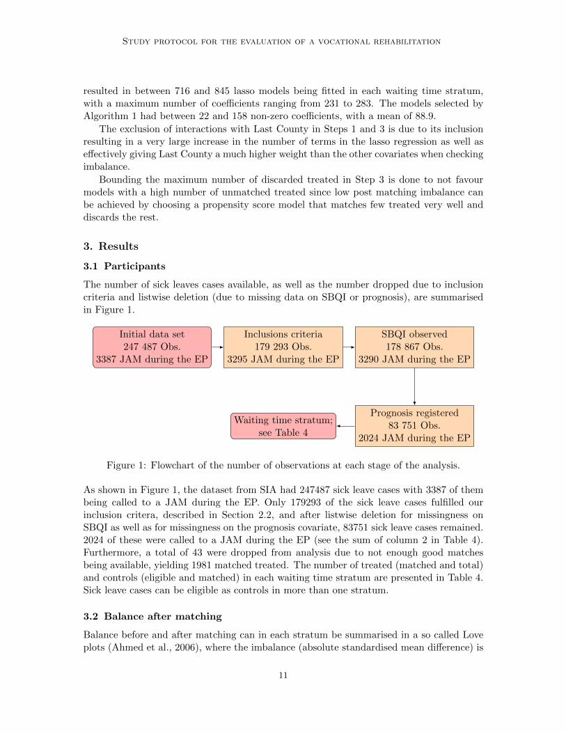
The number of sick leaves cases available, as well as the number dropped due to inclusioncriteria and listwise deletion (due to missing data on SBQI or prognosis), are summarisedin Figure 1.

Initial data set247 487 Obs.

3387 JAM during the EP

Inclusions criteria179 293 Obs.


SBQI observed178 867 Obs.


Prognosis registered83 751 Obs.


Waiting time stratum;see Table 4

Figure 1: Flowchart of the number of observations at each stage of the analysis.

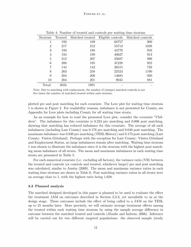
As shown in Figure 1, the dataset from SIA had 247487 sick leave cases with 3387 of thembeing called to a JAM during the EP. Only 179293 of the sick leave cases fulfilled ourinclusion critera, described in Section 2.2, and after listwise deletion for missingness onSBQI as well as for missingness on the prognosis covariate, 83751 sick leave cases remained.2024 of these were called to a JAM during the EP (see the sum of column 2 in Table 4).Furthermore, a total of 43 were dropped from analysis due to not enough good matchesbeing available, yielding 1981 matched treated. The number of treated (matched and total)and controls (eligible and matched) in each waiting time stratum are presented in Table 4.Sick leave cases can be eligible as controls in more than one stratum.

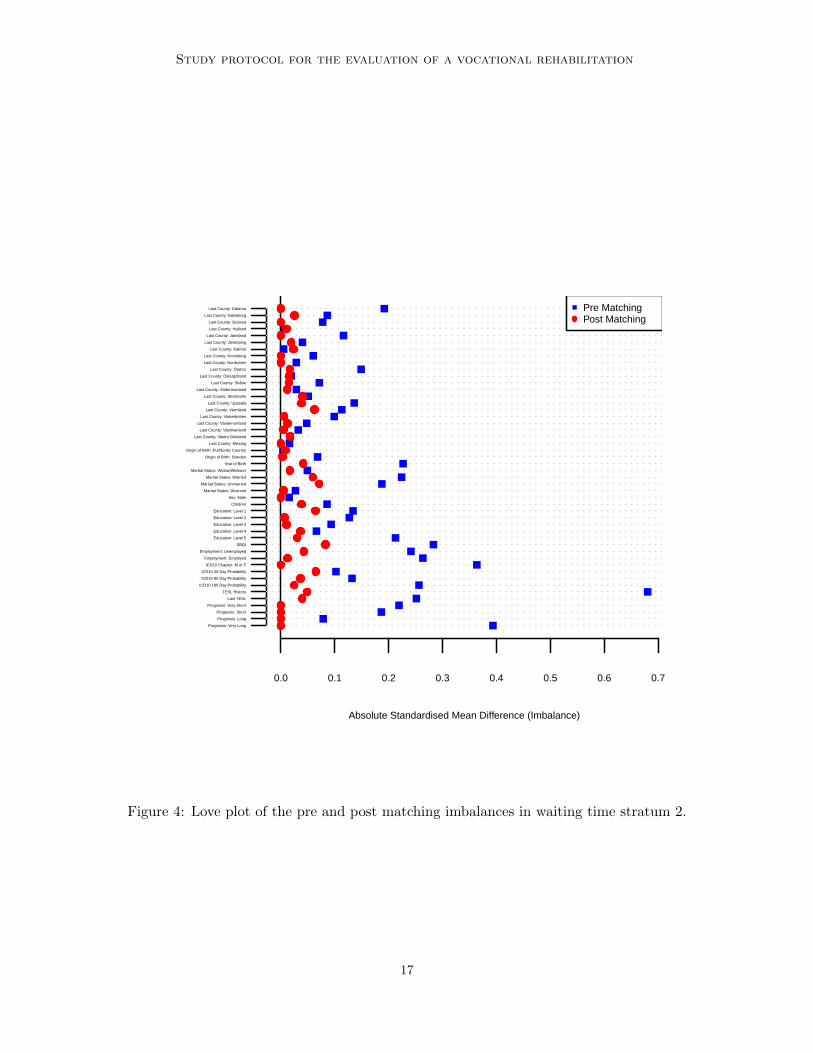
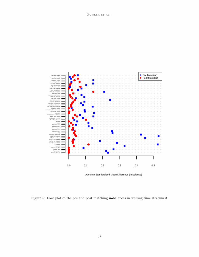
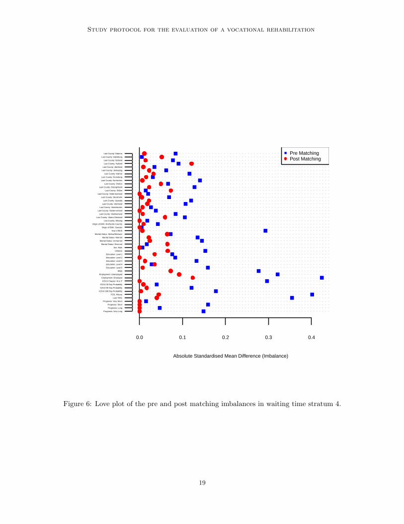
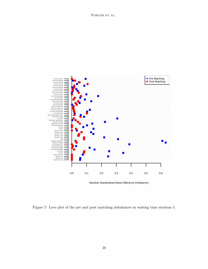
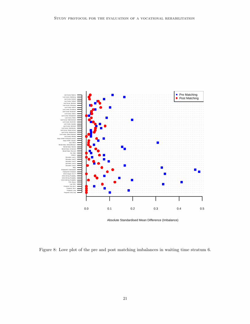
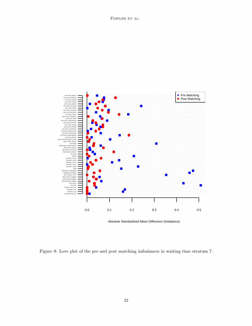
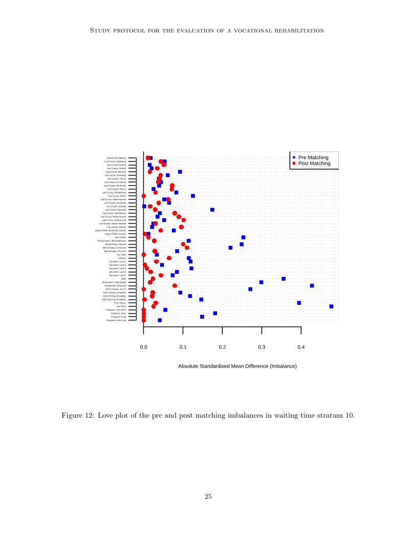
3.2 Balance after matching

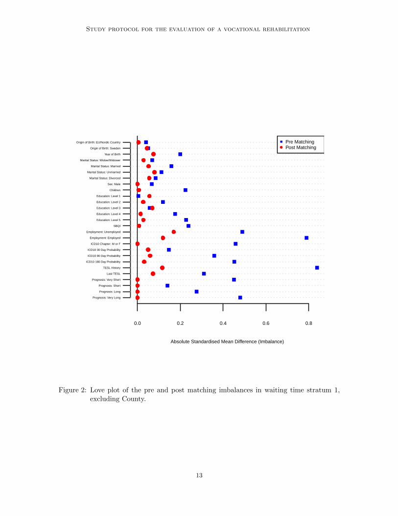
Balance before and after matching can in each stratum be summarised in a so called Loveplots (Ahmed et al., 2006), where the imbalance (absolute standardised mean difference) is

11

Fowler et al.

Table 4: Number of treated and controls per waiting time stratum

Stratum Treated Matched treated Eligible controls Matched controls

1 193 189 68757 9002 217 212 55713 10383 193 188 44770 9164 194 189 40627 9135 212 207 35687 9966 200 195 31228 9227 144 142 26515 7288 263 258 22524 11909 204 200 14685 920

10 204 201 9045 881

Total: 2024 1981 - -

Note: Due to matching with replacement, the number of (unique) matched controls is notfive times the number of matched treated within each stratum.

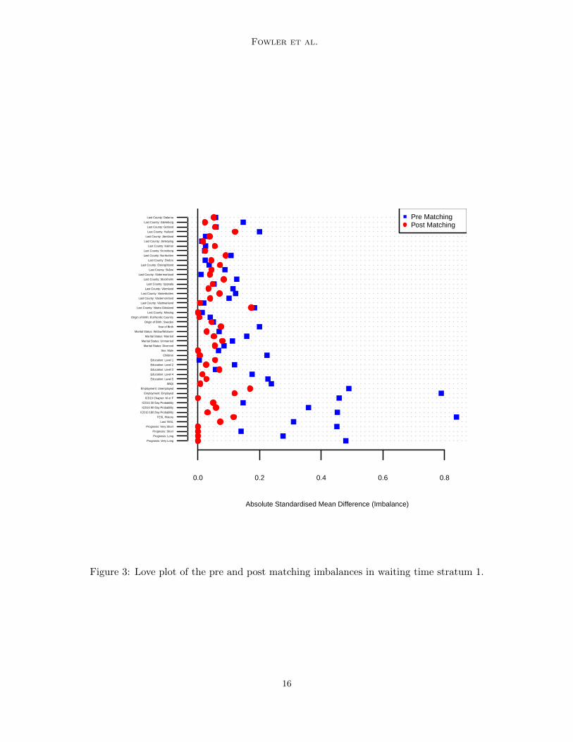
plotted pre and post matching for each covariate. The Love plot for waiting time stratum1 is shown in Figure 2. For readability reasons, imbalance is not presented for County, seeAppendix for Love plots including County for all waiting time strata.

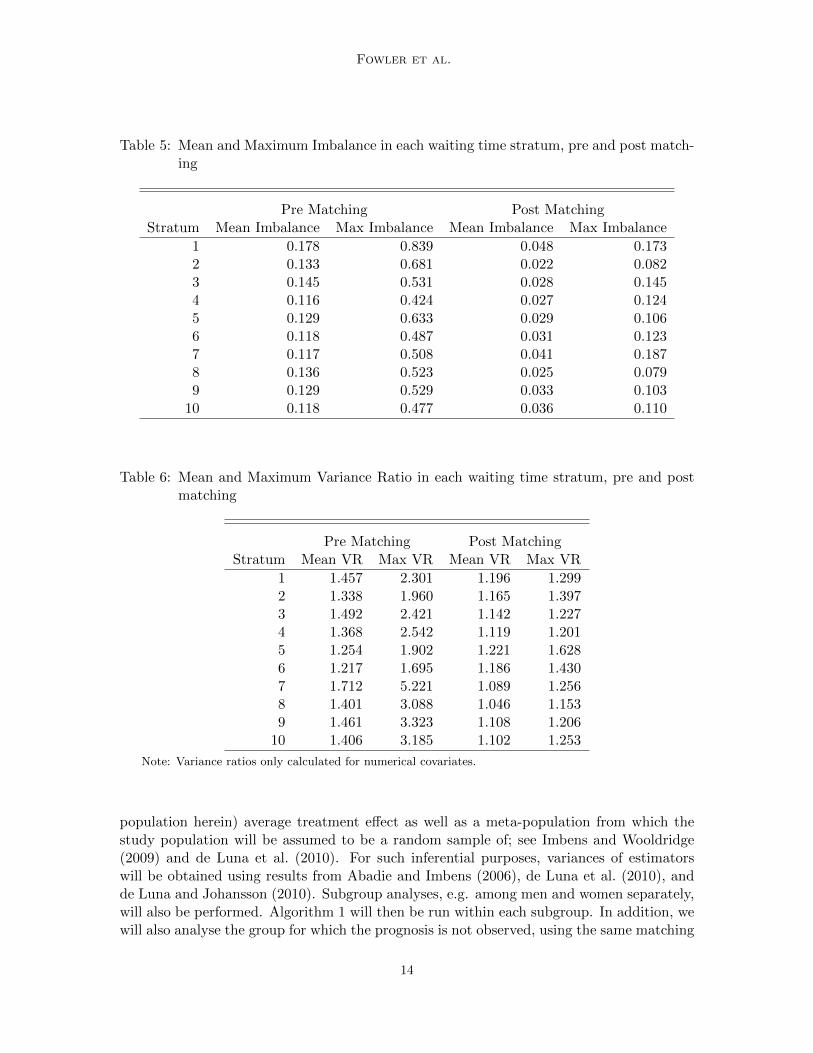
As an example for how to read the presented Love plot, consider the covariate ”Chil-dren”. The imbalance for this covariate is 0.224 pre matching and 0.006 post matching,showing that matching has reduced imbalance for this covariate. The average of all suchimbalances (including Last County) was 0.178 pre matching and 0.048 post matching. Themaximum imbalance was 0.839 pre matching (TESL History) and 0.173 post matching (LastCounty: Vastra Gotaland). Perhaps with the exception for Last County: Vastra Gotalandand Employment Status, no large imbalances remain after matching. Waiting time stratum1 was chosen to illustrate the imbalance since it is the stratum with the highest post match-ing mean imbalance of all strata. The mean and maximum imbalances in each waiting timestrata are presented in Table 5.

For each numerical covariate (i.e. excluding all factors), the variance ratio (VR) betweenthe treated and controls (or controls and treated, whichever larger) pre and post matchingwas calculated, similar to Austin (2009). The mean and maximum variance ratios in eachwaiting time stratum are shown in Table 6. Post matching variance ratios in all strata wereon average close to 1, with the highest ratio being 1.628.

3.3 Planned analysis

The matched designed developed in this paper is planned to be used to evaluate the effectthe treatment JAM on outcomes described in Section 2.3.3, yet unvailable to us at thedesign stage. These outcomes include the effect of being called to a JAM on the TESLup to 21 months later. More precisely, we will estimate average treatment effects amongthe treated within each waiting time stratum by using the sample average difference inoutcome between the matched treated and controls (Abadie and Imbens, 2006). Inferencewill be carried out for two different targeted populations: the observed sample (study

12


Absolute Standardised Mean Difference (Imbalance)

0.0 0.2 0.4 0.6 0.8

Prognosis: Very Long

Prognosis: Long

Prognosis: Short

Prognosis: Very Short

Last TESL

TESL History

ICD10 180 Day Probability



ICD10 Chapter: M or F

Employment: Employed

Employment: Unemployed

SBQI

Education: Level 5

Education: Level 4

Education: Level 3

Education: Level 2

Education: Level 1

Children

Sex: Male

Marital Status: Divorced

Marital Status: Unmarried

Marital Status: Married

Marital Status: Widow/Widower

Year of Birth

Origin of Birth: Sweden

Origin of Birth: EU/Nordic Country Pre Matching Post Matching

Figure 2: Love plot of the pre and post matching imbalances in waiting time stratum 1,excluding County.

13

Fowler et al.

Table 5: Mean and Maximum Imbalance in each waiting time stratum, pre and post match-ing

Pre Matching Post MatchingStratum Mean Imbalance Max Imbalance Mean Imbalance Max Imbalance

1 0.178 0.839 0.048 0.1732 0.133 0.681 0.022 0.0823 0.145 0.531 0.028 0.1454 0.116 0.424 0.027 0.1245 0.129 0.633 0.029 0.1066 0.118 0.487 0.031 0.1237 0.117 0.508 0.041 0.1878 0.136 0.523 0.025 0.0799 0.129 0.529 0.033 0.103

10 0.118 0.477 0.036 0.110

Table 6: Mean and Maximum Variance Ratio in each waiting time stratum, pre and postmatching

Pre Matching Post MatchingStratum Mean VR Max VR Mean VR Max VR

1 1.457 2.301 1.196 1.2992 1.338 1.960 1.165 1.3973 1.492 2.421 1.142 1.2274 1.368 2.542 1.119 1.2015 1.254 1.902 1.221 1.6286 1.217 1.695 1.186 1.4307 1.712 5.221 1.089 1.2568 1.401 3.088 1.046 1.1539 1.461 3.323 1.108 1.206

10 1.406 3.185 1.102 1.253

Note: Variance ratios only calculated for numerical covariates.

population herein) average treatment effect as well as a meta-population from which thestudy population will be assumed to be a random sample of; see Imbens and Wooldridge(2009) and de Luna et al. (2010). For such inferential purposes, variances of estimatorswill be obtained using results from Abadie and Imbens (2006), de Luna et al. (2010), andde Luna and Johansson (2010). Subgroup analyses, e.g. among men and women separately,will also be performed. Algorithm 1 will then be run within each subgroup. In addition, wewill also analyse the group for which the prognosis is not observed, using the same matching

14


design (without the prognosis variable) but keeping in mind that unmeasured confoundersthere could be of bigger concern due to the lack of prognosis variable.

Finally, sensitivity analysis to untestable assumptions is an important component inevaluation studies based on observational data, and we will focus on the unconfoundednessassumptions made, also in relation to the prognosis variable used as proxy.

4. Discussion

The aim of this paper was to present a study protocol for the evaluation of the effect of beingcalled to a joint assessment on outcomes related to work ability. Thus, we have developedand described a study design based on lasso regression and matching. Love plots wereused to describe the balance in observed pretreatment covariates, pre and post matching.While the design yields balanced observed covariates, this is an observational study withthe usual limitations in this context. In particular, one cannot discard the possibility thatunobserved confounders are not balanced. However, as an attempt to improve on this, weuse a prognosis of expected sick leave duration made by caseworkers as a proxy variablefor unobserved covariates, and thus the study design presented where prognosis is matchedfor is expected to balance also such unobserved heterogeneity. This proxy property ishowever not empirically testable and a sensitivity analysis will be carried out as part of theevaluation study planned. The latter study, when implemented, will yield an estimation ofthe effect of the joint assessment for those actually being called to the assessment duringthe evaluation period (the treated population). Generalisability of the results to otherpopulations may not necessarily be granted, for instance, if future treated populationsdiffer greatly in characteristics which modify the effect of the treatment.

Acknowledgments

We are grateful to Ingeborg Waernbaum, two anonymous reviewers and the associate editorfor helpful comments that have improved the paper. We acknowledge funding from theSwedish Social Insurance Agency. This study has been ethically vetted by the regionalethical review board in Umea.

Appendix

Below we present Love plots for the imbalance in each of the ten waiting time strata.

15

Fowler et al.


0.0 0.2 0.4 0.6 0.8


Prognosis: Long

Prognosis: Short


Last TESL

TESL History







SBQI

Education: Level 5

Education: Level 4

Education: Level 3

Education: Level 2

Education: Level 1

Children

Sex: Male





Year of Birth


Origin of Birth: EU/Nordic Country

Last County: Missing

Last County: Västra Götaland

Last County: Västmanland

Last County: Västernorrland

Last County: Västerbotten

Last County: Värmland

Last County: Uppsala

Last County: Stockholm

Last County: Södermanland

Last County: Skåne

Last County: Östergötland

Last County: Örebro

Last County: Norrbotten

Last County: Kronoberg

Last County: Kalmar

Last County: Jönköping

Last County: Jämtland

Last County: Halland

Last County: Gotland

Last County: Gävleborg

Last County: Dalarna Pre Matching Post Matching

Figure 3: Love plot of the pre and post matching imbalances in waiting time stratum 1.

16



0.0 0.1 0.2 0.3 0.4 0.5 0.6 0.7


Prognosis: Long

Prognosis: Short


Last TESL

TESL History







SBQI

Education: Level 5

Education: Level 4

Education: Level 3

Education: Level 2

Education: Level 1

Children

Sex: Male





Year of Birth












Last County: Skåne





Last County: Kalmar








17

Fowler et al.


0.0 0.1 0.2 0.3 0.4 0.5


Prognosis: Long

Prognosis: Short


Last TESL

TESL History







SBQI

Education: Level 5

Education: Level 4

Education: Level 3

Education: Level 2

Education: Level 1

Children

Sex: Male





Year of Birth












Last County: Skåne





Last County: Kalmar








18



0.0 0.1 0.2 0.3 0.4


Prognosis: Long

Prognosis: Short


Last TESL

TESL History







SBQI

Education: Level 5

Education: Level 4

Education: Level 3

Education: Level 2

Education: Level 1

Children

Sex: Male





Year of Birth












Last County: Skåne





Last County: Kalmar








19

Fowler et al.


0.0 0.1 0.2 0.3 0.4 0.5 0.6


Prognosis: Long

Prognosis: Short


Last TESL

TESL History







SBQI

Education: Level 5

Education: Level 4

Education: Level 3

Education: Level 2

Education: Level 1

Children

Sex: Male





Year of Birth












Last County: Skåne





Last County: Kalmar








20



0.0 0.1 0.2 0.3 0.4 0.5


Prognosis: Long

Prognosis: Short


Last TESL

TESL History







SBQI

Education: Level 5

Education: Level 4

Education: Level 3

Education: Level 2

Education: Level 1

Children

Sex: Male





Year of Birth












Last County: Skåne





Last County: Kalmar








21

Fowler et al.


0.0 0.1 0.2 0.3 0.4 0.5


Prognosis: Long

Prognosis: Short


Last TESL

TESL History







SBQI

Education: Level 5

Education: Level 4

Education: Level 3

Education: Level 2

Education: Level 1

Children

Sex: Male





Year of Birth












Last County: Skåne





Last County: Kalmar








22



0.0 0.1 0.2 0.3 0.4 0.5


Prognosis: Long

Prognosis: Short


Last TESL

TESL History







SBQI

Education: Level 5

Education: Level 4

Education: Level 3

Education: Level 2

Education: Level 1

Children

Sex: Male





Year of Birth












Last County: Skåne





Last County: Kalmar








23

Fowler et al.


0.0 0.1 0.2 0.3 0.4 0.5


Prognosis: Long

Prognosis: Short


Last TESL

TESL History







SBQI

Education: Level 5

Education: Level 4

Education: Level 3

Education: Level 2

Education: Level 1

Children

Sex: Male





Year of Birth












Last County: Skåne





Last County: Kalmar








24



0.0 0.1 0.2 0.3 0.4


Prognosis: Long

Prognosis: Short


Last TESL

TESL History







SBQI

Education: Level 5

Education: Level 4

Education: Level 3

Education: Level 2

Education: Level 1

Children

Sex: Male





Year of Birth












Last County: Skåne





Last County: Kalmar








25

Fowler et al.

References

Abadie, A. and Imbens, G. W. (2006). Large sample properties of matching estimators foraverage treatment effects. Econometrica, 74(1):235–267.

Ahmed, A., Husain, A., Love, T. E., Gambassi, G., Dell’Italia, L. J., Francis, G. S., Gheo-rghiade, M., Allman, R. M., Meleth, S., and Bourge, R. C. (2006). Heart failure, chronicdiuretic use, and increase in mortality and hospitalization: an observational study usingpropensity score methods. European Heart Journal, 27(12):1431–1439.

Austin, P. C. (2009). Balance diagnostics for comparing the distribution of baseline co-variates between treatment groups in propensity-score matched samples. Statistics inmedicine, 28(25):3083–3107.

de Luna, X., Fowler, P., and Johansson, P. (2017). Proxy variables for indentification ofcausal effects. Economics Letters, 150:152–154.

de Luna, X. and Johansson, P. (2010). Non-parametric inference for the effect of a treatmenton survival times with application in the health and social sciences. Journal of StatisticalPlanning and Inference, 140(7):2122–2137.

de Luna, X., Johansson, P., and Sjostedt-de Luna, S. (2010). Bootstrap inference for k-nearest neighbour matching estimators. IZA Discussion Papers 5361, Institute for theStudy of Labor, Bonn.

de Luna, X., Waernbaum, I., and Richardson, T. S. (2011). Covariate selection for thenonparametric estimation of an average treatment effect. Biometrika, 98(4):861–875.

Diamond, A. and Sekhon, J. S. (2013). Genetic matching for estimating causal effects:A general multivariate matching method for achieving balance in observational studies.Review of Economics and Statistics, 95(3):932–945.

Friedman, J., Hastie, T., and Tibshirani, R. (2010). Regularization paths for generalizedlinear models via coordinate descent. Journal of Statistical Software, 33(1):1–22.

Holland, P. W. (1986). Statistics and causal inference. Journal of the American StatisticalAssociation, 81(396):945–960.

Imbens, G. W. and Wooldridge, J. M. (2009). Recent developments in the econometrics ofprogram evaluation. Journal of economic literature, 47(1):5–86.

Little, R. J. and Rubin, D. B. (1987). Statistical analysis with missing data. John Wiley &Sons.

Neyman, J. (1923). Sur les applications de la theorie des probabilites aux experiencesagricoles: Essai des principes. Roczniki Nauk Rolniczych, X:1–51. In Polish, Englishtranslation by Dabrowska D. and Speed T. in Statistical Science, 5: 465–472, 1990.

R Core Team (2014). R: A Language and Environment for Statistical Computing. RFoundation for Statistical Computing, Vienna, Austria. Available from: http://www.R-project.org/.

26


Rosenbaum, P. R. and Rubin, D. B. (1983). The central role of the propensity score inobservational studies for causal effects. Biometrika, 70(1):41–55.

Rubin, D. B. (1974). Estimating causal effects of treatments in randomized and nonran-domized studies. Journal of Educational Psychology, 66(5):688–701.

Rubin, D. B. (1980). Randomization analysis of experimental data: The Fisher randomiza-tion test comment. Journal of the American Statistical Association, 75(371):591–593.

Rubin, D. B. (1986). Comment: Which ifs have causal answers. Journal of the AmericanStatistical Association, 81(396):961–962.

Rubin, D. B. (2007). The design versus the analysis of observational studies for causaleffects: parallels with the design of randomized trials. Statistics in medicine, 26(1):20–36.

Stuart, E. A. (2010). Matching methods for causal inference: A review and a look forward.Statistical Science, 25(1):1–21.

Tibshirani, R. (1996). Regression shrinkage and selection via the lasso. Journal of the RoyalStatistical Society. Series B (Methodological), 58(1):267–288.

von Elm, E., Altman, D. G., Egger, M., Pocock, S. J., Gøtzsche, P. C., and Vandenbroucke,J. P. (2008). The strengthening the reporting of observational studies in epidemiology(STROBE) statement: guidelines for reporting observational studies. Journal of ClinicalEpidemiology, 61(4):344 – 349.

World Health Organization (1992). The ICD-10 Classification of Mental and BehaviouralDisorders: Clinical descriptions and diagnostic guidelines. Geneva: World Health Orga-nization.

World Health Organization (2016). International statistical clas-sification of diseases and related health problems 10th revision.http://apps.who.int/classifications/icd10/browse/2016/en [Accessed 31 Dec 2016].

27

Documents

, 3: 1-27 Study protocol for the evaluation of a …umu.diva-portal.org/smash/get/diva2:1089292/FULLTEXT01.pdf · In May 2011 the Swedish government commissioned the Public Employment