warwick.ac.uk/lib-publicationswrap.warwick.ac.uk/93620/1/WRAP_Theses_Spooner_2017.pdf · 2.4 Phosphorus reaction: Thermodynamics and Kinetics . . . . . . . . . 14 ... Chapter 5 Calculating

warwick.ac.uk/lib-publications

A Thesis Submitted for the Degree of PhD at the University of Warwick

Permanent WRAP URL:

http://wrap.warwick.ac.uk/93620

Copyright and reuse:

This thesis is made available online and is protected by original copyright.

Please scroll down to view the document itself.

Please refer to the repository record for this item for information to help you to cite it.

Our policy information is available from the repository home page.

For more information, please contact the WRAP Team at: [email protected]

http://go.warwick.ac.uk/lib-publications

http://wrap.warwick.ac.uk/93620

mailto:[email protected]

Quantifying the Transient Interfacial

Area During Slag-Metal Reactions

Stephen R. A. Spooner

A thesis submitted in partial fulfilment of the requirements for the degree of

Doctor of Philosophy in Engineering

University of Warwick

Warwick Manufacturing Group

January 2017

Contents

List of Figures v

List of Tables xi

Acknowledgments xiii

Declaration xvi

Chapter 1 Introduction 1

1.1 Objectives of Study . . . . . . . . . . . . . . . . . . . . . . . . . . . . 3

1.2 Thesis Structure . . . . . . . . . . . . . . . . . . . . . . . . . . . . . 4

Chapter 2 Underpinning Knowledge 6

2.1 Modern History of the Steel Industry . . . . . . . . . . . . . . . . . . 6

2.2 The Integrated Steel Plant . . . . . . . . . . . . . . . . . . . . . . . . 7

2.2.1 Coke Making . . . . . . . . . . . . . . . . . . . . . . . . . . . 7

2.2.2 Ironmaking . . . . . . . . . . . . . . . . . . . . . . . . . . . . 8

2.2.3 Basic Oxygen Steelmaking . . . . . . . . . . . . . . . . . . . . 9

2.2.4 Steel Forming and Finishing . . . . . . . . . . . . . . . . . . . 10

2.3 The Basic Oxygen Furnace . . . . . . . . . . . . . . . . . . . . . . . 11

2.3.1 Further Dephosphorization Technologies . . . . . . . . . . . . 13

2.4 Phosphorus reaction: Thermodynamics and Kinetics . . . . . . . . . 14

2.5 The Interfacial Area of reaction within the Emulsion . . . . . . . . . 17

2.5.1 Droplet Size Distribution . . . . . . . . . . . . . . . . . . . . 17

2.5.2 Droplet Generation . . . . . . . . . . . . . . . . . . . . . . . . 20

2.5.3 Residence Time . . . . . . . . . . . . . . . . . . . . . . . . . . 21

2.5.4 Spontaneous Emulsification . . . . . . . . . . . . . . . . . . . 21

i

2.6 Unresolved Findings from the Literature . . . . . . . . . . . . . . . . 23

Chapter 3 Formulating the Research Approach 25

3.1 Hypotheses . . . . . . . . . . . . . . . . . . . . . . . . . . . . . . . . 25

3.1.1 Hypothesis 1 . . . . . . . . . . . . . . . . . . . . . . . . . . . 25

3.1.2 Hypothesis 2 . . . . . . . . . . . . . . . . . . . . . . . . . . . 26

3.1.3 Hypothesis 3 . . . . . . . . . . . . . . . . . . . . . . . . . . . 26

3.1.4 Hypothesis 4 . . . . . . . . . . . . . . . . . . . . . . . . . . . 26

3.1.5 Hypothesis 5 . . . . . . . . . . . . . . . . . . . . . . . . . . . 27

3.1.6 Hypothesis 6 . . . . . . . . . . . . . . . . . . . . . . . . . . . 27

3.1.7 Hypothesis 7 . . . . . . . . . . . . . . . . . . . . . . . . . . . 27

3.2 Hypothesis Approach . . . . . . . . . . . . . . . . . . . . . . . . . . . 27

3.2.1 Hypothesis 1 . . . . . . . . . . . . . . . . . . . . . . . . . . . 27

3.2.2 Hypothesis 2 . . . . . . . . . . . . . . . . . . . . . . . . . . . 28

3.2.3 Hypothesis 3 & 4 . . . . . . . . . . . . . . . . . . . . . . . . . 28

3.2.4 Hypothesis 5 . . . . . . . . . . . . . . . . . . . . . . . . . . . 28

3.2.5 Hypothesis 6 . . . . . . . . . . . . . . . . . . . . . . . . . . . 28

3.2.6 Hypothesis 7 . . . . . . . . . . . . . . . . . . . . . . . . . . . 29

Chapter 4 Experimental Methods 30

4.1 Pilot Plant Based Experiments . . . . . . . . . . . . . . . . . . . . . 30

4.2 High-Temperature Confocal Scanning Laser Microscopy . . . . . . . 31

4.3 X-ray Computed Tomography . . . . . . . . . . . . . . . . . . . . . . 32

4.4 Phase-Field Simulation . . . . . . . . . . . . . . . . . . . . . . . . . . 34

4.5 Additional Analytical Techniques . . . . . . . . . . . . . . . . . . . . 36

4.5.1 Scanning Electron Microscopy (WDS and SIMS) . . . . . . . 36

4.5.2 XRF, ICP and LA-ICPMS . . . . . . . . . . . . . . . . . . . 36

4.6 Materials . . . . . . . . . . . . . . . . . . . . . . . . . . . . . . . . . 37

4.7 Technical Approach . . . . . . . . . . . . . . . . . . . . . . . . . . . 39

Chapter 5 Calculating the Macroscopic Dynamics of the Gas/Met-

al/Slag Emulsion During Steelmaking 41

5.1 Hypothesis to be Interrogated . . . . . . . . . . . . . . . . . . . . . . 41

5.2 Introduction . . . . . . . . . . . . . . . . . . . . . . . . . . . . . . . . 41

ii

5.3 Experimental . . . . . . . . . . . . . . . . . . . . . . . . . . . . . . . 45

5.3.1 Heat Characteristics . . . . . . . . . . . . . . . . . . . . . . . 45

5.3.2 Model of BOS Converter for Calculating Macroscopic Dynamics 47

5.3.3 X-ray Computed Tomography . . . . . . . . . . . . . . . . . . 51

5.4 Results . . . . . . . . . . . . . . . . . . . . . . . . . . . . . . . . . . . 52

5.4.1 Amount of Metal in the Emulsion . . . . . . . . . . . . . . . 53

5.4.2 Average Residence Time in the Emulsion . . . . . . . . . . . 53

5.4.3 Metal Circulation Rate in the Emulsion . . . . . . . . . . . . 53

5.4.4 XCT Results of Slag/Gas/Metal Emulsion Samples . . . . . . 53

5.5 Discussion . . . . . . . . . . . . . . . . . . . . . . . . . . . . . . . . . 58

5.5.1 Residence Times . . . . . . . . . . . . . . . . . . . . . . . . . 58

5.5.2 % Tap Weight in the Emulsion . . . . . . . . . . . . . . . . . 61

5.5.3 Metal Circulation Rates . . . . . . . . . . . . . . . . . . . . . 62

5.5.4 Evaluation of Assumptions . . . . . . . . . . . . . . . . . . . 63

5.5.5 Consideration of Original IMPHOS Conclusions . . . . . . . . 65

5.6 Conclusions . . . . . . . . . . . . . . . . . . . . . . . . . . . . . . . . 66

Chapter 6 Investigation into the Cause of Spontaneous Emulsifica-

tion of a Free Steel Droplet; Validation of the Chemical Exchange

Pathway 68


6.2 Introduction . . . . . . . . . . . . . . . . . . . . . . . . . . . . . . . . 68

6.3 Experimental . . . . . . . . . . . . . . . . . . . . . . . . . . . . . . . 72

6.3.1 Materials & Methods . . . . . . . . . . . . . . . . . . . . . . . 72

6.3.2 High-Temperature Confocal Scanning Laser Microscope . . . 73

6.3.3 X-ray Computer Tomography . . . . . . . . . . . . . . . . . . 74

6.3.4 Chemical Analysis . . . . . . . . . . . . . . . . . . . . . . . . 74

6.4 Results and Discussion . . . . . . . . . . . . . . . . . . . . . . . . . . 75

6.4.1 The Pathways of Emulsification . . . . . . . . . . . . . . . . . 76

6.4.2 Chemical Analysis of System 1 . . . . . . . . . . . . . . . . . 78

6.4.3 System 2, Dynamic Changes in Surface Area . . . . . . . . . 82

6.4.4 System 3, Validation of Chemical Exchange Causing Sponta-

neous Emulsification . . . . . . . . . . . . . . . . . . . . . . . 83

iii

6.4.5 Mechanisms of Oxygen Transfer into the Droplet . . . . . . . 84

6.5 Conclusions and Revisiting the Hypothesis . . . . . . . . . . . . . . . 87

Chapter 7 Quantifying the Pathway and Predicting Spontaneous Emul-

sification During Material Exchange in a Two Phase Liquid System 88


7.2 Introduction . . . . . . . . . . . . . . . . . . . . . . . . . . . . . . . . 88

7.3 Experimental . . . . . . . . . . . . . . . . . . . . . . . . . . . . . . . 90

7.3.1 Materials . . . . . . . . . . . . . . . . . . . . . . . . . . . . . 90

7.3.2 High-Temperature Confocal Scanning Laser Microscopy . . . 91

7.3.3 Micro X-ray Computer Tomography . . . . . . . . . . . . . . 92

7.3.4 Phase-Field Modelling . . . . . . . . . . . . . . . . . . . . . . 93

7.4 Results and Discussion . . . . . . . . . . . . . . . . . . . . . . . . . . 93

7.5 Conclusion . . . . . . . . . . . . . . . . . . . . . . . . . . . . . . . . 116

Chapter 8 Spontaneous Emulsification as a Function of Material Ex-

change 118


8.2 Introduction . . . . . . . . . . . . . . . . . . . . . . . . . . . . . . . . 118

8.2.1 Theoretical Consideration of Interfacial Tension . . . . . . . . 120

8.3 Experimental . . . . . . . . . . . . . . . . . . . . . . . . . . . . . . . 122

8.4 Results . . . . . . . . . . . . . . . . . . . . . . . . . . . . . . . . . . . 126

8.5 Discussion . . . . . . . . . . . . . . . . . . . . . . . . . . . . . . . . . 131

8.6 Conclusions . . . . . . . . . . . . . . . . . . . . . . . . . . . . . . . . 138

Chapter 9 Conclusions and Suggested Further Work 139

9.1 Conclusions . . . . . . . . . . . . . . . . . . . . . . . . . . . . . . . . 139

9.1.1 Macroscopic Dynamics . . . . . . . . . . . . . . . . . . . . . . 139

9.1.2 Driving Force of Spontaneous Emulsification . . . . . . . . . 140

9.1.3 Physical Pathway of Spontaneous Emulsification . . . . . . . 141

9.2 Potential Industrial Impact . . . . . . . . . . . . . . . . . . . . . . . 141

9.3 Suggested Further Work . . . . . . . . . . . . . . . . . . . . . . . . . 142

Appendix A Appendix 1: Method of determining perturbation length156

iv

List of Figures

1.1 Global production statistics (2013) with relation to tonnage. [2] . . . 2

1.2 Phosphorus impurity levels in ore sources around the globe. . . . . . 2

2.1 A schematic of the modern integrated steel mill [7]. . . . . . . . . . . 8

2.2 Schematic of the BOF, whith key phases/locations labled [24]. . . . 13

2.3 The kinetic steps required for phosphorus removal from liquid steel. 17

4.1 The High-Temperature Confocal Scanning Laser Microscope. a) Shows

a broader image of the instrument complete with both the high-

temperature and tensile/compression stage. b) Shows the interior

of the high temperature chamber. . . . . . . . . . . . . . . . . . . . . 31

4.2 A schematic representation of image formation in the XCT process [62]. 33

5.1 Schematic of MEFOS 6 ton converter with sample levels, dimensions

and Spv/Ev defined . . . . . . . . . . . . . . . . . . . . . . . . . . . . 46

5.2 The amount of metal in the emulsion as a percentage of final tap

weight. a) “Mid blow inflection” group, b) “High start then fluctua-

tion” group, c) “Residual heats” group. . . . . . . . . . . . . . . . . 54

5.3 The average residence time as a function of blow time. a) “Mid blow

inflection” group, b) “High start then fluctuation” group, c) “Residual

heats” group. . . . . . . . . . . . . . . . . . . . . . . . . . . . . . . . 55

5.4 Metal circulation rates in the emulsion as a function of blow time. a)

“Mid blow inflection” group, b) “High start then fluctuation” group,

c) “Residual heats” group. . . . . . . . . . . . . . . . . . . . . . . . . 56

5.5 2D orthoslice of the 3D volume. There is a clear contrast between the

steel (whitest), the slag (grey) and porosity within the sample (black). 57

v

5.6 3D segmentation with semi-transparent slag phase in order to see the

dispersion of metal droplets (light grey). . . . . . . . . . . . . . . . . 57

5.7 Rates of decarburization from IMPHOS analysis. a) “Mid blow in-

flection” group, b) “High start then fluctuation” group, c) “Residual

heats” group. . . . . . . . . . . . . . . . . . . . . . . . . . . . . . . 60

5.8 Rates of dephosphorization from IMPHOS analysis. a) “Mid blow

inflection” group, b) “High start then fluctuation” group, c) “Residual

heats” group. . . . . . . . . . . . . . . . . . . . . . . . . . . . . . . 61

6.1 Reconstructed images from XCT scanning, showing only the metal

fraction of the sample . . . . . . . . . . . . . . . . . . . . . . . . . . 77

6.2 2D slice of 95 second sample showing the orientation of the domed

part of the sample . . . . . . . . . . . . . . . . . . . . . . . . . . . . 78

6.3 Measured oxygen concentration as a function of depth into the 20s

sample (using a cross section) from Assis et al [62] . . . . . . . . . . 79

6.4 Expected oxygen concentration profile as a function of reaction time

(LA-ICPMS only available at 20s) . . . . . . . . . . . . . . . . . . . 80

6.5 Low magnification SEM picture of ’P -rich’ particles . . . . . . . . . 81

6.6 Metal droplet 3D spatial geometry for different holding times in sys-

tem 2 . . . . . . . . . . . . . . . . . . . . . . . . . . . . . . . . . . . 82

6.7 Normalized surface area of metal droplets as a function of time, for

system 2 where oxygen from the slag enters the droplet, and system

1 where phosphorus from the droplet is being refined to the slag . . 84

6.8 Ortho slice of CT scan of system 4 sample quenched at 90 seconds . 85

7.1 A 2D XCT reconstruction of a system at equilibrium, where the metal

droplet is displayed in white, the slag in light grey, the crucible in dark

grey and porosity as black (3µm resolution scan). . . . . . . . . . . . 94

7.2 A three step sequence showing the quiescent droplet in the equilibrium

system with time as imaged by the HT-CSLM through a transparent

slag. . . . . . . . . . . . . . . . . . . . . . . . . . . . . . . . . . . . . 95

7.3 Reconstructed XCT images of the Fe − FeO system quenched at

defined times; only the metal part of the sample is displayed in light

grey (3 µm resolution scan). . . . . . . . . . . . . . . . . . . . . . . . 96

vi

7.4 3D reconstructions of the 20- and 25-second samples, with the addi-

tion of the segmented perturbations displayed in colour dependent on

length of protrusion from the segmentation sphere. . . . . . . . . . . 98

7.5 The quantified surface area of the metal droplet in the Fe − FeO

system with time from XCT analysis, along with the expected surface

area of the null experiment assuming a perfectly quiescent sphere; the

null experiment surface area reduces with time due to slight oxidation

as modelled using the equilibrium module in FactsageTM . . . . . . . 99

7.6 The programmed heating cycle of the HT-CSLM, showing a slow early

heating regime and a quench point on cooling for protection of the

equipment against thermal shock. . . . . . . . . . . . . . . . . . . . . 99

7.7 An image time step of the FeAl − SiO2 system as visualised by the

HT-CSLM at lower magnification; the droplet can be seen to grow in

size, spread and perturbations are observable surrounding it, followed

by dispersion into a cloud covering the field of view before coalescence.100

7.8 Emulsification visualization of the FeAl−SiO2 system at higher res-

olution via the HT-CSLM. As noted in the main text, the HT-CSLM

effectively views a 2D slice of the sample; this results in perturbations

from lower in the sample appearing as a halo of in-focus white line or

spots around the parent droplet such as seen at 9 seconds, this is also

the reason the image at 11 seconds shows a continuous metal phase,

as overlapping droplets will appear as one mass. . . . . . . . . . . . 101

7.9 3D reconstructions of the quenched FeAl − SiO2 system where the

crucible and slag phases have been removed to expose the metal phase

of the sample in free space. . . . . . . . . . . . . . . . . . . . . . . . 102

7.10 A graphical representation of the surface area change of the Fe−FeO

and FeAl − SiO2 systems as measured through XCT, as well as the

volume change of the Fe−Al droplet mass with time and the modelled

surface area change within the null experiment. . . . . . . . . . . . . 103

7.11 Selected graphical outputs from the 2D Fe − FeO phase-field mod-

elling showing the progression from a quiescent sphere to a highly

perturbed state where material has begun to break away from the

parent droplet. . . . . . . . . . . . . . . . . . . . . . . . . . . . . . . 104

vii

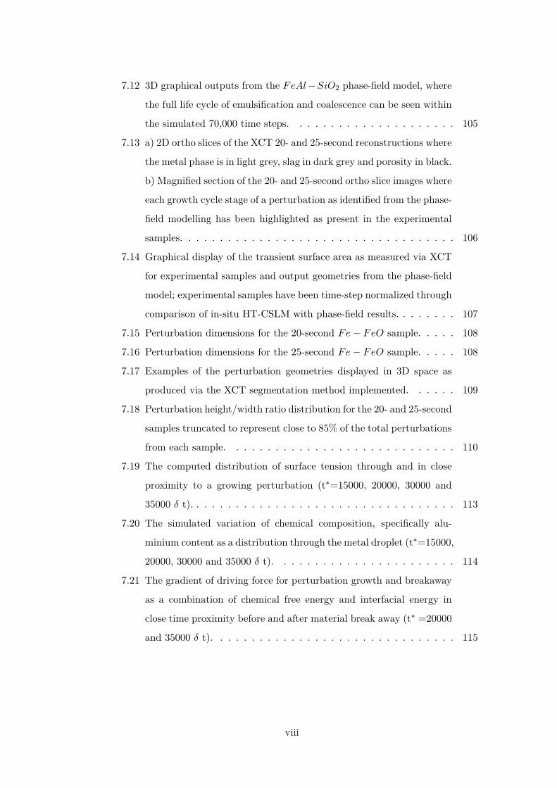
7.12 3D graphical outputs from the FeAl−SiO2 phase-field model, where

the full life cycle of emulsification and coalescence can be seen within

the simulated 70,000 time steps. . . . . . . . . . . . . . . . . . . . . 105

7.13 a) 2D ortho slices of the XCT 20- and 25-second reconstructions where

the metal phase is in light grey, slag in dark grey and porosity in black.

b) Magnified section of the 20- and 25-second ortho slice images where

each growth cycle stage of a perturbation as identified from the phase-

field modelling has been highlighted as present in the experimental

samples. . . . . . . . . . . . . . . . . . . . . . . . . . . . . . . . . . . 106

7.14 Graphical display of the transient surface area as measured via XCT

for experimental samples and output geometries from the phase-field

model; experimental samples have been time-step normalized through

comparison of in-situ HT-CSLM with phase-field results. . . . . . . . 107

7.15 Perturbation dimensions for the 20-second Fe− FeO sample. . . . . 108

7.16 Perturbation dimensions for the 25-second Fe− FeO sample. . . . . 108

7.17 Examples of the perturbation geometries displayed in 3D space as

produced via the XCT segmentation method implemented. . . . . . 109

7.18 Perturbation height/width ratio distribution for the 20- and 25-second

samples truncated to represent close to 85% of the total perturbations

from each sample. . . . . . . . . . . . . . . . . . . . . . . . . . . . . 110

7.19 The computed distribution of surface tension through and in close

proximity to a growing perturbation (t∗=15000, 20000, 30000 and

35000 δ t). . . . . . . . . . . . . . . . . . . . . . . . . . . . . . . . . . 113

7.20 The simulated variation of chemical composition, specifically alu-

minium content as a distribution through the metal droplet (t∗=15000,

20000, 30000 and 35000 δ t). . . . . . . . . . . . . . . . . . . . . . . 114

7.21 The gradient of driving force for perturbation growth and breakaway

as a combination of chemical free energy and interfacial energy in

close time proximity before and after material break away (t∗ =20000

and 35000 δ t). . . . . . . . . . . . . . . . . . . . . . . . . . . . . . . 115

viii

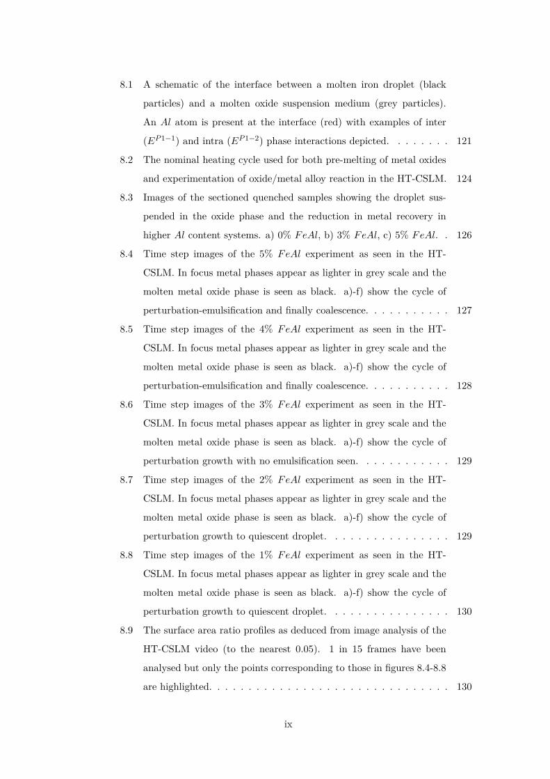
8.1 A schematic of the interface between a molten iron droplet (black

particles) and a molten oxide suspension medium (grey particles).

An Al atom is present at the interface (red) with examples of inter

(EP1−1) and intra (EP1−2) phase interactions depicted. . . . . . . . 121

8.2 The nominal heating cycle used for both pre-melting of metal oxides

and experimentation of oxide/metal alloy reaction in the HT-CSLM. 124

8.3 Images of the sectioned quenched samples showing the droplet sus-

pended in the oxide phase and the reduction in metal recovery in

higher Al content systems. a) 0% FeAl, b) 3% FeAl, c) 5% FeAl. . 126

8.4 Time step images of the 5% FeAl experiment as seen in the HT-

CSLM. In focus metal phases appear as lighter in grey scale and the

molten metal oxide phase is seen as black. a)-f) show the cycle of

perturbation-emulsification and finally coalescence. . . . . . . . . . . 127




perturbation-emulsification and finally coalescence. . . . . . . . . . . 128




perturbation growth with no emulsification seen. . . . . . . . . . . . 129




perturbation growth to quiescent droplet. . . . . . . . . . . . . . . . 129




perturbation growth to quiescent droplet. . . . . . . . . . . . . . . . 130

8.9 The surface area ratio profiles as deduced from image analysis of the

HT-CSLM video (to the nearest 0.05). 1 in 15 frames have been

analysed but only the points corresponding to those in figures 8.4-8.8

are highlighted. . . . . . . . . . . . . . . . . . . . . . . . . . . . . . . 130

ix

8.10 A schematic of the interface between an iron aluminium metal al-

loy (black particles represent iron atoms, red particles represent alu-

minium atoms) and a metal oxide medium (specifically silica molecules,

grey particles). An example of perturbation growth and necking is

given with varying diffusion distances of SiO2 bulk particles to per-

turbation head (SiO2−BAl−H , neck (SiO2−BAl−N ) and bulk droplet

(SiO2−BAl−D) qualitatively depicted. The strain angle θ as a result

of necking is also indicated. . . . . . . . . . . . . . . . . . . . . . . . 134

8.11 Global interfacial tension during the increase and reduction of inter-

facial area as measured for the 8% FeAl sample coupled with the free

energy gain of reaction to equilibrium for the 8, 5, 4, 3, 2, and 1%

FeAl systems. Period A is during initial light perturbation, B during

heavy perturbation, C fully emulsified, D ongoing coalescence and E

a fully coalesced droplet. . . . . . . . . . . . . . . . . . . . . . . . . . 137

A.1 An example of the sphere created from the minima averaging of per-

turbations . . . . . . . . . . . . . . . . . . . . . . . . . . . . . . . . . 156

A.2 a) A 2D slice of the 20-second sample, where the metal has been

highlighted in blue and all other material removed. b) The resul-

tant volume left after removal of the interior of the droplet through

overlapping of the minima averaging sphere. . . . . . . . . . . . . . . 157

A.3 The effective segmentation of the droplet surface as a result of the

automated method within the software splitting at defined minima.

Each colour represents a separately defined perturbation. . . . . . . 158

A.4 The grey-scale distribution of the sample space as defined from the

original average minima produced sphere size. The black circle is in

the space of the sphere and the grey values lighten radially outwards

from its surface. . . . . . . . . . . . . . . . . . . . . . . . . . . . . . . 158

x

List of Tables

4.1 IMPHOS heats and their starting “hot metal” compositions collected

by spark optical emission spectrometry. [4]. . . . . . . . . . . . . . . 37

4.2 The compositions of all metallic alloys used in HT-CSLM experiments

measured using ICP (where all N levels are <0.001%. . . . . . . . . 38

4.3 The compositions of all slags used in HT-CSLM experiments mea-

sured using XRF. . . . . . . . . . . . . . . . . . . . . . . . . . . . . . 38

5.1 Collation of previously reported residence times, with the experimen-

tal/modelling technique used. . . . . . . . . . . . . . . . . . . . . . . 44

5.2 Nominal start composition of hot metal used in IMPHOS trials. . . . 45

5.3 XCT scanning parameters used for the interrogation of solid emulsion

shards removed from the sampling pots. . . . . . . . . . . . . . . . . 51

5.4 Overall average and SD of %Tw, tr, and MCR for all blows. . . . . . 52

5.5 Initial results from XCT scanning of shard emulsion samples. The

number of discrete metal packages detected and their average diameter. 58

6.1 A summary of the previous findings of metal droplet size in oxygen

steelmaking emulsions. . . . . . . . . . . . . . . . . . . . . . . . . . . 70

6.2 XRF detected chemical composition of master slags, used in this study

and by Assis et al. . . . . . . . . . . . . . . . . . . . . . . . . . . . . 72

6.3 ICP detected chemical composition of Fe- alloys used in this study. . 73

6.4 Heating and quenching regime of all samples. ## being the period

of time a sample was held at high temperature for. . . . . . . . . . . 73

6.5 Parameters used within the two scanners. ∗ There is an additional

focusing step performed by an optic in the Zeiss machine, where x0.4

was used in this study. . . . . . . . . . . . . . . . . . . . . . . . . . . 75

xi

6.6 Summary of chemical analysis performed using the various techniques

described . . . . . . . . . . . . . . . . . . . . . . . . . . . . . . . . . 79

6.7 Raw data for surface area measurements of system 3. . . . . . . . . . 83

6.8 Raw data for volume measurements of system 2. . . . . . . . . . . . 83

7.1 Compositions of FeAl alloys used for the experiments in HT-CSLM

presented in mass %. Compositions were measured by ICP. . . . . . 111

8.1 Compositions of FeAl alloys used for the experiments in HT-CSLM

presented in mass %. Compositions were measured by ICP (all alloys

contained <0.001 %N). . . . . . . . . . . . . . . . . . . . . . . . . . . 122

8.2 Composition of the metal oxide mixture used for HT-CSLM exper-

imentation after pre-melting of reagent grade hand-mixed powders

presented in mass %. Compositions were measured by XRF. . . . . . 123

8.3 Literature values used for calculation of global interfacial tension and

dissipation of free energy as displayed in figure 8.11. . . . . . . . . . 136

xii

Acknowledgements

There are many people who have aided the pathway to completing this thesis, all of

whom I wish to express gratitude to. . . however I will keep it short.

To begin, I wish to thank Professor Sridhar Seetharaman. You created an environ-

ment to not only conduct exciting and interesting research, but also make friends,

develop myself and interact with the wider steel community. It has been a great

experience from the early days when I asked “when will there be more than two

people?” to the now spectacle of diversity there is within the group. I doubt many

see such change and progression during time as a student. The understanding and

trust you give to students creates a unique environment to challenge the experienced

and peruse the bold.

Deepest gratitude to:

Professor Mark Williams, Dr Jason Warnett, Dr Alireza Rahnama, Dr Zushu Li,

Dr Andre Assis, Dr Mohammed Tayeb, Dr Carl Slater, Dr Rohit Bhagat, Professor

Richard Fruehan, Dr Hongbin Yin colleagues, co-workers and Dr Alison Lusty.

- Your support, guidance, knowledge and time, has been inspiring and invaluable.

I would like to thank Tata Steel, and EPSRC for proposing and funding the project.

In addition I would like to thank:

Deborah Spooner (Mum), John Spooner (Dad), David McGovern and further family

and friends who both remain and have moved on.

- Your friendship, help and love have been a light of encouragement.

xiii

Victoria Lusty, I have not forgotten you, nor will I ever. Somehow you kept me

going, even when I was trying not to. With grace and humility you have driven me

to continue. My adoration and thanks are yours.

xiv

“The duty of youth is to challenge corruption” - Kurt Cobain

“Learning never exhausts the mind” - Leonardo da Vinci

xv

Declaration

This thesis is submitted to the University of Warwick in support of my application

for the degree of Doctor of Philosophy. It has been composed by myself and has

not been submitted in any previous application for any degree The work presented

(including data generated and data analysis) was carried out by the author except

in the cases outlined below:

• X-ray Computer Tomography scanning and image analysis was carried out by

Dr Jason Warnett

• Phase-field modelling was conducted by Dr Alireza Rahnama

• Chemical analysis of metal/slag droplet experiments was conducted by Dr

Andre Assis

Inclusion of Published Work

Parts of this thesis have been published by the author:

1. Spooner, S., Assis, A. N., Warnett, J., Fruehan, R. Williams, M. A. & Sridhar,

S., “CTSSC-EMI Symposium CSLM , XCT Couple Interrogation of the Emul-

sification Interaction between Free Steel Droplets Suspended in Steel Making

Slags”. EMMISYMP, Tokyo, (September, 2015).

2. Spooner, S., Warnett, J. M., Bhagat, R., Williams, M. A. & Sridhar, S.,

“Calculating the Macroscopic Dynamics of Gas/Metal/Slag Emulsion during

Steelmaking”. ISIJ Int. (2016). doi:10.2355/isijinternational.ISIJINT-2016-

361

3. Spooner, S., Assis, A. N., Warnett, J., Fruehan, R. Williams, M. A. & Sridhar,

S.,“Investigation into the Cause of Spontaneous Emulsification of a Free Steel

xvi

Droplet; Validation of the Chemical Exchange Pathway”. Metall. Mater.

Trans. B (2016). doi:10.1007/s11663-016-0700-3

4. Tayeb, M. A., Spooner, S., & Sridhar, S., “Phosphorus: the noose of sustain-

ability and renewability in steelmaking”. JOM, 66 (9) (2014), 1565-1571

5. Assis, A. N., Warnett, J. M., Spooner, S., Williams, M. A., & Sridhar, S.,

“Spontaneous Emulsification of a Metal Drop Immersed in Slag Due to De-

phosphorization: Surface Area Quantification”. Metall. Mater. Trans. B

568-576 (2014). doi:10.1007/s11663-014-0248-z

6. Under Submission - Spooner, S., Rahnama, A., Warnett, J. M., Williams, M.

A., & Sridhar, S., “Spontaneous Emulsification during Material Exchange in

Two Phase Liquid Systems”. Sci. Rep. (Submitted January 2017)

7. Under Submission - Spooner, S., Li, Z., & Sridhar, S., “Spontaneous Emulsi-

fication as a Function of Material Exchange”. Sci. Rep. (Submitted January

2017)

During the period of study this thesis was produced, further findings were also

published:

1. Slater, C., Spooner, S., Davis, C. & Sridhar, S. “Observation of the reversible

stabilisation of liquid phase iron during nitriding”. Mater. Lett. 173, 98-101

(2016).

2. Slater, C., Spooner, S., Davis, C. & Sridhar, S. “Chemically Induced Solidifi-

cation: A New Way to Produce Thin Solid-Near-Net Shapes”. Metall. Mater.

Trans. B: Process Metall. Mater. Process. Sci. 47, 1-4 (2016).

3. Rahnama, A., Spooner, S. & Sridhar, S. “Control of intermetallic nano-particles

through annealing in duplex low density steel”. Mater. Lett. 189, 13-16 (2017).

xvii

Abstract

The steel industry is facing significant competition on a global scale due to the drive

for light-weighting and cheaper more sustainable construction. Not aided by over-

supply in geographic sectors of the industry, there is significant competition within

the slowly shrinking sector. The recent growth in developing countries through

installation of modern plant technology has led to the reduction in unique selling

points for mature steelmaking locations. As such, to compete with the equalling

product capability and innate cheaper production costs within developing areas the

industries in Europe and North America require significant improvements in produc-

tivity and agile resource management. To date the basic oxygen furnace has been

somewhat treated as a black box within industry, where only control parameters are

monitored, not the fundamental mechanisms within the converter. Studies over the

past 30 years have shown the basic oxygen furnace is unable to attain the thermo-

dynamic minimum phosphorus content within the output liquid steel. Coupled with

the need to drive down resource cost, with a potential for high content phosphorus

ores the internal dynamic system of the basic oxygen furnace requires more rigorous

understanding.

With the aid of in-situ sampling of a pilot scale basic oxygen furnace, and

laboratory studies of individual metal droplets suspended in a slag medium (known

to be a key driving environment for impurity removal) the present project aims

to provide insight into the transient interfacial area between slag and liquid metal

through basic oxygen steelmaking processing. Initially the macroscopic dynamics

including the amount of metal suspended in the gas/slag/metal emulsion, the period

of time it is suspended for, and the speed at which it moves, is investigated. It was

found that these parameters vary greatly through the blow, with a normal peak in

residence times near the beginning of the blow and a dramatic increase in metal

circulation rates at the end of the blow, when foaming is reduced or collapsed.

Further to this, a method of interrogating the size of metal droplets within the slag

layer using X-ray computed tomography is introduced.

The study then progresses into the microscopic environments that individual

droplets are subjected to during steel processing. Initially the cause of sponta-

neous emulsification in basic oxygen furnace type slags is investigated through high

temperature-confocal scanning laser microscopy/X-ray computed tomography led

experimentation, with the addition of null experiments conducted to rationalize the

experimental technique. It was found that the flux of oxygen across the interface

was the cause and thus the confirmation of material transfer across the interface

being the driving force. Furthermore the physical pathway of emulsification is inter-

rogated and quantified, with in-situ observation of spontaneous emulsification in the

high temperature-confocal scanning laser microscope enabled through use of opti-

cally transparent slags. The life cycle of perturbation growth, necking and budding

is observed and quantified through high-resolution X-ray computed tomography. In

addition a phase-field model is developed to interrogate slag/metal systems in 2D

and 3D variations, giving rise to the ability to track the cause of emulsification and

to predict its occurrence.

Finally the project progresses with the in-situ investigation of spontaneous

emulsification as a function of initial metal composition. The behaviour of droplet

spontaneous emulsification is seen to reduce in severity and subsequently to decline

into a non-emulsifying regime below a critical level. Free energy calculations coupled

with a measure of the global interfacial tension increase give quantifiable reasoning

as to the behaviour seen.

ii

List of Abbreviations

%Tw Percentage Tap Weight

BF Blast Furnace

BOF Basic Oxygen Furnace

BOS Basic Oxygen Steelmaking

CFD Computational Fluid Dynamics

DRI Direct Reduced Iron

EAF Electric Arc Furnace

HT-CSLM High-Temperature Confocal Scanning Laser Microscopy

ICP-MS Inductivly Coupled-Mass Spectroscopy

IMPHOS Improved Phosphorus Refining

LA-ICPMS Laser-Ablation Inductivly Coupled-Mass Spectroscopy

LD Linz Donawitz

LD-LBE LD-Lance Bubbling Equilibrium

LD-NRP LD-Converter Type Dephosphorization Process

LD-ORP LD-Converter Optimized Process

MURC Multi Refining Converter Process

NRP Ladle-type Dephosphorization Process

OHF Open Hearth Furnace

i

RRS Rosin-Rammler-Sperling

SE Spontaneous Emulsification

SEM Scanning Electron Microscope

SIMS Secondary Ion Mass Spectroscopy

USA United States of America

WDS Wavelength Dispersive Spectroscopy

XCT X-ray Computed Tomography

ZSP Zero Slag Process

ii

Chapter 1

Introduction

1.3 billion tons of steel were produced in 2015 across 65 countries [1] making it the

largest industrially produced material in the world by weight. This along with overall

significant growth of 30% since 2006 gives reason for the global need of the steel

industry to adapt and survive. There are two main routes of production today: the

Electric Arc Furnace (EAF) and the integrated Blast Furnace-Basic Oxygen Furnace

(BF-BOF) route. Combined they account for 99% of steel production worldwide

(30% and 69% respectively) with the remaining 1% through production via Open

Hearth Furnace (OHF) and other processes [2]. The relative proportions differ widely

from country to country with for example North America producing 60% of its steel

through the EAF whereas Europe is heavily dependent on the BF-BOF route at 70%

of total production. Scrap and hot metal are charged into the BOF whereas the EAF

is mainly charged with scrap and pig iron; however recent and continued reduction in

natural gas prices following successful shale rock exploration has encouraged the use

of direct reduced iron (DRI) in North America and other countries rich in natural

gas such as those in the Middle East [2].

DRI can be used to substitute scrap and pig iron, for both economic and

compositional control reasons. With the extensive markets of China and India there

is a huge overcapacity of production in local areas with the ability to undersell on

the global stage. Figure 1.1 shows the global production of steel in each region

of the world for 2013. As a result developed markets are searching for ways to

stay competitive and justifiable in years to come. One way this is being explored

is through diverse and untraditional approaches to steel production, for example

end-point variable product control.

1

0

200

400

600

800

1000

1200

EuropeanUnion

OtherEurope

CIS NAFTA Centraland SouthAmerica

Africa MiddleEast

Asia China

Mil

lio

n T

on

s

Figure 1.1: Global production statistics (2013) with relation to tonnage. [2]

With the price of iron ore exponentially growing in present years, the need

for resource flexibility is integral to a sustainable primary steel industry. Sources of

iron ore quality have great variability in levels of iron content, as well as impurity

levels. Phosphorus is used as an example in figure 1.2, where cheaper ores from Peru

and China for instance have much higher initial phosphorus content.

0

0.02

0.04

0.06

0.08

0.1

0.12

0.14

0.16

USA Brazil Peru Russia China

Ph

osp

ho

rus

wt%

Figure 1.2: Phosphorus impurity levels in ore sources around the globe.

Predefined treatments for sulfur and optimised carbon removal process in

the BOF leave phosphorus as a chemical restriction on usable ore within European

plants. The BOF is relied upon for phosphorus removal; with the introduction of lime

based slags providing a partitioning phase for refined phosphorus to be held. This

process is however primarily operated and optimized for carbon removal from steel

which has been heavily enriched during coke reduction in the BF [3]. As previously

2

mentioned EAF’s are primarily charged with scrap, however with the addition of

DRI phosphorus content can again become an issue for steel product via this route.

Considering this the pathway and fundamental reaction kinetics of phospho-

rus removal is to be investigated under pseudo-industrial conditions. Data from the

European Commission funded project “IMPHOS: Improved phosphorus refining” [4]

in conjunction with lab-based emulsification experiments will be used to gain greater

understanding into the fundamental conditions responsible for phosphorus removal.

The aim of the project is to provide insight into factors which could be manipulated

to increase overall BOF performance.

Currently P removal is through the partition between liquid metal and slur-

ries of metal oxides (slag). This has been the provided pathway in steelmaking

for many years. Studies of the last 30 years however have consistently reported

the thermodynamic maximum partitioning of phosphorus is not attained through

conventional BOF operation; thus current processes are kinetically hindered. Devel-

opments of further technologies such as torpedo ladle refining, double slagging and

double converter refining have been explored and subsequently implemented in some

countries (Japan, Korea and China mostly). These systems are working to combat

higher purity demands of the consumer, for instance interstitial-free high strength

pipeline steels. Although these systems are in place, they are for the most part

incredibly inefficient, causing temperature loss from the hot metal and productivity

reduction. The necessity for increase of workforce, large amount of excess waste and

loss of material through ladle refining are further issues. For a sustainable industry

more effective ways of combating phosphorus levels is desperately needed.

1.1 Objectives of Study

The overall objective of this project is to offer quantification to the transient in-

terfacial area between liquid metal and metal oxide phases in the BOF. This is in

order to provide insights into factors of influence for long term steel production and

dynamic product design.

The study can be broken down into an investigation into the macroscopic

dynamics within the BOF through use of IMPHOS data, giving improved knowledge

of the quantity of metal, how long it is suspended and the circulation rates within

3

the gas/slag/metal emulsion in the BOF. These findings will inform future models

as to the potential of refining through quantification of interfacial area, as well as

the turnover of reactive phases in contact with each other, and hence the level of

sustained chemical potential while the interface is present.

Further to this the effects of refining on individual droplet dynamics will be

investigated through the coupling of High-Temperature Confocal Scanning Laser

Microscopy (HT-CSLM), X-ray Computed Tomography (XCT) and the further ad-

dition of phase-field modelling for predicting interfacial phenomena. Efforts will be

made to define the cause, level of influence required and the pathway by which spon-

taneous emulsification occurs, in order to offer quantification as to the interfacial

area development, as well as knowledge on how the phenomenon may be encouraged

or prevented depending on the application. This study will be significantly relevant

to slag/metal reaction in a broader scheme of steelmaking, such as those seen in la-

dles during secondary steelmaking, the tundish before casting, electro-slag refining,

interaction with mould powders during casting and droplets generated in the HIs-

arna process. The physical pathway and ability to model spontaneous emulsification

presents knowledge applicable further afield, such as to copper production, silicon

nano-particle synthesis or waste recovery.

1.2 Thesis Structure

Following from this brief 1. “Introduction” the layout of the first half of this thesis

follows an ordered path of: 2. “Underpinning knowledge”; in this section the basic

background on steelmaking is presented, along with deeper discussion on the BOF,

phosphorus reactions, droplet generation in the BOF, droplet residence times in the

BOF and spontaneous emulsification previously witnessed in slag/metal reaction

systems. 3. “Formulating the Research Approach”; where hypotheses are identified

and the approach to interrogate them is discussed. 4. “Experimental Methods”;

where the overarching techniques used within the study are introduced and briefly

described (more in-depth comments on the experimental methods are given in the

relevant results chapters).

Following on from these background chapters, the thesis contains four results

chapters: 5. “Calculating the Macroscopic Dynamics of the Gas/Metal/Slag Emul-

4

sion During Steelmaking” where the transient environment of metal droplets in the

BOF emulsion phase is interrogated; 6. “Investigation into the Cause of Sponta-

neous Emulsification of a Free Steel Droplet; Validation of the Chemical Exchange

Pathway” which includes standardization of experimental techniques against those

previously reported in the literature as well as rationalization as to why spontaneous

emulsification occurs in the presented systems; 7. “Quantifying the Pathway and

Predicting Spontaneous Emulsification During Material Exchange in a Two Phase

Liquid System”, in this chapter the physical morphology of the perturbed droplet

surface is examined along with the introduction of a phase-field model to offer the

ability to predict spontaneous emulsification. 8. “Spontaneous Emulsification as

a Function of Material Exchange”, finally the implication of material exchange on

interfacial tension is discussed along with the interrogation of the phenomenon using

the developed in-situ observation technique to study the level of material exchange

required for emulsification to occur, this is rationalized through dissipation of free

energy calculations.

Finally the experimental and modelling results are brought together in an

encompassing “Conclusions and Suggested Further Work” section, where comments

on the relevance and possible impact of findings to industrial practice are made along

with suggestions of future work to guide the development and greater understanding

of the findings and implications presented.

5

Chapter 2

Underpinning Knowledge

2.1 Modern History of the Steel Industry

Steel is an iron matrix alloy usually containing less than 1% carbon. It is used most

frequently in the automotive, construction, pipes, and consumer goods sectors. Steel

is produced in many shapes and forms including bars, sheets, wire, rod or pipe as

needed by the intended consumer.

The process of steelmaking has undergone many changes in the last century

based on the political, social and technological environment. In the 1950s and 60s,

demand for high quality steel encouraged the industry to produce large quantities

via integrated steel mills. Large integrated mills were thrust into the driving seat

of the industry throughout the USA and Europe, with the ability to produce large

quantities of consistent steel products from raw materials [2]. However these plants

required high capital costs and were constructed with limited flexibility.

The 1970s saw thermal efficiency made a priority within steel production.

Integrated plants contain an innate efficiency due to economies of scale and factors

such as heat retention when dealing with large volume. Despite this, improvements

in common production practices became vital to viability. Previously (1950s and 60s)

steel production had been dominated via batch processes, as a result idle equipment

was not uncommon as an individual batch was taken through each process stage from

raw materials to finished product. Huge energy savings were made by the large scale

uptake of processes such as continuous casting and the continuously supply of raw

materials to the blast furnace.

As environmental concerns gained importance in the 1980s and 90s, regu-

6

lations became more stringent again changing the steelmaking industry. By 1995,

compliance with environmental legislation was estimated to make up 20-30% of the

capital costs [5] for new steel production. Competition has also increased during the

recent decades due to decreasing markets and increasing international steel capacity.

The nature of alternative material use and global over-supply has driven reduction

in production cost and an increase in product quality.

Global economics and legislation is driving a change to just-in-time tech-

nology through the mass uptake of mini-mill technology in the USA and other

geographic sectors as opposed to the previously dominating status of integrated

production. Mini-mills rely on steel scrap as a base material rather than ore. It

is expected mini-mills will never completely replace integrated steel plants as they

cannot maintain the tight control over chemical composition and thus cannot con-

sistently produce high quality steel. Mini-mills work through a narrow production

line and cannot produce the speciality products integrated plants currently provide.

Technology however continues to improve and since the mid-1990s the introduction

of direct reduced iron and pig iron sources to the scrap production route has allowed

for access to a greater diversity of products [6].

2.2 The Integrated Steel Plant

Steel production through an integrated steel plant involves three primary product

steps. First, the heat source used to melt iron ore is produced; followed by the

melting and reduction of iron ore in the blast furnace; finally the molten metal is

reacted with oxygen to form the low carbon compositions of steel. The steps can be

conducted at one facility through an on-site power station and collocation of BF and

BOS facilities. However power is often supplied from off-site producers. A schematic

of a modern integrated mill is shown in figure 2.1.

2.2.1 Coke Making

Coke is the solid carbon fuel used to melt and reduce iron ore. Coke production

begins with pulverised bituminous coal. The coal is fed into a coke oven, sealed and

heated to around 1573 K for 14 to 36 hours. Coke is produced in a batch process,

with multiple ovens operating simultaneously to offer a constant supply of material

7

Crude Steel

Figure 2.1: A schematic of the modern integrated steel mill [7].

to the BF.

Heat is frequently transferred from one oven to another, reducing energy re-

quirements [8]. After the coking process is finished, the coke is moved to a quenching

tower where it is cooled with water spray. Once cooled the coke is moved directly

to an iron making furnace or into storage.

2.2.2 Ironmaking

During ironmaking, iron ore, coke, heated air and limestone or other fluxes are fed

into the BF. The heated air causes the coke to combust, which provides heat and

the carbon source for iron production. Limestone or variants (e.g. dolomite) are

added to react with and remove the acidic impurities from the molten iron. The

limestone-impurity mixture floats on the top of the liquid metal forming a slag and

can be skimmed off during the continuous process.

8

Sintering products may also be added to the furnace. Sintering is the process

in which solid wastes are combined into a porous mass which can be added to the

BF. The wastes can include iron ore fines, pollution control dust, coke breeze, water

treatment sludge and flux. Sintering plants help reduce solid waste by combusting

waste products and capturing trace levels of iron present in the mixtures. Sintering

plants are not used at all steel production sites [6] [9]. The process of iron making

has issues of phosphorus carry over from the originating ore as well as coke additions.

2.2.3 Basic Oxygen Steelmaking

Molten iron from the BF is sent to the BOF. The BOF gives utility for the final

refinement of the iron into steel. High purity oxygen is blown into the furnace

via a top lance at supersonic speeds. The oxygen combusts with elements such

as carbon and silicon in the molten iron. Further fluxes are fed into the BOF to

offer a partitioning oxide phase for the removal of impurities such as phosphorus,

manganese and titanium etc. Further to refining in the BOF, liquid steel often

undergoes alloying steps within the ladle to deliver the required compositions.

The resulting steel is most often cast into slabs, beams or billets. Further

shaping of the metal may be conducted within steel foundries, which re-melt the

steel and pour the liquid into moulds, or at rolling facilities with both hot and cold

conditions, depending on the desired product shape and properties.

Slag is a significant by-product of the BOF. Slag is essentially a slurry of

metal oxides in liquid state. The most common components within slag of the steel

industry are CaO, FeO (in variable oxidation states), Al2O3, SiO2, MgO, Cr2O3,

TiO2, P2O5 and MnO. The ratio of these oxides affects the melting point, viscosity,

and impurity partitioning capability along with other processing factors such as foam

stability and refractory wear. Of the varying properties the slags basicity is often

considered one of the more important features; the basicity is effectively a measure of

free oxygen, meaning network forming oxides such as SiO2 reduce basicity whereas

network breaking oxides such as CaO increase basicity. The two selected examples

are in fact the most influential and are thus combined to calculate the binary basicity

(%CaO/%SiO2), the quickest and most common way to understand how a slag is

likely to behave during a process or reaction. With the likely high levels of FeO

within the recovered BOF slag, there is significant potential for internal recycling

9

as an additive in the sintering process [10]. However due to its relatively low iron

content compared to raw materials, recently there has been significant activity in

its use as carbon sinks, road materials and water purification systems [11].

Hot gases are a further by-product of the BOF, with modern furnaces being

equipped with air pollution control equipment able to contain and cool the gases.

The gas is quenched and cooled using water and cleaned of suspended metals and

other solids. The process produces air pollution control dust [10] and water treat-

ment plant sludge [12].

Steel Production from Scrap

Steelmaking from scrap involves melting of scrap, removing impurities and casting

into a desired shape. The EAF is often used, and melts with the use of electrical

energy in the presence of oxygen. The process is a direct method to produce desired

products (as opposed to the multiple steps required through the BF-BOF route)

offering the potential to be economically viable on a much smaller scale. Frequently

mills producing steel with EAF technology are referred to as mini-mills. In addition

it is possible to utilise a portion of scrap within the BOF. The key reasons for doing

so are temperature control and the fluctuation in raw material price on a global

scale; whereas scrap prices are often dictated within smaller geographic regions due

to oversupply and government preference through legislation for internal recycling.

2.2.4 Steel Forming and Finishing

After molten steel is released from either the BOF or EAF, it must be formed into

its final shape and finished to prevent corrosion. Traditionally steel was poured into

a conventional ingot and stored until a specific final product was required. However

current practices favour continuous casting where the steel is poured directly into

semi-finished shapes. Continuous casting saves time by: reducing the steps required

to produce the desired shape; it increases length versatility of product; and lends

itself well to the modern just-in-time manufacturing approach to production and

acquisition.

After cooling within the mould further shaping is conducted through hot or

cold forming. Hot forming consists of heated steel being passed between rollers until

it reaches its desired thickness. The process lends itself to the production of slabs,

10

strips, bars or plates from the steel.

Cold forming is used to produce wire, tube, sheet and strip. This process

involves the steel being passed between rollers without being heated to reduce thick-

ness. The steel is then heated in an annealing furnace to improve the ductile prop-

erties. Cold rolling is more time consuming, but is used because products taking

this route have better mechanical properties, better machinability and can more

easily be manipulated into challenging sizes and thinner gauges [8]. After rolling is

completed the steel pieces are finished to prevent corrosion and improve properties

of the metal [8] [13]).

2.3 The Basic Oxygen Furnace

As previously discussed the BOF serves as a refining vessel for hot metal produced

in the BF. With the incorporation of a desulfurization pre-treatment before entering

the BOF, the primary functions remaining are decarburization, dephosphorization

and temperature adjustment [8].

Carbon content is around 4 wt% when hot metal enters the BOF, the majority

of which is present due to the reducing process in the BF being conducted through

addition of coke. With regards to phosphorus, the sources are from iron ore, coke

during ironmaking and poor quality scrap input at the BOF stage. Under the

reducing conditions within the BF all phosphorus entering the BF is carried over

into the output hot metal.

The dephosphorization reaction is facilitated in several ways through oxygen

steelmaking. Firstly the introduction of desulfurization pre-treatments reduces the

competition for interfacial sites between liquid steel and slag, allowing phosphorus

removal to begin at a high rate from early in the blow. With controlled oxygen

partial pressure and lime introduction, the chemical pathway for dephosphorization

is enabled through the oxidation of Fe to FeO and availability of Ca for inorganic

complex formation [14] [15] such as in equation 2.1:

2CaO + 2PO2.5 = 2CaO.P2O5 (2.1)

With a target liquid slag composition which maximizes the P partition at

high binary basicity’s (CaO/SiO2) of 3-5, which varies as a result of incomplete lime

11

dissolution and the extension of blow time past that needed for sufficient carbon

removal (end blow period), the BOF presents a period of favourable environment

with reduced competition for the dephosphorization reaction.

Problems with the existing practice are caused inherently by additional func-

tion requirements. Including: the removal of carbon; a competing reaction for avail-

able oxygen [16] (see equations 2.2 2.3); unfavourable high target temperature re-

quired for the material to stay liquid in transport to the casting operation [17]; and

the converter size/batch mass which inhibits the controllability of micro conditions

and predictive interface formation [18] [19].

[C] + (O2)→ (CO2) (2.2)

(CO2) + [C]→ 2(CO) (2.3)

where material within () is in a gas phase and those within [] are in the liquid

steel.

Within the BOF, there are several locations/zones where refining takes place.

Initially the quiescent interface of the bulk bath-slag, being the simplest region, is

now thought to be less significant in controlling phosphorus refining. Secondly the

“hot zone” (the location where the steel bath surface is directly struck by the im-

pinging oxygen jet) as a kinetically released hyper-reaction site due to high compar-

ative temperatures and abundance of oxygen [20] [21] [22]. Finally the three phase

gas/slag/metal emulsion presents a possibility of significant influence over the gov-

erning phosphorus removal rate due to the drastically larger interfacial area provided

through the dispersion of metal droplets (in comparison to the quiescent interface).

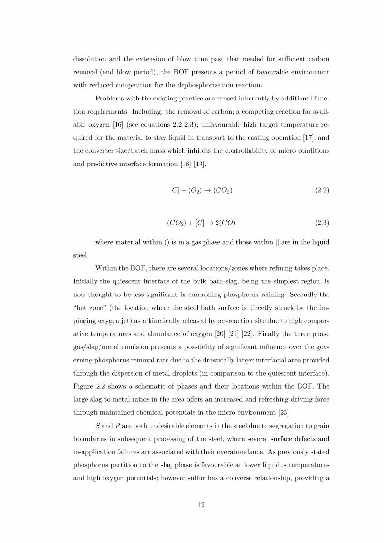
Figure 2.2 shows a schematic of phases and their locations within the BOF. The

large slag to metal ratios in the area offers an increased and refreshing driving force

through maintained chemical potentials in the micro environment [23].

S and P are both undesirable elements in the steel due to segregation to grain

boundaries in subsequent processing of the steel, where several surface defects and

in-application failures are associated with their overabundance. As previously stated

phosphorus partition to the slag phase is favourable at lower liquidus temperatures

and high oxygen potentials; however sulfur has a converse relationship, providing a

12

“Hot Zone”

Figure 2.2: Schematic of the BOF, whith key phases/locations labled [24].

difficult if not near impossible situation to control both residual elements levels at

the same time [2] [6] [25] [26] [27] [4].

2.3.1 Further Dephosphorization Technologies

Advanced converter-type hot metal pre-treatments for dephosphorization have been

developed and are in use commonly in markets such as Japan and Korea to address

the need for ultra-low P level in steel production. Since initial introduction in 1993,

several technologies have been implemented.

An initial example is the Zero Slag Process (ZSP), based on desiliconization

to below 0.1 wt% Si prior to dephosphorization. Each is conducted within a separate

ladle station between BF output and prior to BOF loading. Via such a method there

is claim that slag volume may be markedly reduced and iron yield increased [13].

Two methods implemented within de-P stations are the ladle-type dephos-

13

phorization process (NRP) and the LD-Converter-Type-Dephosphorization process

(LD-NRP). In each process calcium requirement is much less as low silicon levels

are present; CaO.P2O5 may form in preference to CaO.SiO2 at low temperatures

favourable for efficient de-P . The LD converters perform decarburization followed

by dephosphorization. The average phosphorus content after such treatment is less

than 0.012 wt%. Although these processes are considerably innovative, the capital

cost in addition to the increase in processing times are major constraints of the

processes which inhibit international acceptance and application.

LD converter optimized process (LD-ORP) is an example of technology which

uses two double converter operations. This breaks down into desiliconization and

dephosphorization coupled removal in one converter followed by decarburization in

a second vessel. In multi refining converter processes (MURC) the hot metal is de-

phosphorized and decarburized sequentially in the same converter separated through

de-slagging (slag discharging by tilting the converter) [13]. The advantages of such

a process over conventional hot metal pre-treatment in a torpedo ladle or molten

metal ladles is the improved productivity through high oxygen potentials (due to di-

rect high speed oxygen blowing), low slag basicities (dropping the slag volume) and

the low temperatures all favourable to dephosphorization. The MURC process does

not require a pre-desiliconization step or a change in vessel; while offering the ability

to reuse the rich carbon treatment slag (high in FeO) for dephosphorization in the

following charge. Such considerations promote the use of MURC processing over

LD-ORP. The introduction of slag replacement systems such as the MURC process,

notwithstanding its advantages, causes a relatively large increase in requirements

of lime provision, flux and other slag components; as such there is a greater waste

output [2] [13].

2.4 Phosphorus reaction: Thermodynamics and Kinet-

ics

The thermodynamics and kinetics of phosphorus reactions are important aspects

to consider towards understanding of phosphorus behaviour in the steelmaking pro-

cesses.

Steelmaking oxygen partial pressures favour the stability of phosphorus in

14

the slags as phosphate ions (PO3−4 ) [28]. As such, the phosphorus oxidation follows

the following ionic reaction:

P + 2.5(FeO) + 1.5(O2−) = (PO3−4 ) + 2.5Fe (2.4)

The equilibrium constant of equation 2.4 can be defined as [29]:

K =aPO3−

4

aP a5/2FeO a

3/2O2−

= C(%P )γPO3−

4

[%P ](T.Fe)5/2γ5/2FeOa

3/2O2−

(2.5)

The phosphorus partition ratio has long been used as a criterion to evaluate

the slag’s capability to remove phosphorus from the melt; it is usually defined as:

LP = (%P )[%P ] (2.6)

Researchers have interchangeably expressed the capacity of a slag to contain

phosphorus by apparent phosphorus partition, defined in equation 2.7

LP = (LP )(T.Fe)5/2

(2.7)

The logarithmic of apparent phosphorus partition has been expressed as a

function of slag composition, and temperature using multiple regression analysis of

controlled equilibrium experimental data, for example [29] [30]:

log( LPFe2.5

t

) = 0.06[(%CaO) + 0.37(%MgO) + 4.65(%P2O5)− 0.05(%Al2O3)

− 0.2(%SiO2)] + 11570T− 10.52 (2.8)

In the above equations: The underlined/square brackets represent the content

in the metal, while the parentheses denote the content in the slag

ai : Activity of component i in the metal or slag

γi : Activity coefficient of componenti

T.Fe : Total iron in the slag

C : Term, which includes the conversion factors

At low concentrations of phosphorus, and oxygen, as in most of the exper-

imental melts, the phosphorus activity coefficient is close to unity; therefore mass

15

concentrations have been used in formulating the equilibrium constant in the above

reaction. From the exothermic phosphorus reaction; the reaction is proceeding to

the right, and would achieve relatively high phosphorus partition when satisfying

conditions including; high amounts of lime (CaO) in the slag (oxygen anions), high

oxygen content in the slag (FeO activity) and low activity of phosphate ions. Ac-

cordingly, high lime, and comparative lower temperatures are favourable for the

dephosphorization reaction.

Phosphorus partition in the BOF is not at predicted equilibrium for the

conditions, and intrinsically kinetics must be considered [22]. This non-equilibrium is

primarily caused by the kinetic conditions in the steelmaking operation where fluxes,

oxygen, and carbon addition take place continuously or in batches at different stages

of the melt-process, semi-continuous slag flushing, and the resultant temperature

changes [31] [15] [32].

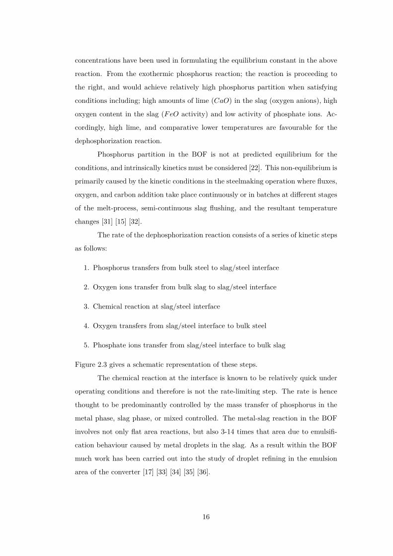
The rate of the dephosphorization reaction consists of a series of kinetic steps

as follows:

1. Phosphorus transfers from bulk steel to slag/steel interface

2. Oxygen ions transfer from bulk slag to slag/steel interface

3. Chemical reaction at slag/steel interface

4. Oxygen transfers from slag/steel interface to bulk steel

5. Phosphate ions transfer from slag/steel interface to bulk slag

Figure 2.3 gives a schematic representation of these steps.

The chemical reaction at the interface is known to be relatively quick under

operating conditions and therefore is not the rate-limiting step. The rate is hence

thought to be predominantly controlled by the mass transfer of phosphorus in the

metal phase, slag phase, or mixed controlled. The metal-slag reaction in the BOF

involves not only flat area reactions, but also 3-14 times that area due to emulsifi-

cation behaviour caused by metal droplets in the slag. As a result within the BOF

much work has been carried out into the study of droplet refining in the emulsion

area of the converter [17] [33] [34] [35] [36].

16

Liquid Metal Liquid Slag

P O2-

3. Reaction

1. 2.

4. 5.O PO4

3-

Figure 2.3: The kinetic steps required for phosphorus removal from liquid steel.

2.5 The Interfacial Area of reaction within the Emul-

sion

2.5.1 Droplet Size Distribution

The metal phase within the BOF slag/gas/metal emulsion has been quantitatively

investigated by only a few researchers on an industrial or laboratory scale. These

investigations have focused primarily on identifying the size distribution of the metal

droplets, weight percentage and surface area at various stages of blow or under

controlled laboratory conditions.

The investigation by Meyer [37] of metal droplet size distribution was con-

ducted using a 230 ton BOS converter. Material which was ejected through the

converter tap hole was rapidly cooled on large steel pans positioned outside the

vessel. The size distribution was then measured using sieving technology after the

emulsion material had undergone crushing, screening and magnetic profiles to sep-

arate the metal phase from the slag material. Droplet size ranged between 14-100

mesh and the emulsion was reported to contain up to 80% metal material by weight

at a particular blow period; however some of the droplets exhibited features such

as cavities caused by CO nucleation within the droplets. Skewing of droplet size

distribution towards finer sizes is also discussed due to fracturing of larger droplets

during the physical breakup procedures.

17

A further study conducted by Cicutti et al [23] focused on slag-metal reac-

tions in an LD-LBE converter. Samples of the gas/slag/metal emulsion were col-

lected simultaneously from a 200 ton converter during full operation using a uniquely

designed lance; the lance allowed for sampling during process and at different times

of the blow. From the separation and post analysis of the metal fraction within the

collected emulsion samples it was found droplet sizes ranged from 230 - 335 µm. In

addition to this the droplet size distribution agrees well with the Rosin-Rammler-

Sperling (RRS) function, given in equation 2.9:

R = 100exp[−( dd′

)n]% (2.9)

where R is the cumulative weight of droplets retained in the sieve (%), d is

the upper limit of class diameter in a given class (µm), d’ is the size parameter -

mean particle size (dimensionless) and n the distribution parameter - measure of

spread of particle sizes (dimensionless).

As with Meyer [37], Cicutti [23] reported droplets being more decarburized

than the metal within the bulk bath at a given time. Further to this droplets of

smaller sizes had progressed further through decarburization than large droplets, and

overall the direct decarburization of metal droplets within the emulsion was proposed

as a significant factor contributing to the global decarburization performance with

the BOF.

Millman et al [4] investigated the processing events with a 6 ton BOF pilot

plant converter with specific emphasis on the phosphorus behaviour during the blow.

Samples of the emulsion, slag and bulk metal bath were simultaneously collected at

2 minute intervals during an average blow time of 16 minutes. Emulsion samples for

two heats were microscopically analysed to produce size distributions of the emulsion

metal droplets and voids. Independent of blow time and measured across a limited

size range of 0 - 400 µm, the majority of droplets possessed a diameter below 100

µm. In addition CFD modelling was employed to simulated droplet generation and

the reported findings from both modelling and experimental avenues had signifi-

cant correlation for the lower emulsion levels, while the model over-predicted size

distribution at higher levels within the converter.

Price [38] conducted studies on the significance of the emulsion in carbon

removal through sampling an industrial working BOF using an ‘in-blow bomb’ ca-

18

pable of collecting slag and emulsion samples simultaneously. The predominant size

range of droplets within the emulsion was found to be 100 - 2000 µm; although it

was noted that agglomeration of droplets on the sampler support chain may have

affected the credibility of reported droplet size distributions.

Block [39] and Urqhuart [40] collected samples from inside the reaction area

with the former using a specially designed lance to sample the emulsion phase.

Tokovoi [41] sampled the slag/metal emulsion by collecting droplets from the upper

layer. Resch [42] and Baptizmanskii et al [43] also sampled the emulsion; Resch

[42]) by tilting the reaction vessel and Baptoizmanskii [43] by cutting a hole in the

crucible.

Lange and Koria [44] sampled oxidised drops by using a combination of

high speed filming (viewing the impingement area of the oxygen jet) and collecting

splashed emulsion samples from the top of a converter. Smaller droplets were spher-

ical whereas larger droplets (those <2000 µm) appeared to have flattened. Droplet

size distribution was again found to obey the RRS distribution function. Droplet

size ranged between 500 and 5000 µm diameter mostly, however larger droplets up

to 70,000 µm were also found. The conclusions drawn were larger droplets (those

<2000 µm) decarburized less because of their inherent smaller surface area to volume

ratio and lower emulsion residence time.

Koria and Lange [45] further experimentally investigated the disintegration

of 5% FeC droplets falling vertically through a high-velocity jet. Results showed

that after fragmentation by the high-velocity jet into secondary droplets, further

breakup does not occur; a finding which led the authors to conclude droplet size

distribution is solely a characteristic of the Weber number. In further studies the

authors discuss the insignificance of initial droplet diameter on the final droplet size

distribution [46].

Nordquist et al [47] conducted metal droplet size distribution experiments

within a 30 kg induction furnace. Analysis of emulsion samples by electron probe

microanalysis technique showed the majority of metal droplets had a diameter of 360

µm or less and were predominantly spherically shaped. Droplets sizes were recorded

through spacial detection of iron intensity.

19

2.5.2 Droplet Generation

A gas jet impinging on a liquid surface causes depression of the surface due to

the momentum of the gas jet. The deflected gas flowing along the depressed surface

exerts a shear force on the liquid surface and drives liquid flow. When jet momentum

is very slow there is no droplet formation on the surface as the dense phase has

a tendency of self-adjustment to keep the force balance. If the gas flow rate is

increased, droplets will be generated at the edge of the depression. There are two

factors which dominate the generation of droplets: an external factor which is the

momentum intensity of the gas jet; an internal factor which involves the properties

of the liquid from which droplets are ejected. These include viscosity and surface

tension. Noticing the Weber number is built upon similar principles He and Standish

[48] used it to describe droplet generation rate. The Weber number is expressed in

equation 2.10

We =ρgu

2g

(ρlgσ)1/2(2.10)

where We is the nominal Weber number and represents a ratio of inertia

forces to the square root of surface tension and buoyancy forces; ug the jet velocity;

ρg and ρl: densities of gas and liquid respectively and σ is the surface tension of the

liquid.

He and Standish [48] along with Li and Hondros [49] predicted the onset

of splashing according to the Kelvin-Helmholtz instability criterion. The splashing

occurs when ρgu2g

2√ρlgσ= 1. The physical meaning of the left hand term is how many

times the critical Kelvin-Helmholtz instability criterion is exceeded based on obser-

vation. Subagyo et al [50], named the dimensionless parameter NB as the blowing

number, which is used to describe the metal droplet generation where NB = ρgu2g

2√ρlgσ.

Further to this Subagyo et al [50] derived the following empirical correlation

(equation 2.11) using an asymptotic solution approach when droplet generation rate

is plotted as a function of blowing number:

RB

RG= (NB)3.2

[2.6x106 + 2.0x10−4(NB)12 ]0.2(2.11)

where RG is the volumetric flow of blown gas in normal m3s−1, and RB is

the droplet generation rate.

20

2.5.3 Residence Time

Discrepancies exist regarding the residence time of metal droplets within the BOF

emulsion. The reported times range anywhere from 0.25 s to 120 s. Price [38]

estimated a value of 2 minutes ± 0.5 minutes through use of a radioactive gold

isotope tracer technique in an industrial-scale converter. Kozakevitch [51] argues

the length of time a droplet is present in the emulsion to be likely less than 1.5

minutes whereas Urquhart et al [40] observed the residence time to be around 0.25

seconds during the room temperature experiments conducted. Considering the large

discrepancies between experimental efforts, Subagyo [50] developed a mathematical

model to predict residence time of metal droplets in the emulsion phase. The un-

derlying principles of this were those of an accelerated moving body in a flowing

fluid. The model was unsuccessful as there was no account for chemical reaction

between the phases. Brooks et al [52] developed this initial work to successfully

predict residence times under varying conditions. The residence time was found to

be less than 1 second without the consideration of droplet swelling, however when

swelling of the droplet (due to decarburization) in addition to the formation of a gas

halo is considered, the residence time could be prolonged to more than 60 seconds.

The swollen droplets have less density reducing the momentum to push through the

foaming slag or resist turbulence within the layer further extending the residence

time [32] [52] [50] [53] [54] [55] [56] [57].

2.5.4 Spontaneous Emulsification

Definition of an emulsion: “An emulsion is a mixture of two or more liquids that are

usually immiscible”. Emulsions are used in every day life, such as oil droplets sus-

pended in water within milk, ice cream and mayonnaise; or water droplets suspended

in oil within butter, margarine and moisturising lotions.

When two immiscible liquids are at thermodynamic equilibrium, the inter-

facial area and free energy of the system are at a minimum. If this is the case, in

order to promote emulsification there is a requirement for the supply of energy and

the system to be away from thermodynamic stability. If two immiscible liquids are

not initially at equilibrium and brought into contact spontaneous emulsification can

be promoted by dynamic interfacial phenomena caused by temporary instabilities

(for example concentration gradient, thermal gradient or electrochemical potentials),

21

with no requirement for external stirring.

Spontaneous emulsification was first observed in 1870 and has been a present

topic in organic and biological system investigation [31] [58]. The phenomenon

however has implicit kinetic impacts in steelmaking, where the refining of impurities

from liquid metal to slag relies on high interfacial area such as that provided through

the formation of slag/gas/metal emulsion in the BOF [59].

A variety of authors [60] [61] [62] have assumed that during a period of

intense mass transfer of elements such as oxygen and sulfur (surface active species),

spontaneous emulsification can occur due to a pronounced reduction in the interfacial

tension between metal and slag phases. The kinetic importance of this behaviour

is beneficial to refining conditions, as a temporary increase in interfacial area is

possible thus increasing the rate of a given chemical reaction. Quantification of

this phenomenon is uncommon due to the intrinsic difficulties of high temperature

experimentation.

The recent investigations by Rhamdhani et al [63] [64] [65] provide an example

of the few studies which have attempted to quantify how the interfacial area of the

metal/slag system may change as a given chemical reaction is ongoing between the

two phases. The work involved the investigation of FeAl droplets immersed in

CaO − SiO2 − Al2O3 slags. The interfacial area of the metal droplets recovered

after experiments were measured using callipers for regular shaped droplets and the

overlay of known paper sizes to cover irregular droplet shapes. They observed that

the total interfacial area was a function of the initial reaction rate and could increase

by of a factor of 4.

Other studies have investigated the phenomena of Fe alloys in slags usually

by either direct observation or 2D X-ray images [35] [66]. These studies observed

that if the initial driving force of a reaction is high enough the interfacial tension

between slag and metal decreased rapidly and the droplet may wet the slag. Gaye et

al [67] estimated that oxygen flux across the interface may cause interfacial tension

to approach a value close to zero if a rate of 0.1g atom m3s−1 is achieved. As the

chemical reaction slows the interfacial tension increases to values seen at equilibrium

conditions and droplets become spherical [56] [68].

Understanding the behaviour of metal droplets immersed in slag during steel-

making is critical for better consideration of the kinetic conditions which inhibit a

22

thermodynamic equilibrium (specifically the partitioning of phosphorus to the slag

phase to a thermodynamically predicted level). Spontaneous emulsification may oc-

cur when rapid mass transfer of oxygen takes place at the interface between slag and

metal systems, however this is yet to be confirmed as all previous work has been

conducted under non-equilibrium conditions. The theory results in a substantial

decrease in interfacial tension, thus increasing the reaction area and the reaction

overall rate. To date no direct calculation of reaction area change due to interfacial

phenomena has been possible.

Previous studies have used metal droplets in the range of a few grams which

results in droplet sizes of several millimetres. However Koria et al [46] along with

recent findings by Millman et al [69] allude to the presence of metal droplets produced

in oxygen steelmaking to be a few tens or several hundred micrometres in size. The

size of metal droplets can drastically influence the behaviour and resulting transient

interfacial area.

2.6 Unresolved Findings from the Literature

1. During BOF processing the amount of metal material in the emulsion and

how long it stays there is of significant importance to the refining performance

achieved. Previous studies have made use of industrial and laboratory ex-

perimentation, as well as modelling approaches. However there is a lack of

cohesive understanding due to poor sampling techniques and biased data ac-

quisition due to the manual nature of sampling location and the need to pause

processing with industrial studies.

2. Metal droplet size within the BOF emulsion has seen significant interest in

the literature. However there is yet to be a study which combines both in-

situ sampling of a working BOF and undeniable analysis of resulting droplets

collected.

3. Interfacial phenomena has received significant attention within the steelmak-

ing community, however there have been multiple factors in play during ex-

perimental studies. In addition laboratory studies have found it difficult to

replicate the unbound environment of a metal droplet as is the case within the

suspended emulsion phase of the BOF.

23

4. Effects of residuals other than oxygen and sulfur have seen little attention with

relation to interfacial phenomena. Specifically phosphorus is of interest due to

the potential increase in abundance in the supply chain, and need to further

reduce levels as the industry evolves.

5. The physical pathway of spontaneous emulsification is yet unknown. Slow or

interrupted trials of emulsification have been the menu of the past and as a

result droplets have seen little attention while in the process of undergoing

emulsification.

6. Finally the prediction and energy required for spontaneous emulsification to

occur in metal/metal-oxides system is yet unknown. Previous efforts have been

unable to track or explain the phenomena in a quantifiable manner suitable

for implementation in process control models.

24

Chapter 3

Formulating the Research

Approach

This chapter focuses the project through a hypothesis driven approach. The key

gaps in the literature along with the drive of industrial influence are considered

in drawing hypotheses for exploration, followed by a plan of exploration for each

targeted question.

3.1 Hypotheses

3.1.1 Hypothesis 1

“Periods of greater dephosphorization in the BOF correspond to times of greater

interfacial area between slag and metal.”

To tackle this hypothesis IMPHOS trial data will be used in order to inves-

tigate contributing factors to the size of the interface. This will include the mass of

metal ejected into the emulsification, the period of time metal is in contact with slag

and the rate at which the droplet environment is changing. As well as this, control

parameters such as lance height, temperature and blowing volume will be discussed.

This hypothesis has direct industrial relevance as findings will be trackable against

process control via the extensive IMPHOS trial parameter recordings.

25

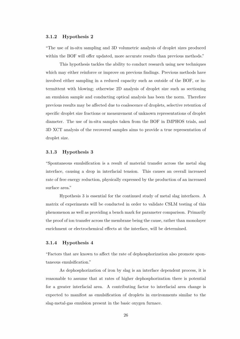
3.1.2 Hypothesis 2

“The use of in-situ sampling and 3D volumetric analysis of droplet sizes produced

within the BOF will offer updated, more accurate results than previous methods.”

This hypothesis tackles the ability to conduct research using new techniques

which may either reinforce or improve on previous findings. Previous methods have

involved either sampling in a reduced capacity such as outside of the BOF, or in-

termittent with blowing; otherwise 2D analysis of droplet size such as sectioning

an emulsion sample and conducting optical analysis has been the norm. Therefore

previous results may be affected due to coalescence of droplets, selective retention of

specific droplet size fractions or measurement of unknown representations of droplet

diameter. The use of in-situ samples taken from the BOF in IMPHOS trials, and

3D XCT analysis of the recovered samples aims to provide a true representation of

droplet size.

3.1.3 Hypothesis 3

“Spontaneous emulsification is a result of material transfer across the metal slag

interface, causing a drop in interfacial tension. This causes an overall increased

rate of free energy reduction, physically expressed by the production of an increased

surface area.”

Hypothesis 3 is essential for the continued study of metal slag interfaces. A

matrix of experiments will be conducted in order to validate CSLM testing of this

phenomenon as well as providing a bench mark for parameter comparison. Primarily

the proof of ion transfer across the membrane being the cause, rather than monolayer

enrichment or electrochemical effects at the interface, will be determined.

3.1.4 Hypothesis 4

“Factors that are known to affect the rate of dephosphorization also promote spon-

taneous emulsification.”

As dephosphorization of iron by slag is an interface dependent process, it is

reasonable to assume that at rates of higher dephosphorization there is potential

for a greater interfacial area. A contributing factor to interfacial area change is

expected to manifest as emulsification of droplets in environments similar to the

slag-metal-gas emulsion present in the basic oxygen furnace.

26

3.1.5 Hypothesis 5

“Spontaneous emulsification is initiated by perturbation and the potential this cre-

ates for reducing diffusion distance.”

Liquid interfaces are known to perturb. As such the produced heterogeneous

morphology of the interface creates an environment where the potential for transfer

of material across the interface is non-uniform. Impurity refinement in high tem-

perature systems is reportedly often restricted by mass transfer of material in either

bulk phase; the growth of a perturbation has the potential to remove or reduce this

kinetic restriction, drastically increasing the rate of free energy dissipation.

3.1.6 Hypothesis 6

“Spontaneous emulsification can be predicted from fundamental knowledge of the

system.”

Spontaneous emulsification is driven through the refining of material, and

the extent to which the two phases aid or resist intermixing. If variables such

as diffusion rates, viscosities and interfacial tension are known, the likelihood and

extent of emulsification should be predicable via an appropriate method.

3.1.7 Hypothesis 7

“Within a given system there is a critical point at which the spontaneous emulsifi-

cation will begin to occur with respect to starting material composition.”

If spontaneous emulsification is driven by the transfer of material across the

interface of metal and slag, then there should be a critical inflection of behaviour

where the phenomenon does and does not occur. As such there should be energetic

accountability for the relief of increased global interfacial tension between the two

systems.

3.2 Hypothesis Approach

3.2.1 Hypothesis 1

Previous work [4] carried out by Tata Steel Europe scientists will be examined,

progressed and developed. This will involve combining quantitative data from the

27

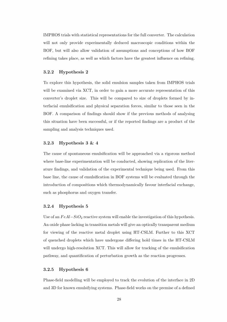
IMPHOS trials with statistical representations for the full converter. The calculation

will not only provide experimentally deduced macroscopic conditions within the

BOF, but will also allow validation of assumptions and conceptions of how BOF

refining takes place, as well as which factors have the greatest influence on refining.

3.2.2 Hypothesis 2

To explore this hypothesis, the solid emulsion samples taken from IMPHOS trials

will be examined via XCT, in order to gain a more accurate representation of this

converter’s droplet size. This will be compared to size of droplets formed by in-

terfacial emulsification and physical separation forces, similar to those seen in the

BOF. A comparison of findings should show if the previous methods of analysing

this situation have been successful, or if the reported findings are a product of the

sampling and analysis techniques used.

3.2.3 Hypothesis 3 & 4

The cause of spontaneous emulsification will be approached via a rigorous method

where base-line experimentation will be conducted, showing replication of the liter-

ature findings, and validation of the experimental technique being used. From this

base line, the cause of emulsification in BOF systems will be evaluated through the

introduction of compositions which thermodynamically favour interfacial exchange,

such as phosphorus and oxygen transfer.

3.2.4 Hypothesis 5

Use of an FeAl−SiO2 reactive system will enable the investigation of this hypothesis.

An oxide phase lacking in transition metals will give an optically transparent medium

for viewing of the reactive metal droplet using HT-CSLM. Further to this XCT

of quenched droplets which have undergone differing hold times in the HT-CSLM

will undergo high-resolution XCT. This will allow for tracking of the emulsification

pathway, and quantification of perturbation growth as the reaction progresses.

3.2.5 Hypothesis 6

Phase-field modelling will be employed to track the evolution of the interface in 2D

and 3D for known emulsifying systems. Phase-field works on the premise of a defined

28

interface boundary; ideal for tracking its movement in space and time. Modelling of

the same systems investigated experimentally will allow for conversion from Fourier

time and space, to Cartesian space and relative times of reaction. The ability to

make this comparison will allow for cross interrogation of results to verify that the

driving forces within the model are similar to those in the physical systems.

3.2.6 Hypothesis 7

Variable initial alloy composition of 8, 5, 4, 3, 2, 1 and 0wt% aluminium in iron will

be used to observe interfacial phenomena in-situ. The development of automated

HT-CSLM and post-process image analysis will allow for quantification of observed

perturbation, necking and spontaneous emulsification levels. In addition an attempt

to verify any changes in behaviour via a free energy dissipation balance will be

investigated.

29

Chapter 4

Experimental Methods

The present work consists of three distinct experimental ventures:

1. Sequential inline sampling of a 6 ton pilot plant BOF.

2. The coupling of HT-CSLM, XCT and phase-field simulation

3. Post processing analytical techniques

4.1 Pilot Plant Based Experiments

The results chapter entitled “Calculating the macroscopic dynamics of the Gas/Met-

al/Slag Emulsion during steelmaking” builds on the initial findings of the European

Commission funded project “IMPHOS: Improved Phosphorus Refining”.

The groundings of the experiment are the sequential sampling of a 6 ton BOF

at the MEFOS site in Sweden. A robotic carousel was used to deliver a 7 height

sampling lance to the converter roughly two minutes apart through 24 blows.

The samples can be split into groups, where level 1 consists of bulk bath

material, 2 and 3 are at the interface level between the bulk steel bath and emulsion

phase, and 4-7 are at increasing height within the emulsion phase.

For the investigations in this work, chemical analysis of steel and slag phases

was required, along with time dependent off-gas composition and mass fraction of

each phase within a single sample.

In addition, unprocessed emulsion samples were used to briefly touch on the

droplet sizes within the emulsion phase; the data from which is used to give rudimen-

tal validation to an assumption within the investigation of percentage contribution

30

to decarburization of each zone within the BOF.

Further details of this programme of experimentation are presented within

the relevant results chapter.

4.2 High-Temperature Confocal Scanning Laser Microscopy

The HT-CSLM is a key tool used for the development of the presented results. The

equipment itself is depicted in figure 4.1. The main body consists of an elliptical

gold-coated chamber with a halogen bulb positioned in the lower focal point, and the

sample positioned in the upper focal point. The sample is held in place through the

extension of an alumina rod from the side of the chamber, through which an R-type

thermocouple is threaded, and subsequently fused to the underside of a platinum

ring positioned at the free end of the alumina rod. It is on this ring that the sample

is placed. IR radiation produced from the halogen bulb is then reflected from the

chamber walls and focused onto the sample. This results in possible heating rates

of up to 700 K min−1 and temperatures up to 1973 K.

UV Laser Head

Optics

High

Speed

Camera

High-Temperature Stage

Tensile-

Compression

Stage

Halogen Bulb Gas Inlet

Vacuum-

Exhaust

Outlet

Sample

Stage

Figure 4.1: The High-Temperature Confocal Scanning Laser Microscope. a) Showsa broader image of the instrument complete with both the high-temperature andtensile/compression stage. b) Shows the interior of the high temperature chamber.

The instrument is equipped with a rotary vacuum pump and a high-purity

argon gas feed (99.9999% purity) supply which is subsequently passed through a fur-

ther system of cold zirconium based getters, filters, drying chambers and a heated

getter at 623 K containing copper and magnesium turnings. This results in a con-

sistent oxygen level <2 ppb. The instrument is also linked to a switched helium

31

source for quenching, enabling cooling rates at steel/slag solidification temperatures

of 3000 K min−1.

Above the heating chamber there is a UV laser positioned with pin hole

focusing apertures. The UV laser is used so that the IR radiation from both the

bulb and heated sample do not interfere with the image produced. The laser can be

controlled both manually and automatically through use of a third-party program.

This allows for reactive imaging in relation to the ongoing observations of a study

being carried out, as well as a predetermined focusing regime which will allow for

tracking of the horizontal plane within the sample being viewed. As a result it is

possible to assess surface topologies of a sample, as well as tracking a system moving

in the z-direction.

The nature of the confocal optics allows for high resolution in the z-direction

imaging plane. For the in-situ spontaneous emulsification observations in the chapter

entitled “Spontaneous Emulsification as a Function of Material Exchange” it was

necessary to follow the droplet with accuracy to enable quantification of surface

area. As a result both the z-focal positioning and aperture of the laser were rastered

to enable a greater depth of field, but also the accurate imaging of a 2D plane within

the sample. The video capture and temperature programming is controlled through

the HiTOS software package.

The individual experimental set-ups for each experiment are described within

the relevant chapters.

4.3 X-ray Computed Tomography

XCT has been used for medical purposes for a reasonable period of time now; how-

ever the last 25 years has seen the technique find application in industrial metrology

for non-destructive testing and measurement. Full 3D evaluation of objects with no

physical modification or destruction to the original part is possible.

The machines used in this study consist of an X-ray cone beam source and

detector positioned at either side of a rotational stage upon which the object for

inspection is placed as shown in figure 4.2. The source produces X-rays which

pass through the sample, resulting in an image produced on the detector screen.

Locations where a higher number of X-rays have been attenuated by the object

32

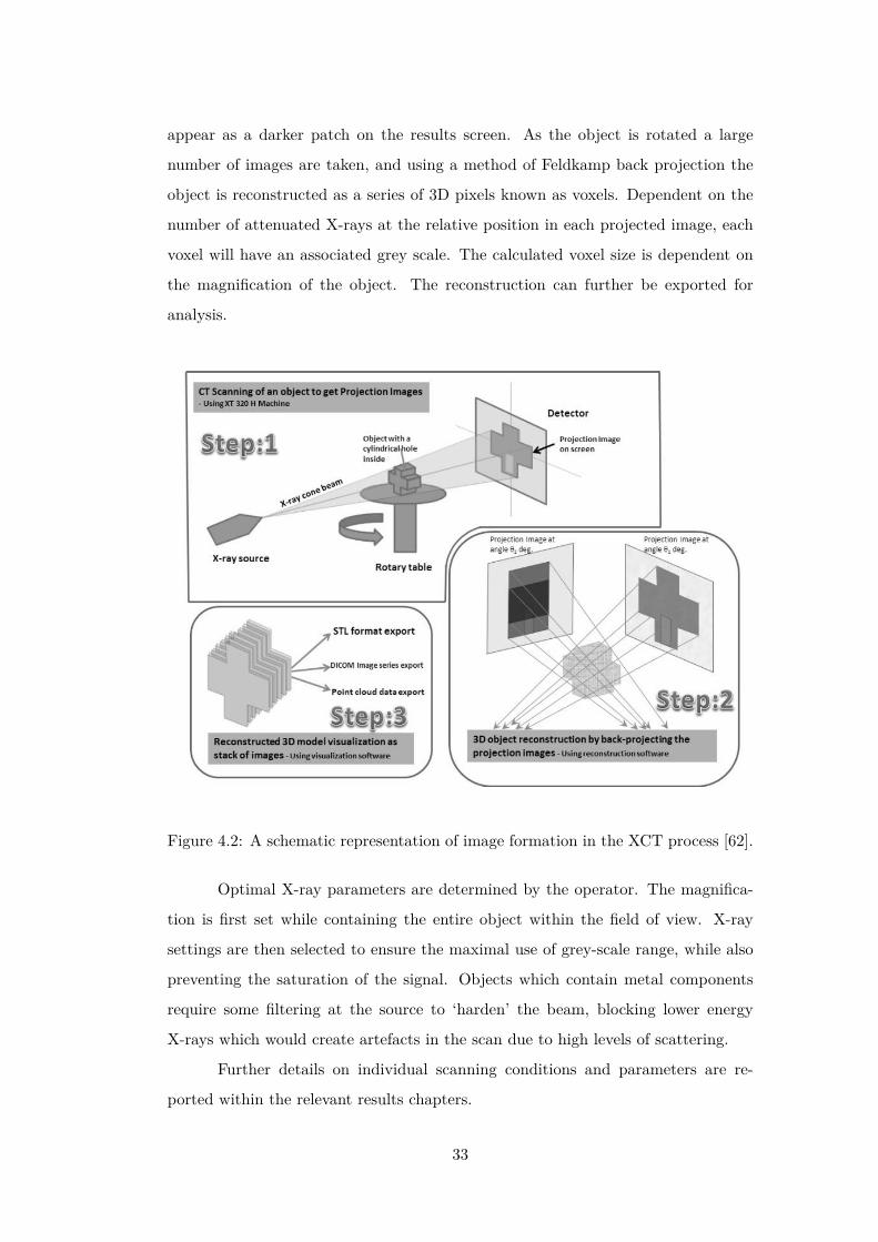
appear as a darker patch on the results screen. As the object is rotated a large

number of images are taken, and using a method of Feldkamp back projection the

object is reconstructed as a series of 3D pixels known as voxels. Dependent on the

number of attenuated X-rays at the relative position in each projected image, each

voxel will have an associated grey scale. The calculated voxel size is dependent on

the magnification of the object. The reconstruction can further be exported for

analysis.

Figure 4.2: A schematic representation of image formation in the XCT process [62].

Optimal X-ray parameters are determined by the operator. The magnifica-

tion is first set while containing the entire object within the field of view. X-ray

settings are then selected to ensure the maximal use of grey-scale range, while also

preventing the saturation of the signal. Objects which contain metal components

require some filtering at the source to ‘harden’ the beam, blocking lower energy

X-rays which would create artefacts in the scan due to high levels of scattering.

Further details on individual scanning conditions and parameters are re-

ported within the relevant results chapters.

33

XCT scanning and subsequent 3D volume analysis for the current reportings

were carried out by Dr Jason Warnett.

4.4 Phase-Field Simulation

To model the droplet behaviour in the experimental emulsification systems, the dual

effects of non-Newtonian rheology and the moving interface had to be considered.

Navier-Stokes equations were employed to model the unsteady, viscous, in-

compressible and immiscible two-fluid systems in two- and three-dimensional space:

ρi(δuiδt

+ ui.∇ui) = −∇pi +∇.[ηi(∇ui +∇uTi )] + SF in Ωi (4.1)

and

∇.Ui = 0 in Ωi (4.2)

where ρi(x, t) refers to the density, ui(X, t) = (u1(x, t), u2(x, t), u3(x, t)) de-

notes velocity, ρi(X, t) and ηi(X, t) are the pressure and viscosity of fluids i = 1, 2,

respectively. The transcript T refers to transpose and Ω represents the domain of

each fluid. SF represents surface tension force. Normally this surface tension is

considered a singular force and is defined as SFsing = −σκΓn where σ is the sur-

face tension coefficient and κ is the mean curvature of the interface [62] and δΓ is

the surface delta function [70]. In order to make the mathematical definition of

surface tension compatible with the phase-field formalism, a regular SF force was

employed. It is then possible to implement the Laplace-Young calculation [71] at

the exact interface boundary using a continuum surface force. This converts the

surface tension jump condition across the interface into an equivalent volume force

to which the Navier-Stokes equations are added. Thus SF is defined as:

SF = 6√

2εσ∇.(|∇c|2I −∇c⊗∇c) (4.3)

where ε is the gradient coefficient, c is the composition, I is the identity

matrix and (∇c⊗∇c)ij = δcδxi

δcδxj

is the usual tensor product.

Density and viscosity are defined as linear functions of the phase-field [72]

and harmonic interpolation and linear interpolation for the density and viscosity are

34

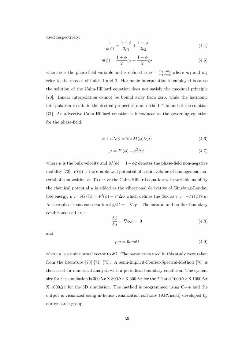
used respectively:1

ρ(φ) = 1 + φ

2ρ1+ 1− φ

2ρ2(4.4)

η(φ) = 1 + φ

2 η1 + 1− φ2 η2 (4.5)

where φ is the phase-field variable and is defined as φ = m1−m2m1+m2

,where m1 and m2

refer to the masses of fluids 1 and 2. Harmonic interpolation is employed because

the solution of the Cahn-Hilliard equation does not satisfy the maximal principle

[70]. Linear interpolation cannot be bound away from zero, while the harmonic

interpolation results in the desired properties due to the L∞-bound of the solution

[71]. An advective Cahn-Hilliard equation is introduced as the governing equation

for the phase-field:

φ+ u.∇φ = ∇.(M(φ)∇µ) (4.6)

µ = F ′(φ)− ε2∆φ (4.7)

where µ is the bulk velocity and M(φ) = 1−φ2 denotes the phase-field non-negative

mobility [72]. F (φ) is the double well potential of a unit volume of homogenous ma-

terial of composition φ. To derive the Cahn-Hilliard equation with variable mobility

the chemical potential µ is added as the vibrational derivative of Ginzburg-Landau

free energy, µ := δG/δφ = F ′(φ)− ε2∆φ which defines the flux as T := −M(φ)∇µ.

As a result of mass conservation δφ/δt = −∇.T . The natural and no-flux boundary

conditions used are:δφ

δn= ∇φ.n = 0 (4.8)

and

T .n = 0onδΩ (4.9)

where n is a unit normal vector to δΩ. The parameters used in this study were taken

from the literature [73] [74] [75]. A semi-Implicit-Fourier-Spectral-Method [76] is

then used for numerical analysis with a periodical boundary condition. The system

size for the simulation is 300∆x X 300∆x X 300∆x for the 2D and 1000∆x X 1000∆x

X 1000∆x for the 3D simulation. The method is programmed using C++ and the

output is visualized using in-house visualization software (ARVisual) developed by

our research group.

35

Dr Alireza Rahnama was responsible for formulating and coding the phase-

field simulation.

4.5 Additional Analytical Techniques

4.5.1 Scanning Electron Microscopy (WDS and SIMS)

Scanning electron microscopy (SEM) is the bread and butter of materials character-

ization today. The technique was applied in the research for the clarification of the

stock Fe− P alloy. The SEM instrument used for this project was the Sigma-Zeiss

model, a field-emission gun SEM (FEG-SEM). In addition to the imaging capability

of the instrument, time of flight-secondary iron mass spectroscopy (TOF-SIMS), and

wavelength dispersive spectroscopy (WDS) were used for the analysis of oxygen and

phosphorus content respectively.

4.5.2 XRF, ICP and LA-ICPMS

X-ray Florescence (XRF) was used for chemical analysis of the synthetically pro-

duced slags. The model of equipment used in this project was the “Thermo Scientific

ARL PERFORM’X Sequential 2.5kW XRF Spectrometer”. A bead of slag is loaded

into the sample holder in the XRF machine and the chamber is vacuumed and the

sample ionized with X-rays. Analysis of fluorescent X-rays and their intensities were

then compared against intensity profiles from certified calibration reference material,

which had been prepared under the same conditions as the experimental samples.

XRF OXSAS software was then used to calculate the average composition from 3

identical scans.

Inductively coupled plasma mass spectroscopy (ICP) was used to determine

stock alloy compositions used in the HT-CSLM experiments in this study. For

the instrument used in this project a portion of the sample is dissolved and then

introduced to the plasma source through a spray chamber. The sample undergoes

ionization from the plasma source and is then focused into a quadrupole region

by single iron lenses. This focuses the beam of ions for chemical modification to

eliminate interference. Once in the mass spectroscopy chamber, ions are separated

via mass to charge ratios and picked up by the detector.

Laser ablation inductively coupled plasma mass spectrometry (LA-ICPMS)

36

differs from traditional ICP in that a laser is used to directly ablate some of the

sample surface which is then passed into the quadrupole/mass spectrometry detector

series. This technique was used to confirm the data collected via WDS for some

samples. LA-ICPMS is generally regarded as a very accurate chemical analysis

technique.

4.6 Materials

Table 4.1 contains their heat number and starting “hot metal” composition for each

IMPHOS heat used for calculating the macroscopic dynamics.

Table 4.1: IMPHOS heats and their starting “hot metal” compositions collected byspark optical emission spectrometry. [4].

Heat ID %C %Si %Mn %P %SS1828 4.19 0.54 0.46 0.079 0.048S1829 4.07 0.51 0.46 0.085 0.044S1830 4.10 0.47 0.40 0.086 0.037S1831 4.16 0.46 0.44 0.095 0.038S1832 4.10 0.58 0.44 0.067 0.037S1833 3.94 0.44 0.44 0.070 0.042S1834 3.83 0.66 0.43 0.082 0.048S1835 4.04 0.60 0.44 0.084 0.047S1836 4.06 0.64 0.48 0.086 0.051S1837 3.90 0.59 0.42 0.094 0.051S1840 3.79 0.58 0.42 0.084 0.054S1843 4.04 0.56 0.42 0.089 0.043S1845 4.07 0.53 0.46 0.095 0.045S1846 4.16 0.55 0.43 0.087 0.043

The compositions of alloys and slags used in HT-CSLM experiments are given

in table 4.2 and 4.3 respectively.

37

Table 4.2: The compositions of all metallic alloys used in HT-CSLM experimentsmeasured using ICP (where all N levels are <0.001%.Alloy ID %Mn %P %Ni %Cr %Al %C %S %Oa1 0.011 0.201 0.003 0.002 0.002 0.0008 0.0012 0.0737a2 0.0003 0.0004 0.0001 0.0003 0.0005 0.004 <0.001 0.0034Fe −FeO

0.003 0.0004 0.0001 0.0003 0.0005 0.004 0.001 0.0034

Null 0.003 0.0004 0.0001 0.0003 0.0005 0.004 0.001 0.0034FeAl −SiO2

0.0002 0.0004 0.002 0.0005 7.87 0.0007 0.001 0.0038

0% Al 0.0003 0.0004 0.0001 0.0003 0.00005 0.004 0.001 0.00341% Al 0.0003 0.0004 0.002 0.0005 0.99 0.0011 0.001 0.00282% Al 0.0004 0.0004 0.001 0.0003 1.92 0.0006 0.001 0.00293% Al 0.0002 0.0004 0.002 0.0005 2.84 0.0011 0.002 0.00354% Al 0.0004 0.0004 0.002 0.0005 3.98 0.0007 0.002 0.00425% Al 0.0003 0.0003 0.002 0.0004 4.92 0.0009 0.002 0.00408% Al 0.0002 0.0004 0.002 0.0005 7.87 0.0007 0.001 0.0038

Table 4.3: The compositions of all slags used in HT-CSLM experiments measuredusing XRF.Slag ID %CaO %MgO %SiO2 %FeOt %P2O5 %CaO/SiO2 %Al2O3

S1 36.64 7.08 16.98 33.56 1.66 2.16 0S2 36.89 7.14 16.21 33.31 1.65 2.28 0S3 38.15 10.26 16.89 34.70 0.01 2.26 0S4 43.02 8.74 24.11 0 0 1.78 24.13Fe −FeO

36.89 7.14 16.21 32.31 1.65 2.28 0

Null 43.02 8.74 24.11 0 0 1.78 24.13FeAl −SiO2

36.17 0 23.11 0 0 1.57 38.53

38

4.7 Technical Approach

The above techniques combine to give a unique approach to the interrogation of the

project hypotheses.

The extensive experimental sampling and recording of data within the IM-

PHOS project offers a unique set of information to cohesively interrogate the re-

fining pathways present. The sequential multi-layered sampling offers the highest

time-resolved in-situ sampling of a BOF today, with the addition of the converter

process being able to continue while sampling takes place, there was the opportunity

to take samples more representative of the continuing process than ever before.

In addition the multiple heats, accurate reporting of processing parameters

and time-resolved off-gas analysis, gives the opportunity to truly see how process

parameters affect the distribution of refining contributions with the reported bulk

bath, hot zone and emulsion zones of the BOF.

The laboratory based techniques offer several advantages. HT-CSLM allows

for the controlled suspension of a metal droplet in a slag phase, which is able to heat

at relatively high rates ensuring close time proximity of slag and metal melting.

This offers the ability, along with in-situ observation of the slag melting, to report

a true t = 0 for interaction to occur. In addition HT-CSLM allows for the in-situ

observation of the phenomena when optically transparent slags are used. This is

necessary to truly appreciate how spontaneous emulsification progresses (for instance

in such an instantaneous manner for the higher FeAl content samples). Variation

in user application can have a significant effect upon HT-CSLM results, this is due

to effects of surface roughness on light radiation heating, required speed of image

focusing response and maintenance of the chamber environment. To develop this

technique it required signifcant investment of time and process improvment, for

example: Deducing the correct amount of slag to pack above and below the metal

droplet to avoid interaction with the crucible or floating of the metal on the slag

surface; maintenace and cleaning of both the HT-CSLM chamber and argon gas

(removal of oxygen down to ppt levels) in order to avoid contamination or the metal

droplet oxidizing before the reaction could take place; correct alighnment and trial of

the heating profile programming in order to attain the desired sample temperature

profile (as the control thermocouple is attached to the bottom of the sample stage,

39

not the sample itself); experties of focusing on a moving target (melting surface)

in order to gain image data from a near t=0 point; improvment of experimental

set-up to increase the homogenouity of temperature through the sample (through

use of saphire crucibles and sample location testing) to enable the molten droplet to

remain still enough for imaging; introducing helium gas as a quenching enviroment

in order to preserve molten morphologies to room temperature. The above lists

some of the major factors in controlling the HT-CSLM experiments in order to gain

the insights presented in this thesis. Although a significant amount of experimental

development was required, once a working proceedure was identified the experiments

became extreamly reliable.

In addition, the small sample size within the HT-CSLM allows for rapid

quenching of the sample by turning off the heat source and introducing an atmo-

sphere with higher thermal capacity (in the case of these experiments swapping from

argon to helium gas). This allows for reliable shape retention from liquid to solid

and thus ex-situ XCT can be applied. High-resolution XCT for well-defined phase

boundaries and spatial confidence requires long scanning times, giving limitation to

the ability of using the techniques in a high-throughput fashion.

XCT offers 3D calibrated analysis of the physical shape and size of each

phase within a sample. This is favourable compared to other techniques used in the

literature such as SEM or X-ray radiography as these only allow you to see either

a given cross section or the largest form of the droplet in all directions respectively.

There are obvious inherent issues with each of these.

Finally, phase-field modelling is unique in its depiction of the interface. As

experiments within this project are interface driven it is thus the chosen method.

Phase-field modelling offers the ability to track composition change, the tension of

the interface with respect to angular strain and the spatially dependent driving force

of reaction. These couple to give a good interpretation and visualization through

image output of the cause of spontaneous emulsification. The unavoidable issues

with phase-field modelling are the need to define an interface width (usually over

estimated) and the significant computational effort required.

40

Chapter 5

Calculating the Macroscopic

Dynamics of the

Gas/Metal/Slag Emulsion

During Steelmaking

5.1 Hypothesis to be Interrogated

Hypothesis 1: “Periods of greater dephosphorization in the BOF correspond to times

of greater interfacial area between slag and metal.”

Hypothesis 2: “The use of in-situ sampling and 3D volumetric analysis of

droplet sizes produced within the BOF will offer updated, more accurate results

than previous methods.”

These hypotheses present a platform to interrogate the environment within

the BOF and to quantify the nature of the transient slag/metal interface present in

the emulsion zone.

5.2 Introduction

Currently phosphorus levels are controlled through operation of the Basic Oxygen

Furnace (BOF); however this is a secondary function of the converter, whose main

job is decarburization (the reaction pathways shown in equations ?? and ??. As

41

a result processing parameters have to be balanced and inhibiting factors such as

oxygen removal and high temperatures occur which reduce the phosphorus refining

performance of the BOF.

The dephosphorization reaction consists of a series of potentially kinetic lim-

iting steps:

1. Transfer of phosphorus from bulk steel to slag/steel interface

2. Transfer of oxygen ions from bulk slag to slag/steel interface

3. Chemical reaction at slag/steel interface

4. Transfer of oxygen from slag/steel interface to bulk steel

5. Transfer of phosphate ions from slag/steel interface to bulk slag

As previously stated in the chapter entitled ”Underpinning Knowledge” it is

typically assumed the chemical reaction at the interface can be ruled out as rate

limiting due to the speed at which it takes place. As a result the rate is believed to

be predominantly controlled by the mass transfer of ions in either or both bulk metal

and slag [22] [77] [78]. The term “bulk metal” in this case refers to a region where

the material is compositionally constant in space and could be in the metal bath or

inside a metal droplet. This leads to a rate of dephosphorization dependent upon

metal packet size, and the time period required for that metal to refine. Therefore the

transient interfacial area is a macroscopic kinetically restricting factor for phosphorus

refining. The quiescent interface of the bulk bath is a small portion of the overall

metal/slag interface, as the emulsion phase of the BOF contains a dispersion of

metal packets/ droplets. Previous studies have investigated the range of what sizes

these droplets are [4] [51] [39] [40] [42] [43] [44] [46] [38]. However coupled with

this information it is important to know the percentage of metal accounted for in

the emulsion (% tap weight), the metal circulation rate within the emulsion (as this

affects localised diffusion gradients), and how long the metal remains in the emulsion

(residence time).

Residence times have been both modelled and calculated from blow sampling

in several previous studies. The residence time is defined as the period of time which

has lapsed between a “packet of metal” leaving the surface and re-entering the bulk

42

bath. Table 5.1 shows a summary of the previous reported residence times, the

author and the method of calculating/modelling the process.

The IMPHOS project was a European funded project to investigate the pro-

cess of phosphorus refinement in the BOS converter. A 6 ton converter was sampled

at systematic time intervals, simultaneously at selected levels throughout several

heats. This sampling procedure enabled metal collection and compositional anal-

ysis of the metal in the emulsion in addition to that in the bulk bath during an

un-interrupted blow. Using data from IMPHOS trials macroscopic dynamic factors

such as the mass of metal in the emulsion, the average residence time (ART) of

this metal, and the dynamic emulsion flow speeds can be calculated. The accurate

quantification of these parameters is vital to fully understanding and optimising

BOF refining. This chapter explores calculating macroscopic dynamics based upon

carbon mass balancing from realistically attainable plant data, whilst neglecting

previous widely accepted significant factors to still offer an accurate result.

43

Tabl

e5.

1:C

olla

tion

ofpr

evio

usly

repo

rted

resid

ence

times

,with

the

expe

rimen

tal/

mod

ellin

gte

chni

que

used

.A

utho

rM

etho

dof

Ded

uctio

nR

esid

ence

Tim

e(s

)Pr

ice

[38]

Gol

diso

tope

trac

king

,pla

ntm

easu

rem

ent

120±

30

Koz

akev

itch

[51]

Plan

tm

easu

rem

ent

ofca

rbon

and

phos

phor

usle

velp

redi

ctio

nsin

met

al60

-120

Broo

kset

al[5

2]R

evise

dpr

edic

tion

todr

ople

ttr

ajec

tory

mod

el,

with

bloa

ted

drop

let

effec

ts.

On

ade

fined

15%

FeO

and<

85%

gas

fract

ion

20-8

0

Dog

anet

al[5

4][7

9]Si

mila

rto

Broo

kset

al,b

ut14

-30%

FeO

cont

ent

scre

ened

and

afix

edga

sfra

ctio

nof

80%

0.4-

45

Qin

g[5

3]3-

Dtw

oph

ase

(mer

cury

/gly

cerin

e)m

odel

1-40

Scho

opet

al[8

0]C

alcu

late

dfro

ma

kine

ticm

odel

and

chem

ical

anal

ysis

ofin

dire

ctpl

ant

sam

ples

∼60

44

5.3 Experimental

5.3.1 Heat Characteristics

This chapter interrogates 14 of the 25 heats conducted during the IMPHOS trials;

these heats were selected due to consistently reliable data sets, and the inclusion

of varying factors such as sampling time and hot metal silicon content. The heats

included are: S1828-S1837, S1840, S1843; S1845 & S1846, the nomenclature for

heat naming has been kept the same as the original IMPHOS report for ease of

reference [4].) The IMPHOS report is publically available and can be found on the

website for the European Commission.

The nominal composition for hot metal used in the trial is given in Table

5.2 and is near “normal” to hot metal outputs from the blast furnace in industrial

practice to increase relevance to application.

Table 5.2: Nominal start composition of hot metal used in IMPHOS trials.C mass% Si mass% Mn mass% P mass% S mass% Temp oC

4.75 0.45 or 0.6 0.45 0.085 0.03 1375

Further breakdown of individual heat conditions, and parameters such as ‘V’

ratio (mass% CaO/mass% SiO2), lime addition, lance height profiles and tapping

temperatures can be found in the European Commission report [4]. The author

recommends the data in the report is considered when evaluating the findings in the

present work.

IMPHOS trials were carried out at Swerea MEFOS, Sweden, with use of the

6 tonne pilot plant BOS converter. The converter has a lining of Magnesia-Carbon

(fired and fused) bricks, and is fitted with a single bath agitation tuyere blowing

nitrogen at a rate of 0.5Nm3min−1 and a water-cooled oxygen lance with a single

De-Laval nozzle (a convergent divergent nozzle; a pinched geometry to make an

asymmetric hourglass shape) blowing oxygen at 17Nm3min−1. A schematic of the

converter can be seen in figure 5.1 containing dimensions, sampling pot locations

and labelling of the terms used later in calculations.

Sampling of the converter was carried out via robotic delivery of specially

designed sample lances at 2 minute intervals throughout the blow. The lances consist

of an inner and outer structure of three mild steel bars, the inner being joined to

45

Figure 5.1: Schematic of MEFOS 6 ton converter with sample levels, dimensionsand Spv/Ev defined

the sides of inline sample pots, the outer joined to the sides of disc sample pot lids.

The lance is lowered into the converter through an opening in the top (with a slight

offset from the oxygen lance), with the lids in the closed position. Once lowered

into position, the outer three bars are retracted lifting the lids in-situ, allowing the

sample pots to fill. The lids were then closed after 3 seconds for all heats in this

study, apart from S1844, S1845 and S1846 where the lids closed after 3.5, 4 and 5

seconds respectively. The lances are then retracted from the converter, the lance

carousel rotates and the next lance is lowered after 2 minutes.

A small flake of each sample was extracted (for SEM analysis) after the full

sample was weighed. Each sample was then passed three times through a small

hammer mill. The material was then magnetically separated by hand-held magnet.

The now magnetic and non-magnetic fractions were weighed separately, and

chemically analysed via spark OES. The original IMPHOS report used this to sep-

arate the heats into 5 characteristic phosphorus refining profiles. A full collation of

46

IMPHOS sample chemical analysis can be seen in the report.

5.3.2 Model of BOS Converter for Calculating Macroscopic Dy-

namics

Initial Analytical Input

The method of calculation used in this thesis has a significantly different assumption

from that previously assumed in that sampling was linearly dependant on sample

pot opening times. It has now been assumed that the sampling of the converter was

instantaneous upon opening of the submerged sample pots, and the content of the

pot does not change with time.

The reason for this assumption is that upon inspection of the amount of

material collected in sample pots, as a function of sample pot opening time, longer

opening times lay within the spread of data produced by the normal three second

sampling time for this experiment. If sampling was to depend upon the pot opening

time, it would be expected that a trend would exist where the average metal collected

per pot per heat would increase with sample pot opening time.

Along with this change in sampling interpretation, a new method of modelling

the macroscopic dynamics has been proposed which relies heavily on quantified off-

gas analysis. Off-gas analysis is notorious for being inaccurate for full converter

analysis. To minimise potential error a mass balance has been carried out between

the mass of carbon lost between input and output hot metal, and that detected in

the off-gas.

From the carbon mass balancing a discrepancy of up to around 13% can be

seen, yet in most cases reasonable agreement is seen. To combat this discrepancy,

off-gas carbon detection is given a correction variable which uniformly distributes

the discrepancy across a heat’s blow time.

Method of Macroscopic Dynamics Calculation

The model created in this study uses output analysis from IMPHOS trials [4], such

as metal masses, chemical compositions and converter parameters. The main process

is an iterative carbon mass balancing between elemental analysis of emulsion zone

metal, and that of the bulk bath metal. Carbon mass balancing is used due to

the off gas detection offering a higher time resolution sampling in refined material,

47

as opposed to using phosphorus or silicon removal which would only be correlated

to the less frequent 2 minute slag sampling. Also decarburization continues to a

measureable point throughout the entire blow, where as other impurities are heavily

refined earlier, and change little towards the end. Firstly the overall mass of metal

in the emulsion zone is calculated through ratio scale up between sample volume

and converter volume. The carbon mass balancing of this metal with the timeline of

bulk bath composition in the same mass of metal is then used to calculate the ART.

Finally a relationship between mass of metal collection and its period of residence

is used to calculate metal circulation rate.

Equations 5.1 - 5.6 show the necessary steps for calculating the mass of metal

in the emulsion, the ART of metal in the emulsion and the metal circulation rate

within the emulsion.

Key assumptions beyond those previously stated are:

• The emulsion phase is solely responsible for decarburization. In this study the

emulsion phase is defined as levels 4-7 in the IMPHOS converter. Although it

is known that there are contributions from the bulk bath, and accelerated rates

from the hot zone (the area of oxygen jet impact on the metal bath surface),

this was deemed a reasonable working assumption due to the known high rates

of carbon removal in the emulsion type phase, a check of the validity of this

assumption is offered after the discussion. As such, levels 1-3 are considered

bulk bath/interface samples and above level 7 the density of slag is assumed

to be such that refining potential would be greatly reduced (a foam).

• The population (mass) of metal in the emulsion was consistent and remained

constant throughout the time period covered by the calculated ART unless

the calculated ART spanned two sampling points, upon which a regression of

change was factored into the calculation. This assumption was necessary in

order to perform the calculation and should be evaluated for each individual

point as to its reliability. An indication as to its reliability may be to assess

the change in metal circulation rate over the relevant time period.

• Sampling was a fair representation of environment throughout the full hori-

zontal plane of the converter. This assumption is not strictly accurate in the

vicinity of the main lance and the wall of the converter, but it is adopted be-

48

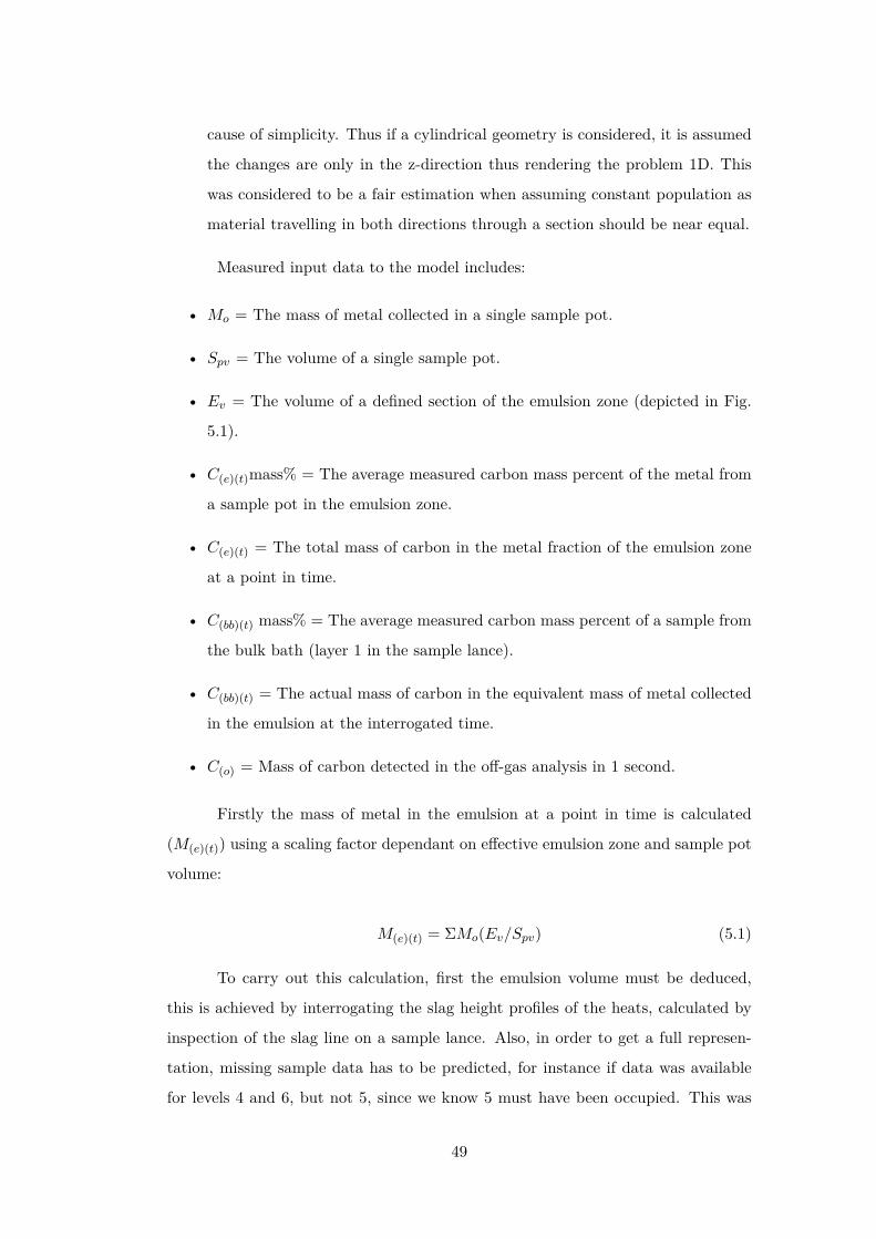
cause of simplicity. Thus if a cylindrical geometry is considered, it is assumed

the changes are only in the z-direction thus rendering the problem 1D. This

was considered to be a fair estimation when assuming constant population as

material travelling in both directions through a section should be near equal.

Measured input data to the model includes:

• Mo = The mass of metal collected in a single sample pot.

• Spv = The volume of a single sample pot.

• Ev = The volume of a defined section of the emulsion zone (depicted in Fig.

5.1).

• C(e)(t)mass% = The average measured carbon mass percent of the metal from

a sample pot in the emulsion zone.

• C(e)(t) = The total mass of carbon in the metal fraction of the emulsion zone

at a point in time.

• C(bb)(t) mass% = The average measured carbon mass percent of a sample from

the bulk bath (layer 1 in the sample lance).

• C(bb)(t) = The actual mass of carbon in the equivalent mass of metal collected

in the emulsion at the interrogated time.

• C(o) = Mass of carbon detected in the off-gas analysis in 1 second.

Firstly the mass of metal in the emulsion at a point in time is calculated

(M(e)(t)) using a scaling factor dependant on effective emulsion zone and sample pot

volume:

M(e)(t) = ΣMo(Ev/Spv) (5.1)

To carry out this calculation, first the emulsion volume must be deduced,

this is achieved by interrogating the slag height profiles of the heats, calculated by

inspection of the slag line on a sample lance. Also, in order to get a full represen-

tation, missing sample data has to be predicted, for instance if data was available

for levels 4 and 6, but not 5, since we know 5 must have been occupied. This was

49

done by fitting of a regression given by a full data set within IMPHOS trials with

similar known results. The appropriate regression is taken from a heat with similar

characteristics (sample sizes, and known distribution) and from the same time point

as the sample set with missing data. There is strong consistency in these profiles,

the match should give a realistic result.

Next the mass of carbon in the overall emulsion metal at a point in time

must be calculated (C(e)(t)) with use of a measured carbon mass percent of metal,

and scaled metal content of the emulsion:

C(e)(t) = Σ(Mo(Ev/Spv)/100)C(e)(t)mass% (5.2)

The mass of carbon in the bulk bath is now calculated as a function of time

for the same mass of metal as was found in the emulsion at time (t). This is done

by using the measure of carbon mass% of bulk bath metal throughout the blow and

the scaled mass of metal in the entire emulsion (C(bb)):

C(bb)(t) = (M(e)(t)/100)C(bb)(t)mass% (5.3)

It is now possible to add off-gas carbon detection values to the emulsion

metal carbon weight, in 1 second steps back in time from the sampling point. This

time-step carbon addition will intersect the local linear regression of analysed bulk

bath carbon content for the corresponding heat, as such:

C(bb)(t−tr) = C(e)(t) + Σni=oC(o)i (5.4)

Where C(o) is the mass of carbon, detected in the off gas in the nth second,

prior to sampling. The ART of all metal in the emulsion at time t in seconds is (tr):

tr = n (5.5)

This includes metal recently ejected from the bulk bath, the metal soon to

re-enter and all points in-between. Given the units of M(e)(t) (kg), and tr (s), it is

now possible to calculate the metal circulation rate (MCR) within the emulsion as

defined previously by Millman et al [69]:

50

MCR = M(e)(t)/tr (5.6)

5.3.3 X-ray Computed Tomography

Flakes of emulsion in solidified form from four different samples were scanned us-

ing X-ray Computed Tomography (XCT) for 3D observation of the steel in slag.

Furthermore this could be segmented to determine the position, size, volume and

surface area of each droplet contained within the slag. From the relatively uniform

distribution of pores and metal droplets through the samples it is expected the sam-

ples solidified rapidly (if a slow solidification took place it would be expected that

the different phases in a sample would have separated by density to a large extent,

this behaviour was not seen), as such the ex-situ investigation of the droplet sizes

and distribution is a good representation of the original environment.

The sample is placed on a rotating turntable between the source and detector.

The scanner used in this study was the Nikon XT 225/320 with the parameters

listed in Table 5.3. As X-rays traverse the sample they are either attenuated or pass

through resulting in a grey-scale radiograph on the screen. Numerous images are

taken through 360 degrees which are then reconstructed into a 3D volume through

the process of filtered back projection. The volume consists of a number of 3D pixels

called voxels with an associated grey value between 0 and 65535, proportional to

the attenuation of the material. Validation of the instrument’s accuracy has been

reported by Kumar et al [81].

Table 5.3: XCT scanning parameters used for the interrogation of solid emulsionshards removed from the sampling pots.

Voltage (kV) 180Current (micro A) 24

Exposure (s) 2.8Filter (Cu, mm) 0.5# Projections 3200

Voxel size (microns) 41

51

5.4 Results

The % tap weight (the amount of metal in the emulsion as a percentage of final

tap weight), ART and metal circulation rate within the emulsion at a point in time

have been calculated for 14 heats from a 6 ton pilot plant basic oxygen furnace. The

highest average %Tw in the emulsion being 31.07%, and the highest average ART

being 69 s; both of which occur in heat S1835. The highest average metal circulation

rate is that of S1837 being 305.41 kg s−1. Much larger variation is seen in the MCR

of blows than that of tr and %Tw . Table 5.4 shows the overall averages of all three

parameters, and their respective standard deviation to give an idea of cross heat

differences.

Table 5.4: Overall average and SD of %Tw, tr, and MCR for all blows.Overall Average Overall Average Overall Average

% Tw tr s MCR kg s−1

Mean Average 21.30 39 87.48Standard Deviation 6.40 16 72.44

For the purposes of this discussion the selected IMPHOS heats have been

split into three groups based on their computed ART profiles, these groupings are

qualitative and a device to aid presentation and discussion of results in the thesis,

the author is not stating it is possible to categorise all BOF profiles coherently into

one of the three groups presented here. The three groups are: “Mid blow inflection”

where the profiles show a raised and sustained relatively high ART through early

blow, followed by a drastic decrease around the middle period of the blow, with the

ART then staying low for the remainder of the blow; “High start then fluctuation”

when profiles show a large rise in ART up to 6 minutes into the blow, this peak

then rapidly decreases, followed by smaller fluctuations up and down in ART for

the remainder of the blow; “Residual Heats” show profiles unfitting to the previous

two groupings, these can be from an increased sustained high ART, to peaking

mid blow, or even a very low ART profile throughout the entire blow. There is no

correlation between these groupings and the operating conditions, input parameters

or measured output data from the experimental trial. Similarly scales of the different

grouping graphs that follow are different in the y-direction due to significantly varied

numerical results and the need to keep profile differences clear within a single sub-set.

52

5.4.1 Amount of Metal in the Emulsion

The amount of metal suspended in the emulsion is given as a percentage of the final

tap weight, rather than the input hot metal mass. This is due to FeO production

and sublimation of Fe material during a blow, resulting in a reduced possible mass

as the process continues. This is given as a function of blow time in figure 5.2.

5.4.2 Average Residence Time in the Emulsion

It should be noted these calculations are ART for packets of metal in the emulsion.

When the process is considered it is correct to propose that the spread of residence

times is variable from the calculated average through to a near zero second residence

time, for instance some material will re-enter the bulk bath almost as soon as it

leaves. Therefore residence time of individual packets of metal will be greater than

the average calculated. This should be taken into account when interpreting the

given ART, the defining of the greatest divergence from the calculated ART (min

and max) is however beyond the scope of this work. The ART as a function of blow

time is given in figure 5.3.

5.4.3 Metal Circulation Rate in the Emulsion

The speed of movement affects the end of blow results as apposed to a significant

drop in the mass of metal moving. With the exceedingly high rates seen in the last

2 minutes of the blow within the converter emulsion it is important to consider two

things; the first thing to note from the results of metal circulation rate is the graph

gives the illusion of a sustained rate up until the very high end-blow values, seen

in figure 5.4. Secondly, the metal circulation rates reported are an average of the

overall emulsion, much as the reported residence times; individual packets of metal

may be moving much faster or slower than the times calculated here.

5.4.4 XCT Results of Slag/Gas/Metal Emulsion Samples

An example 2D orthoslice of the resulting volume can be seen in figure 5.5 where the

bright white areas are metal droplets, the light grey areas slag material and black

areas porosity. As can be seen in the image the attenuation, and hence grey value, of

the slag is much lower than the steel, allowing for simple segmentation using the Otsu

53

Figure 5.2: The amount of metal in the emulsion as a percentage of final tap weight.a) “Mid blow inflection” group, b) “High start then fluctuation” group, c) “Residualheats” group.

54

Figure 5.3: The average residence time as a function of blow time. a) “Mid blowinflection” group, b) “High start then fluctuation” group, c) “Residual heats” group.

55

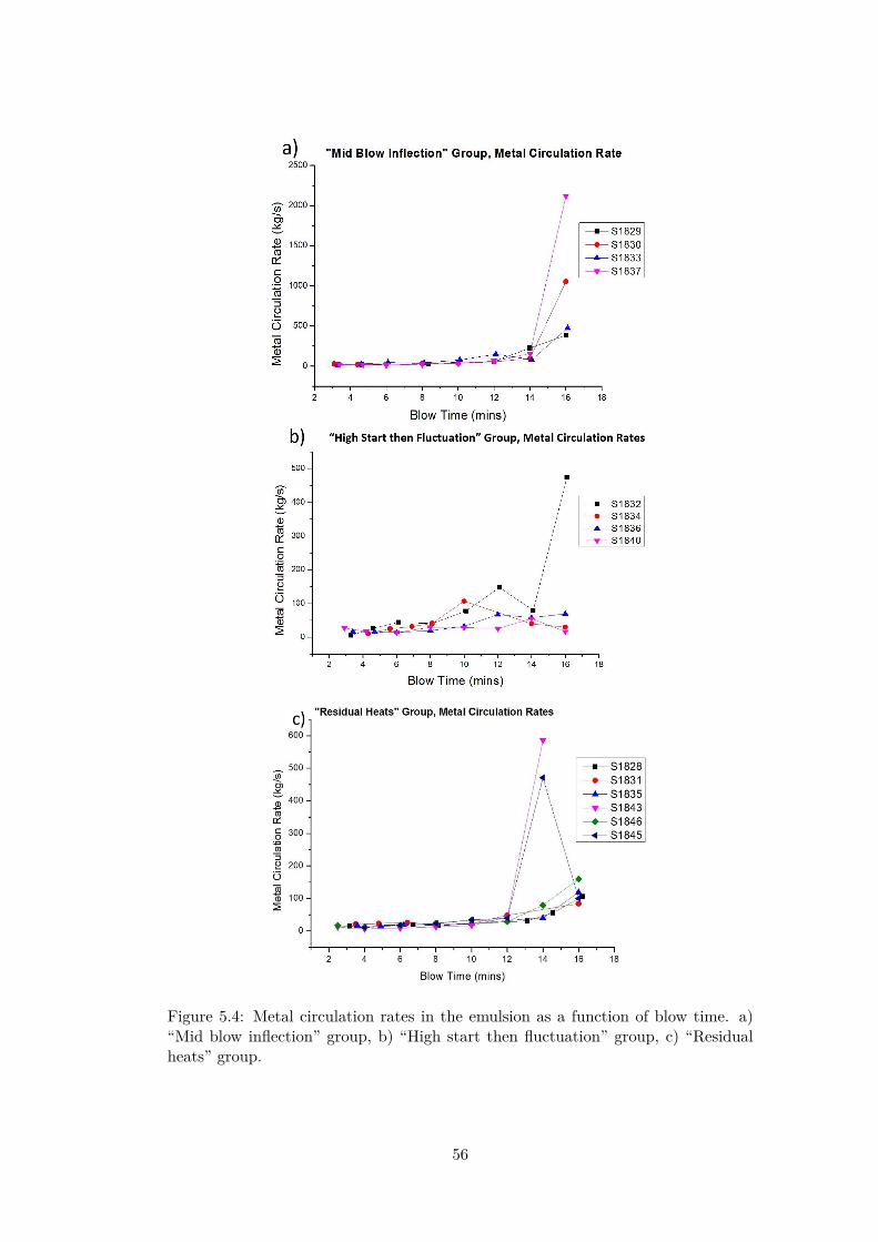
Figure 5.4: Metal circulation rates in the emulsion as a function of blow time. a)“Mid blow inflection” group, b) “High start then fluctuation” group, c) “Residualheats” group.

56

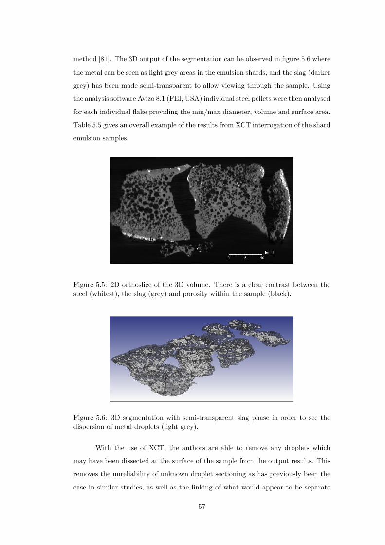
method [81]. The 3D output of the segmentation can be observed in figure 5.6 where

the metal can be seen as light grey areas in the emulsion shards, and the slag (darker

grey) has been made semi-transparent to allow viewing through the sample. Using

the analysis software Avizo 8.1 (FEI, USA) individual steel pellets were then analysed

for each individual flake providing the min/max diameter, volume and surface area.

Table 5.5 gives an overall example of the results from XCT interrogation of the shard

emulsion samples.

Figure 5.5: 2D orthoslice of the 3D volume. There is a clear contrast between thesteel (whitest), the slag (grey) and porosity within the sample (black).

Figure 5.6: 3D segmentation with semi-transparent slag phase in order to see thedispersion of metal droplets (light grey).

With the use of XCT, the authors are able to remove any droplets which

may have been dissected at the surface of the sample from the output results. This

removes the unreliability of unknown droplet sectioning as has previously been the

case in similar studies, as well as the linking of what would appear to be separate

57

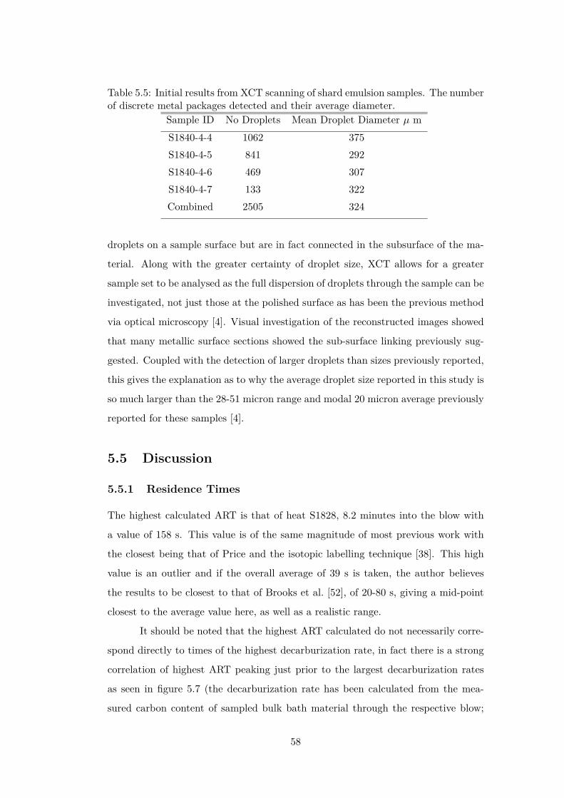
Table 5.5: Initial results from XCT scanning of shard emulsion samples. The numberof discrete metal packages detected and their average diameter.

Sample ID No Droplets Mean Droplet Diameter µ mS1840-4-4 1062 375S1840-4-5 841 292S1840-4-6 469 307S1840-4-7 133 322Combined 2505 324

droplets on a sample surface but are in fact connected in the subsurface of the ma-

terial. Along with the greater certainty of droplet size, XCT allows for a greater

sample set to be analysed as the full dispersion of droplets through the sample can be

investigated, not just those at the polished surface as has been the previous method

via optical microscopy [4]. Visual investigation of the reconstructed images showed

that many metallic surface sections showed the sub-surface linking previously sug-

gested. Coupled with the detection of larger droplets than sizes previously reported,

this gives the explanation as to why the average droplet size reported in this study is

so much larger than the 28-51 micron range and modal 20 micron average previously

reported for these samples [4].

5.5 Discussion

5.5.1 Residence Times

The highest calculated ART is that of heat S1828, 8.2 minutes into the blow with

a value of 158 s. This value is of the same magnitude of most previous work with

the closest being that of Price and the isotopic labelling technique [38]. This high

value is an outlier and if the overall average of 39 s is taken, the author believes

the results to be closest to that of Brooks et al. [52], of 20-80 s, giving a mid-point

closest to the average value here, as well as a realistic range.

It should be noted that the highest ART calculated do not necessarily corre-

spond directly to times of the highest decarburization rate, in fact there is a strong

correlation of highest ART peaking just prior to the largest decarburization rates

as seen in figure 5.7 (the decarburization rate has been calculated from the mea-

sured carbon content of sampled bulk bath material through the respective blow;

58

it is noted that the decarburization rate profiles show strong similarity within the

groups that have been defined by residence time performance, indicating a significant

link between the two). This makes sense as the decarburization rates are calculated

from the bulk bath measurements. As the refining takes place in the high residence

time droplets, a time-lapse close to the previously measured residence time would be

required in order to notice this effect. As an example S1837 has a peak in ART at

6 minutes followed by a peak in decarburization at 8 minutes. As ART is over 120

seconds at 6 minutes, it is understandable that the higher decarburization perfor-

mance is not expressed until later into the blow when these longer exposed packets of

metal have had time to recombine with the bulk bath. Thus it is strongly suggested

high residence times lead to higher decarburization rates. This is in agreement with

the work by Brooks [52], as the initial trajectory modelling carried out was given a

correction of transient droplet density due to decarburization reported by Molloseau

and Fruehan [82], resulting in the previously reported values by Brooks.

There is a visible correlation between points of higher ART and higher de-

phosphorization rates, as shown in figure 5.8 (the dephosphorization rate has been

calculated from the measured phosphorus content of sample bulk bath material

through the respective blow; it is noted that dephosphorization rate profiles show

less agreement with the residence time groupings than decarburization, however

there are still more common profile trends within each group). This correlation is

seen in the early blow with factors such as unfavourable temperature rise, removal

of FeO from the slag by decarburization and a reduction in phosphorus partition

gradient becoming increasingly unfavourable through the blow.

If the accepted strong link of high decarburization rates inhibiting dephos-

phorization are considered and taken into account when observing the given profiles,

it is arguably seen that dephosphorization rates are slightly higher at periods of

higher ART. This should be understood to be due to a larger effective interfacial

area between slag and metal, which aids in dephosphorization due to the nature of

phosphorus refinement through interfacial exchange. Not only is there a potential

for greater numbers of droplets in the emulsion phase at higher ART (assuming

constant droplet formation), the individual droplets are in contact with the slag for

a longer period of time, allowing for reactions between the two phases to occur for

longer and impurities to gain a closer phase balance to thermodynamic equilibrium.

59

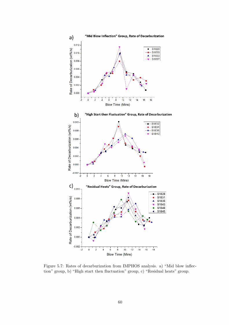
Figure 5.7: Rates of decarburization from IMPHOS analysis. a) “Mid blow inflec-tion” group, b) “High start then fluctuation” group, c) “Residual heats” group.

60

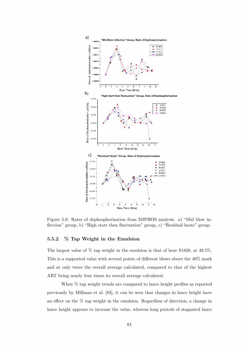
Figure 5.8: Rates of dephosphorization from IMPHOS analysis. a) “Mid blow in-flection” group, b) “High start then fluctuation” group, c) “Residual heats” group.

5.5.2 % Tap Weight in the Emulsion

The largest value of % tap weight in the emulsion is that of heat S1828, at 49.5%.

This is a supported value with several points of different blows above the 40% mark

and at only twice the overall average calculated, compared to that of the highest

ART being nearly four times its overall average calculated.

When % tap weight trends are compared to lance height profiles as reported

previously by Millman et al. [83], it can be seen that changes in lance height have

an effect on the % tap weight in the emulsion. Regardless of direction, a change in

lance height appears to increase the value, whereas long periods of stagnated lance

61

height tend to cause a trend back towards a minimum of around 10% (most values

are above this after the initial 2 minute calculation).

It is difficult to interpret the effects of different levels of metal mass in the

emulsion upon refining output directly, as without information on size distribution

the effect on surface area and mass transport times are effectively unknown. Further

work on IMPHOS data is planned to deliver better understanding in this area.

5.5.3 Metal Circulation Rates

The metal circulation rates have an apparent vast range. The highest value being

2,120.39 kg s−1 from heat S1837 which is an outlier from the majority of values

which are below 150 kg s−1. This value is partially due to the calculated ART being

the only value computed for the parameter below one second, as a result effectively

doubling the % tap weight in order to calculate metal circulation rate. As there is

little agreement in % tap weight values in end blow, this trend of high MCR towards

the end of the blow can be attributed to a reduction in ART. This effect is not seen

in early blow where residence times are also ‘low’ because effects such as significantly

lower masses of metal in the emulsion are also playing a role causing the effect to

be reduced due to the nature of the model.

This is understandable due to reduction in metal droplet bloating from de-

carburization; the smaller higher-density metal packages would be able to penetrate

through the slag medium with greater ease. Also when events such as slag layer

collapse are considered, along with the sampling technique where only samples sub-

merged in the slag layer are considered, it is unsurprising these circulation rates are

so high when a consistent ejection of material from the bulk bath is coupled with

a reduction in emulsion zone volume. It is also possible that due to the reduced

effective emulsion zone, the assumption of 100% decarburization in the emulsion

begins to break down, and the process is governed more strongly by bulk bath/slag

interactions and hot zone refining.

With the exclusion of the high end values, there is still a general trend for

MCR to increase as the blow time increases. This is a very slight increase and

may be accounted for through measurement of emulsion viscosity reduction due to

temperature increase (reducing slag viscosity), or higher gas fraction contribution

to the overall emulsion composition. Evidence for the latter is shown by the sudden

62

peak in decarburization shown in S1832 at 10 minutes into the blow, followed shortly

by a brief increase in metal circulation rate by almost 90 kg s−1.

5.5.4 Evaluation of Assumptions

The main observation that led to the diversion from the previously reported model

by Millman et al. [32] was sample collection time being shown to have no overall effect

on sample amount collected. As a result the method reported here was formulated.

It is believed by the author that the actual sampling time does not simply correlate

linearly with pot opening time, neither is it instantaneous; sampling is most likely

to be variable, dependent upon height within the converter. As such a sample from

level 4 would be more likely to be instantaneous as it is submerged in a denser, lower

gas fraction medium. Whereas a sample at level 7 (which would be in a possibly

more foam like medium) would have a continued filling for as long as the pot was

open.

The assumption of constant population is at this stage believed to be fair.

Metal circulation rates are not far from steady state, apart from an accountable rise

through the main blow. Also an evaluation in the change in amount of material

collected in consecutive samples shows mostly small variation.

Fair sampling of the converter is difficult to define. With the likelihood of in-

teractions such as streams of metal possibly hitting a sample pot when open (which

would be unrepresentative of the bulk emulsion phase), material over counting is

a possibility. The other side to this assumption is that the environment is similar

through a 2D horizontal sectioning of the converter. This environment will be signif-

icantly different close to the converter wall as opposed to at the oxygen lance in the

centre. Recent work by Sabah and Brooks [84] [85], using a scaled-down cold model

of water and air, has given significant support to this case. The authors intend to

evaluate these effects in further work. In addition it should be noted the IMPHOS

converter was only equiped with a single location for inert gas stirring in the base.

Industrial scale converters can contain many more locations for intert gas enty with

the amount and locations having significant effects of refining performance. It has

previoulsy been reported that bottom blowing can reduce the residence time of metal

droplets in the emulsion, due to a high gas fraction and thus reduced bouency (due

to reduce contact with slag for decarburization - bloating/haloing; a lower foam

63

density) [17].

Finally there is the assumption of 100% decarburization occurring within the

emulsion zone. This is known not to be accurate but offers an initial estimation to

construct this work. From the droplet size analysis carried out through XCT of the

samples from heat S1840, coupled with the use of a decarburization rate per unit

area and an average droplet size, it is possible to do a simple carbon mass balance to

evaluate this assumption. The solid density of 7.874 g cm−3, and a decarburization

rate of 7.5 x 10−7 mol s−1 a lower bound taken from Molloseau & Fruehan’s work [82]

are used (an over estimation due to the closest available data being that for a 1 g

droplet).

S1840 offers a mass of 554.82 kg metal in the emulsion and mean average

droplet diameter of 324 µm at the respective time. The calculated number of droplets

is 3.957 x 106. With an average droplet size ratio used the mass of CO2 generated

per second for one droplet is 4.627 x 10−6 g s−1, and an overall CO2 generation

for the emulsion of 0.131 kg s−1. At this point in time off-gas analysis detected

0.202 kg s−1 of CO2. This gives a 64.6% possible contribution of CO2 evolution to

the droplets within the emulsion phase. A previous report of a similar estimation

is made by Cicutti et al. [23], where the value range 20-50% is given for emulsion

contribution to refining. From an initial glance this shows the estimation to be

reasonable but not of high accuracy.

There are several factors to consider which lead to the calculated value being

below what is expected in the true process. Firstly the decarburization rate imple-

mented in the calculation was the most representative in terms of droplet size, this

does not take into account the higher iron oxide levels in the slag at the time of

calculation in the converter. Secondly the reported decarburization rate is from a

static laboratory test where a quiescent gas halo is able to form and diffusion across

this halo is likely rate limiting, this is unlikely to be the case in the industrial set-

ting of converter decarburization when mass flow of material in the emulsion phase

will disrupt a significant gas boundary forming, meaning ion mass transfer in the

slag is more likely rate limiting. Given recent findings reported by Assis [62] and

Spooner [86], where droplets are seen to spontaneously emulsify and the extreme

increase in surface area this invokes, high values of emulsification contribution are

possible. This would allow significantly higher decarburization rates, as such the

64

above calculation does not take into account the morphology of detected droplets;

spherical droplets are assumed.

The initial IMPHOS report grouped the heats into five dephosphorization

profiles. No known reason behind the varied performance of the initial trials or

the varied performances seen in industrial practice can be deduced from traditional

methods of defining heat characteristics for example: lance height profiles, tem-

perature measurements, input chemistries and slag phase formation. As such the

behaviour has begun to be treated as chaotic. The new findings offer new BOF char-

acteristic values to be compared with known refining performance measurements al-

lowing for direct explanation of previously unjustified variances, such as peak times

in dephosphorisation linking with peak points of average residence times.

The authors intend to carry out further work in order to offer further valida-

tion and potential correction terms into the model. Including: sampling time CFD

modelling, scale up of sample contents dependant on location and converter zone

contributions to the decarburization profiles. It is key to emphasise that without

these more intricate additions to the model, there is still strong agreement with the

previously reported findings in this area.

5.5.5 Consideration of Original IMPHOS Conclusions

The directly relevant conclusions from IMPHOS follow below, along with discussion

on the insights currently presented:

1. “Consistent slag foaming only begins around two thirds of the way into the

blow.”

(a) Both percentage tap weight values and residence time values show less

irregularity between heats in the last third of the blow. As slag formation,

and foaming begin in a more sustained and predictable way (as well as

a “deeper” slag layer), behaviour such as convection, droplet bloating/

trajectory and interaction with the furnace walls are likely to offer greater

influence over metal droplet conditions than the fluctuating and erratic

interaction of the high speed oxygen lance with the bulk metal bath,

causing different splashing conditions.

(b) The initial third of the blow shows the largest diversity in macroscopic

65

dynamics, this is also the period of the blow when lance height, and

temperature change most dramatically in a typical blow.

2. “Phosphorus removal takes place from the start of the blow.” (addressed with

conclusion 3)

3. “Dephosphorization depends on changes in oxidation state of the slag and is

driven by metal droplet-slag reactions and NOT bulk bath-slag reactions.”

(a) This is supported with the high levels of residence time often seen in early

blow, as is the characteristic of both the “mid blow inflection” and “high

start then fluctuation” groupings.

(b) High residence times- longer periods of sustained metal droplet/slag in-

teractions allow for greater dephosphorization rates through reaction of

dissolved P in the steel with FeO in the slag phase.

4. “Five alternative phosphorus removal profiles have been identified.”

(a) The first profiles presented in the original IMPHOS trials are at best

qualitative. The performance of these heats and characterisation into the

five profiles are not explained through traditional heat characteristics.

The observations made showing residence time and % tap weight profiles

linking to rates of dephosphorization in this work begin to provide ex-

planation as to why variable phosphorus refining performances are seen.

Heats S1835 and S1836 show high levels of metal still in the emulsion

phase at the end of the blow, thus for example the reduction of available

oxygen for final carbon removal due to lance extraction or a final increase

in temperature due to increased insulation from a stagnant slag foam,

the larger amount of metal in the emulsion phase creates a susceptible

condition for phosphorus reversion back into the liquid metal.

5.6 Conclusions

The % tap weight in the emulsion, average residence time of metal in the emulsion

and metal circulation rate within the emulsion have all been calculated for a 6

ton BOS converter. The residence times reported show correlation with previously

66

reported data from other authors, as well as reasonable correlation with carbon and

phosphorus profiles. % tap weights are high and show up to nearly 50% of the overall

metal may be suspended in the emulsion at a point in time. Metal circulation rates

are shown to be rising in the order of a few kg s−1 throughout the blow; until end

blow where these can increase dramatically, most likely due to slag collapse and the

density of droplets being higher due to reduced decarburization. These calculations

come from the first comprehensive set of data where a functional converter has been

sampled in-situ at several time points during the same blow.

Within this body of work the correlation of dephosphorization profiles with

the calculated macroscopic dynamics show interesting links with periods of higher

residence times and % tap weights in the emulsion; these findings lead to the support

of hypothesis 1, however there is some irregularity that requires further investigation

when slag compositions and droplet size distributions are considered.

Assumption accuracy has been post analysed giving evidence for model va-

lidity in the current state. The novel use of XCT to interrogate droplet population

within the emulsion zone, has also been conducted showing a 3D analysis of non-

sectioned droplets to provide evidence to the amount of decarburization possible

in the gas/slag/metal emulsion. The samples also are seen to show the capture of

gas bubbles, and reactive droplet geometries. In addition images presented earlier

in the chapter show the complexity of droplet geometries; 2D analytical techniques

would never be able to detect these geometries, and could result in over counting

of droplet numbers (not observing sections were connected below the surface) and

clear misrepresentation of the droplet size. As a result it is believed hypothesis 2 is

strongly supported and an extensive bridge of work using this technique would offer

the most reliable data to date on BOF emulsion droplet size and distribution.

The variable morphologies of droplets within the emulsion presents a micro-

scopic change in interfacial area during slag-metal reactions which requires further

understanding and quantification.

67

Chapter 6

Investigation into the Cause of

Spontaneous Emulsification of a

Free Steel Droplet; Validation of

the Chemical Exchange Pathway


Hypothesis 3: “Spontaneous emulsification is a result of material transfer across the

metal slag interface, causing a drop in interfacial tension. This causes an overall

increased rate of free energy reduction, physically expressed by the production of an

increased surface area.”

Hypothesis 4: “Factors that are known to affect the rate of dephosphorization

also promote spontaneous emulsification.”

These hypotheses aid in the development of findings in the previous chapter,

where individual droplets in the BOF emulsion were seen to uptake non-quiescent

spherical geometries; with respect to why these geometries may occur.

6.2 Introduction

Many steps in the process of steel making rely on the transfer of elements from

metal to slag; a few examples are silica removal in the blast furnace [47], sulfur in

68

the desulfurization pre-treatment [87], and phosphorus removal during steelmaking

in the basic oxygen furnace (BOF) [88]. In the case of phosphorus refining in the

BOF, much work has been carried out on the thermodynamic equilibrium between

the metal and slag [30] [29] [28], giving evidence to the kinetic inhibition of the

potential partition possible [22]. This lack of equilibrium could either be caused by

lack of homogeneity in the slag layer of the BOF, (reducing the local driving force

for phosphorus partition into the slag), or through kinetic restrictions through a

deficiency of required interface for refining to transpose across/mass transfer con-

trolling delivery of impurities to the interface [22] [77] [78]. Due to the inherent

high temperatures, the reaction of material at the interface tends to be fast in com-

parison to the kinetically restricting mass transfer of materials in their respective

bulk phases [22] [77] [78]. Current levels of understanding have extended beyond

equilibrium conditions to include the description of mass transport in the slag and

metal phases [17] [89] [90]. It is however known that under dynamic conditions the

interface between phases can display significant perturbation in comparison to a re-

laxed planar state, and may even lead to emulsification [63] [64] [65] [66] [91] [92].

A proper description of the slag/metal reaction necessitates an elucidation of the

dynamic change of interfacial area and the coupling of this change to the interfacial

reactions. As such this work intends to investigate the effects of refining performance

on interface morphology between Fe alloys and slags where mixing of phases may

intrinsically occur to reduce the kinetic restrictions of mass transfer. Understand-

ing when and by how much areas change during a reaction would be critical when

describing the transient trajectory towards equilibrium in metallurgical processes.

In this study the specific case of the transient interface in the BOF emulsion

phase is considered, which has previously been attributed to offering large contribu-

tions to the overall refining performance seen within the BOF [23]. The emulsion

phase of the BOF is a mix of slag, gas (O2, CO,CO2), and metal droplets caused by

the impinging oxygen jet delivered to the bulk bath surface overcoming the surface

tension of the molten metal and shearing material away to form discrete droplets

(as well as larger plumes of metal) [84] [85].

The reactive interface of metal and slag in this emulsion phase depends upon

several factors:

1. Amount of metal in the emulsion

69

2. How long the metal stays in the emulsion (average residence time)

3. The size of discrete metal droplets

4. The morphology of metal droplets

Previous studies, including that of the present authors have investigated the

macroscopic elements (points 1 & 2 above) of this interface. Reported residence

times ranging from 0.4 to 120 seconds are given, with an average of around 40

seconds [38] [51] [52] [53] [54] [79] [80]. The amount of metal in the emulsion has

been reported in a complete range of up to 50% of the tap weight dependant on

blow time [32] [69].

With regard to the kinetics of a specific metal droplet in the emulsion, several

authors have investigated variable aspects (point 3 & 4 above). Studies have been

carried out both on industrial scale and laboratory scale on the size of quenched

static samples; these results as well as how they were obtained are shown in table

6.1.

Table 6.1: A summary of the previous findings of metal droplet size in oxygensteelmaking emulsions.

Researchers Place of collection DropletSize Range(µm)

IMPHOS [4] Inside pilot converter, special lance 16-6360Resch [42] Paused and tilted converter 50-2000

Tokovoi et al [41] Upper slag/metal emulsion 1000-2500Cicutti [23] Inside full converter, special lance 230-3350

Koria et al [46] Slashed liquid outside crucible 40-70,000Baptizmanskii et al [43] Cutting hole in crucible wall 50-18000

Meyer [37] Through tap hole, outside converter 150-3320Block et al [39] 50-150mm above bulk bath inside converter 500-4000

Urquhart et al [40] Inside full converter, special lance 63 - 2000

More recently work began into the tracking of a droplet transient morphol-

ogy during refining processes. An example in this area is the work conducted by

Rhamdhani et al. [63] where Fe−Al droplets were immersed in CaO−SiO2−Al2O3,

the recovered metal droplets were then measured using a system of paper standards

70

covering the droplet surface, giving an effective but rudimentory method of calcu-

lating the change in surface area. X-ray fluoroscopy and direct observation of in situ

droplets has also given evidence to the change in droplet shape during Fe alloy/s-

lag interactions [82] [92] [93] [94]. It has been proposed by these studies that the

initial driving force is integral when evaluating the change in droplet morphology

as the interfacial tension between the two mediums decreases rapidly allowing for

interfacial area increase.

The use of microscopy is perhaps the most essential tool for investigative

material science offering the ability to discern micro-structures at finer and finer

scales; but usually a posteriori to a process. Professor Toshihiko Emi pioneered the

use of laser confocal optics with an Au-image furnace allowing for in situ imaging,

and his group at Tohoku University was the first to document the clustering of

inclusions [95] [96], peritectic solidification [97], and particle pushing [98].

The present work, leads on from the initial findings of Assis et al. [62], where

high-temperature confocal scanning laser microscopy (HT-CSLM) and micro X-ray

computer tomography (XCT) were coupled together to provide insight into the full

transient morphology of an Fe−P 0.2 wt% alloy droplet submerged in slag similar

to that seen in end blow BOF refining. HT-CSLM was used to provide a high

heating rate reaction platform and XCT was used to offer 5 micron resolution 3D

quantification of the metal-slag interface of quenched samples.

Initially a repeat of the previously reported work has been carried out to

offer consideration to the consistency of the intricate technique used to produce the

samples required due to the significant differences with Rhamdhani’s [63] [64] [65]

findings and give insights into the mechanism of spontaneous emulsification. This has

been followed by initial chemical analysis of the samples from the previous study [62].

The results of which indicate the need for a further trial, where no phosphorus was

present, leading to the exploration of oxygen transition across the interface causing

spontaneous emulsification. A system at near equilibrium has also been studied

to interrogate the need for a chemical exchange to cause the emulsification. The

objectives of this work are to investigate (i) whether emulsification observed in the

experimental drops are indeed caused by a chemical exchange (by comparing with

a non-reactive system) and not by the experimental technique and (ii) to attempt

to isolate whether it is caused by the transfer of phosphorous, transfer of oxygen, or

71

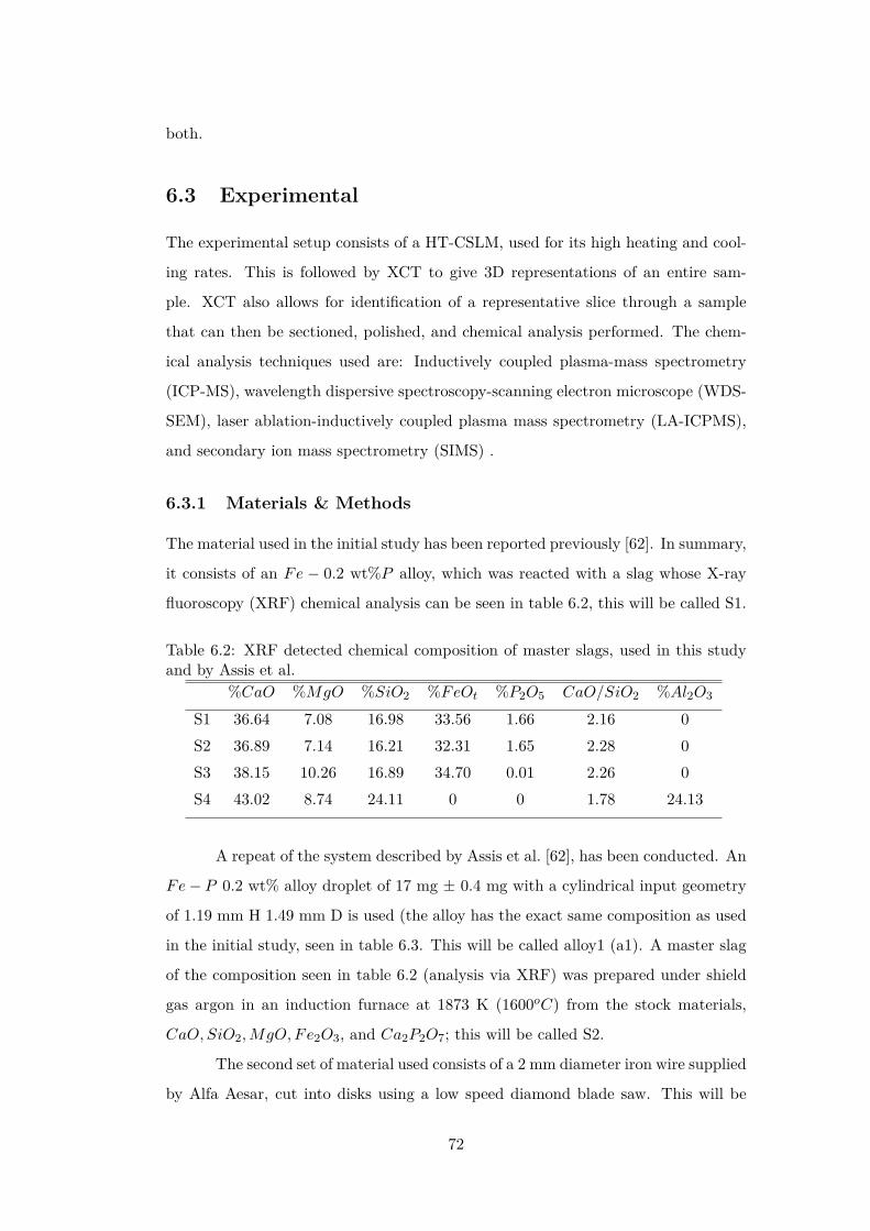
both.

6.3 Experimental

The experimental setup consists of a HT-CSLM, used for its high heating and cool-

ing rates. This is followed by XCT to give 3D representations of an entire sam-

ple. XCT also allows for identification of a representative slice through a sample

that can then be sectioned, polished, and chemical analysis performed. The chem-

ical analysis techniques used are: Inductively coupled plasma-mass spectrometry

(ICP-MS), wavelength dispersive spectroscopy-scanning electron microscope (WDS-

SEM), laser ablation-inductively coupled plasma mass spectrometry (LA-ICPMS),

and secondary ion mass spectrometry (SIMS) .

6.3.1 Materials & Methods

The material used in the initial study has been reported previously [62]. In summary,

it consists of an Fe − 0.2 wt%P alloy, which was reacted with a slag whose X-ray

fluoroscopy (XRF) chemical analysis can be seen in table 6.2, this will be called S1.

Table 6.2: XRF detected chemical composition of master slags, used in this studyand by Assis et al.

%CaO %MgO %SiO2 %FeOt %P2O5 CaO/SiO2 %Al2O3

S1 36.64 7.08 16.98 33.56 1.66 2.16 0S2 36.89 7.14 16.21 32.31 1.65 2.28 0S3 38.15 10.26 16.89 34.70 0.01 2.26 0S4 43.02 8.74 24.11 0 0 1.78 24.13

A repeat of the system described by Assis et al. [62], has been conducted. An

Fe− P 0.2 wt% alloy droplet of 17 mg ± 0.4 mg with a cylindrical input geometry

of 1.19 mm H 1.49 mm D is used (the alloy has the exact same composition as used

in the initial study, seen in table 6.3. This will be called alloy1 (a1). A master slag

of the composition seen in table 6.2 (analysis via XRF) was prepared under shield

gas argon in an induction furnace at 1873 K (1600oC) from the stock materials,

CaO, SiO2,MgO, Fe2O3, and Ca2P2O7; this will be called S2.

The second set of material used consists of a 2 mm diameter iron wire supplied

by Alfa Aesar, cut into disks using a low speed diamond blade saw. This will be

72

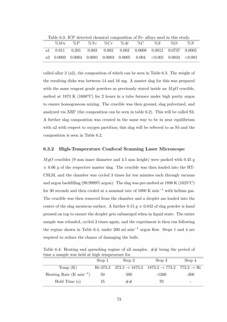
Table 6.3: ICP detected chemical composition of Fe- alloys used in this study.%Mn %P %Ni %Cr %Al %C %S %O %N

a1 0.011 0.201 0.003 0.002 0.002 0.0008 0.0012 0.0737 0.0005a2 0.0003 0.0004 0.0001 0.0003 0.0005 0.004 <0.001 0.0034 <0.001

called alloy 2 (a2), the composition of which can be seen in Table 6.3. The weight of

the resulting disks was between 14 and 16 mg. A master slag for this was prepared

with the same reagent grade powders as previously stated inside an MgO crucible,

melted at 1873 K (1600oC) for 2 hours in a tube furnace under high purity argon

to ensure homogeneous mixing. The crucible was then ground, slag pulverized, and

analyzed via XRF (the composition can be seen in table 6.2). This will be called S3.

A further slag composition was created in the same way to be in near equilibrium

with a2 with respect to oxygen partition; this slag will be referred to as S4 and the

composition is seen in Table 6.2.

6.3.2 High-Temperature Confocal Scanning Laser Microscope

MgO crucibles (9 mm inner diameter and 4.5 mm height) were packed with 0.45 g

± 0.06 g of the respective master slag. The crucible was then loaded into the HT-

CSLM, and the chamber was cycled 3 times for ten minutes each through vacuum

and argon backfilling (99.9999% argon). The slag was pre-melted at 1898 K (1625oC)

for 30 seconds and then cooled at a nominal rate of 1000 K min−1 with helium gas.

The crucible was then removed from the chamber and a droplet ass loaded into the

centre of the slag meniscus surface. A further 0.15 g ± 0.042 of slag powder is hand

pressed on top to ensure the droplet gets submerged when in liquid state. The entire

sample was reloaded, cycled 3 times again, and the experiment is then run following

the regime shown in Table 6.4, under 200 ml min−1 argon flow. Steps 1 and 4 are

required to reduce the chance of damaging the bulb.

Table 6.4: Heating and quenching regime of all samples. ## being the period oftime a sample was held at high temperature for.

Step 1 Step 2 Step 3 Step 4Temp (K) Rt-373.2 373.2 → 1873.2 1873.2 → 773.2 773.2 → Rt

Heating Rate (K min−1) 50 500 -1200 -300Hold Time (s) 45 ## 70 -

73

This was the same for all systems apart from that of S4, where a sapphire

crucible was used in order to increase scattered light detection, giving a way to

effectively increase the depth of focus field for the UV laser.

6.3.3 X-ray Computer Tomography

Samples containing S1 and S3, were scanned using a ‘Nikon Metrology XT H 320 LC’

XCT scanner and samples containing S2 and S4 were scanned using a ‘Zeiss Versa

520’. The difference in machines was due to the availability during experiments, with

the Zeiss preferred due to its better signal-to-noise ratio within images. This arises

from different source and detectors within the systems, and a smaller source/detector

distance in the Zeiss machine that is better suited for higher-resolution tomography.

The Nikon machine consists of a 225 kV micro focus with tungsten reflection

target and a flat panel detector consisting of 2000 x 2000 pixels, each of 200 microns

in size. The Zeiss machine has a 160 kV micro focus source with an alumina trans-

mission target and charge-couple device-based detector 2000 x 2000 pixels, with a

size dependant on the optic used (90.4 optic was used in this study with 1.75 micron

pixel size).

The parameters for each scan are shown in Table 6.5. The scans were then

reconstructed in proprietary packages included within the systems that use filtered

back projection. The reconstructed 3D volume was then evaluated in ‘VGStudio

MAX’ (Volume Graphics GmbH, Germany). Further information on the XCT

scanning including reference pieces used for scaling, determination of the droplet

isosurface, and validation of the scanning parameters can be found in previous

works [62] [81].

6.3.4 Chemical Analysis

In order to evaluate the phosphorus content in the metal before and during emulsifi-

cation for system 1 samples, WDS-SEM, LA-ICPMS, and SIMS were used. Each of

these techniques has the advantage of having small spot sizes which make it possible

to chemically analyse the metal drop and emulsion.

WDS-SEM was the initially selected tool to analyse the phosphorus content

in the metal drops as it is a non-destructive technique and relatively simple to use.

WDS offers better peak resolution and separation than EDS and can potentially

74

Table 6.5: Parameters used within the two scanners. ∗ There is an additionalfocusing step performed by an optic in the Zeiss machine, where x0.4 was usedin this study.

Nikon ZeissVoltage (kV) 220 140Power (W) 3.1 10Exposure 4 3

Projections 3142 3142Filter (mm) Cu 0.5 CaF2 1.0

Magnification x39.5 ∗x6.69Voxel Size 5.06 4.90

detect concentrations below 1 wt% with the usage of proper standards. Unlike

EDS, the detector reads and counts X-rays generated of a single wavelength at a

time that are diffracted by a crystal of proper lattice spacing. In the present study

the standards used were pure Fe and GaP for iron and phosphorus, respectively.

Each of the standards were used to standardize accelerating beam voltages of 25 and

30 kV with spot sizes of 6 and 7 microns. The high accelerating voltages and bigger

spot sizes were necessary in order to achieve the highest beam current possible in

the SEM, which helps in quantifying low concentrations.

LA-ICPMS differs from regular ICP-MS in that it uses a focused laser beam

to ablate a small area of the sample. This technique was used to confirm the data

acquired by WDS and only one sample was analysed via this technique. A total of

four measurements were taken using ICP-MS across different regions of the metal

drop. Each “shot” ablated roughly 5 µm in depth with a spot size of 100 µm in

diameter.

SIMS was used for the analysis of oxygen in the 20-second sample. SIMS

uses a focused ion beam to sputter the surface of the sample. As the ion beam mills

the surface, secondary ions are generated and these ions are analysed by a mass

spectrometer. Quantification was based on a stainless steel 302 standard.

6.4 Results and Discussion

The interaction of metal droplets with slag has been interrogated via the CT scan-

ning of quenched samples produced in the HT-CSLM. The first series reported by

75

Assis et al. [62], has now undergone initial chemical analysis of representative sec-

tioned surfaces (a1 and S1). Secondly a repeat of these initial conditions has been

completed to interrogate the consistency of the previously reported tomography re-

sults (a1 and S2), as well as further samples taken in the period before emulsification

to give insight into the pathway of the droplet breakup. Thus these experiments are

very similar and both will be referred to as system 1. As a result of the initial chem-

ical analysis of system 1, a low phosphorus system has been created and analysed

to investigate the true cause of emulsification (a2 and S3, system 2) in the previous

works. Finally a system at near equilibrium has been inspected via in situ imaging

in the CSLM (a2 and S4, system 3).

6.4.1 The Pathways of Emulsification

XCT scans of quenched samples for a system (system 1) have been reconstructed to

produce images seen in figure 6.1. It can be seen from figure 6.1 that emulsification

of the droplet in S2 has occurred.

Several points should be taken from these initial images that display signifi-

cant differences from the original study. Firstly, the holding times of these samples

cross over, and extend beyond that of the originals (0 to 120 seconds). This is most

likely because the repeat samples were run on a different HT-CSLM by a different

user; this resulted in a diverted regime, where it was found that the droplet was

taking longer to melt than seen before. At 90 seconds the sample is molten with

a spherical geometry and the surface can be seen to have begun to roughen, either

through the starting of initial emulsification, or due to the shrinkage of the droplet

in an uneven manner during quenching.

The next observation is the pathway of emulsification to coalescence is seen

to differ significantly from previously reported. This is thought to be due to the

slower heating rates seen within the new samples. A slower heating rate will have

caused slag and metal to become molten at a greater time separation. This will

potentially reduce the initial driving force of partition equilibration, as material will

begin to exchange before the droplet is fully molten. Due to this slower heating

rate and the need to hold material at high temperature for longer periods of time,

the amount of droplet dissolved into the slag could greatly increase. There are two

proposed pathways for the new samples in system 1:

76

Figure 6.1: Reconstructed images from XCT scanning, showing only the metal frac-tion of the sample

1. The droplet reaches molten state slowly, with initial refining taking place (90

seconds), emulsification begins with half the droplet breaking away (95 sec-

onds), the remaining sample continues to emulsify (140 seconds), and then

coalesces (155 seconds). Finally the sample continues to be dissolved into the

slag, reducing the visible material (170 seconds).

77

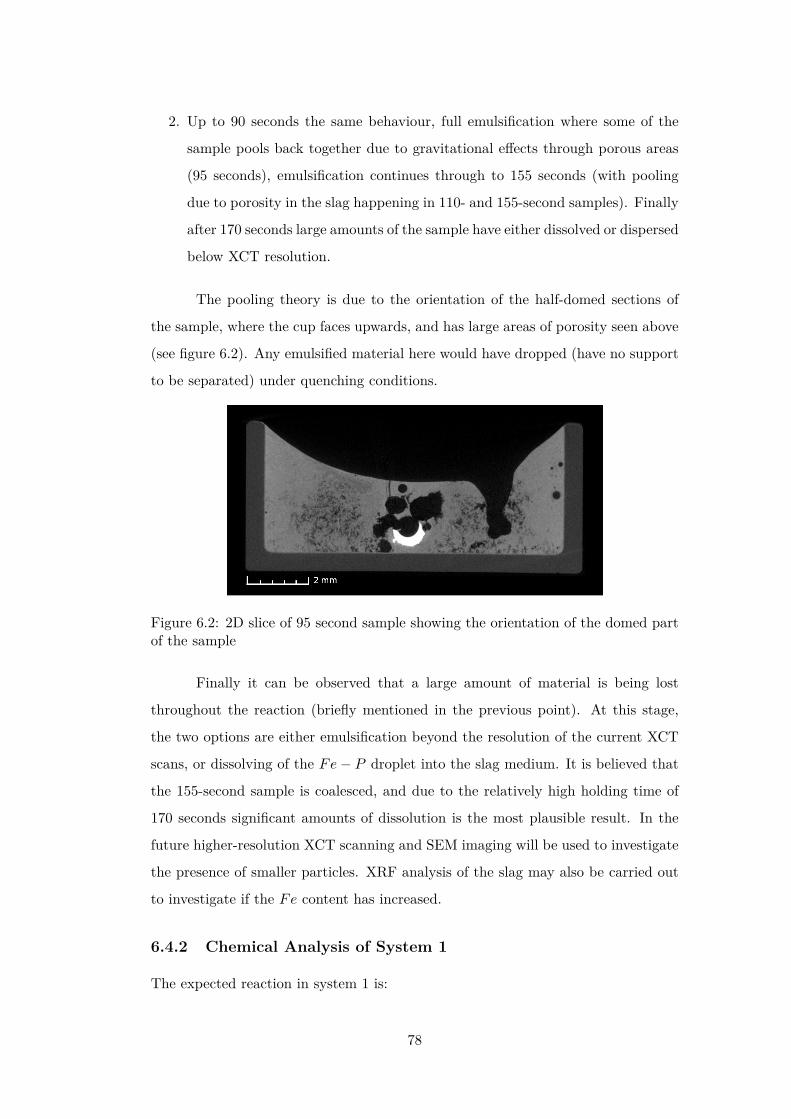
2. Up to 90 seconds the same behaviour, full emulsification where some of the

sample pools back together due to gravitational effects through porous areas

(95 seconds), emulsification continues through to 155 seconds (with pooling

due to porosity in the slag happening in 110- and 155-second samples). Finally

after 170 seconds large amounts of the sample have either dissolved or dispersed

below XCT resolution.

The pooling theory is due to the orientation of the half-domed sections of

the sample, where the cup faces upwards, and has large areas of porosity seen above

(see figure 6.2). Any emulsified material here would have dropped (have no support

to be separated) under quenching conditions.

Figure 6.2: 2D slice of 95 second sample showing the orientation of the domed partof the sample

Finally it can be observed that a large amount of material is being lost

throughout the reaction (briefly mentioned in the previous point). At this stage,

the two options are either emulsification beyond the resolution of the current XCT

scans, or dissolving of the Fe− P droplet into the slag medium. It is believed that

the 155-second sample is coalesced, and due to the relatively high holding time of

170 seconds significant amounts of dissolution is the most plausible result. In the

future higher-resolution XCT scanning and SEM imaging will be used to investigate

the presence of smaller particles. XRF analysis of the slag may also be carried out

to investigate if the Fe content has increased.

6.4.2 Chemical Analysis of System 1

The expected reaction in system 1 is:

78

5(FeO) + 2[P ]→ (P2O5) + 5[Fe] (6.1)

where the material in () is in the slag, and those in [] are in the metal droplet.

As previously mentioned WDS-SEM and LA-ICPMS were used for phospho-

rus analysis while SIMS was used for oxygen analysis. A total of 5 shots were made

close to the centre of the metal drop. Each shot milled roughly 10 µm in depth with

a spot size of 30 µm. A sixth oxygen measurement was performed using SIMS to

generate a depth profile of the oxygen concentration. This profile was obtained by

milling from the centre of the cross section of the droplet towards the interface of

the droplet. This profile is shown in figure 6.3. The summary of chemical analysis

carried out by each technique is shown in table 6.6.

Figure 6.3: Measured oxygen concentration as a function of depth into the 20ssample (using a cross section) from Assis et al [62]

Table 6.6: Summary of chemical analysis performed using the various techniquesdescribed

(wt.% P) (wt.% O)Reaction Time (s) ICP-MS WDS-SEM LA-ICPMS LECO SIMS

Original alloy 0.201 0.170±0.032 - 0.07370 - 0.179±0.015 - - -10 - 0.002±0.002 - - -20 - 0.008±0.005 0.0019±0.0001 - 0.213±0.13930 - 0.003±0.002 - - -

79

The results mapped against the previously reported surface area profiles of

the samples (Ai/A0) show that phosphorus had been removed from the droplet

before 10 seconds of reaction time (see figure 6.4). This was much sooner than

the first visualization of emulsification in system 1, at 30 seconds. This leads to

the conclusion that phosphorus exchange across the interface is not the reason for

emulsification to occur, and the equilibration time for phosphorus between metal

and slag is much shorter than the ideal predicted time of 120 seconds calculated

previously [62].

Figure 6.4: Expected oxygen concentration profile as a function of reaction time(LA-ICPMS only available at 20s)

SIMS results show a large increase in oxygen concentration within the droplet

at 20 seconds, as compared to the initial alloy (whose oxygen analysis was outsourced

to LECO). The Fe − FeO equilibrium based on the activity of FeO in the master

slag has been predicted using FactSage, giving oxygen equilibrium content within

the metal of ∼1000 ppm. This coupled with the calculated reduction in oxygen

early on due to reaction with phosphorus gives the predicted oxygen content as a

function of time mapped in figure 6.4. SIMS analysis showed an average oxygen

content of 0.213 ± 0.139 wt%, significantly higher than the predicted equilibrium.

Figure 6.3 also shows the heterogeneous distribution of oxygen radially through the

droplet, with values from below equilibrium to those much higher. SIMS does not

offer quantified data, however it should be within a factor of 2 when appropriate

standards are used.

80

From the points mentioned above, it is hypothesized that the exchange of

oxygen across the metal/slag interface is the cause of emulsification. It is not known

what would cause the mass oversaturation of oxygen within the droplet, however the

mass transfer of oxygen back into the slag to reach equilibrium between 20 and 30

seconds, would be rapid. This along with the known fact that oxygen is a surfactant

in a metal/slag system, leads the authors to the presented hypothesis.

In addition to the material presented, it was found that the cross-sectioned 0-

second sample contained a dispersion of particles throughout the droplet (see figure

6.5). Local WDS of these particles showed them to be significantly higher in phos-

phorus than the bulk material (from 1.7 to 3.1 wt% P ). These particles were not

seen in the cross-sectioned images of later samples, where the phosphorus levels were

seen to be drastically reduced (10 seconds onwards). Several images of the particles

were used to calculate an area fraction of 0.4%; with this and the average particle

concentration the amount of phosphorus removed is still significantly greater. It

is possible that the phosphorus was held in a phase which was immiscible or did

not melt at the same stage as the main bulk droplet; if this was the case, the high

phosphorus phase may have been removed on the macro scale through particle mi-

gration from the bulk liquid to the droplet surface. Thus mechanical features rather

than chemical reaction would be responsible for phosphorus removal. However, the

challenges associated with the chemical analysis of oxygen and phosphorous need to

be overcome before we can confirm whether the two reactions indeed can be sepa-

rated. This requires further interrogation in order to define a realistic mechanism

for phosphorus removal.

Figure 6.5: Low magnification SEM picture of ’P -rich’ particles

81

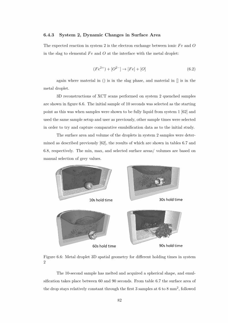
6.4.3 System 2, Dynamic Changes in Surface Area

The expected reaction in system 2 is the electron exchange between ionic Fe and O

in the slag to elemental Fe and O at the interface with the metal droplet:

(Fe2+) + [O2−]→ [Fe] + [O] (6.2)

again where material in () is in the slag phase, and material in [] is in the

metal droplet.

3D reconstructions of XCT scans performed on system 2 quenched samples

are shown in figure 6.6. The initial sample of 10 seconds was selected as the starting

point as this was when samples were shown to be fully liquid from system 1 [62] and

used the same sample setup and user as previously, other sample times were selected

in order to try and capture comparative emulsification data as to the initial study.

The surface area and volume of the droplets in system 2 samples were deter-

mined as described previously [62], the results of which are shown in tables 6.7 and

6.8, respectively. The min, max, and selected surface areas/ volumes are based on

manual selection of grey values.

Figure 6.6: Metal droplet 3D spatial geometry for different holding times in system2

The 10-second sample has melted and acquired a spherical shape, and emul-

sification takes place between 60 and 90 seconds. From table 6.7 the surface area of

the drop stays relatively constant through the first 3 samples at 6 to 8 mm2, followed

82

Table 6.7: Raw data for surface area measurements of system 3.Time (s) Surface Area Se-

lected (mm2)Surface Area Max(mm2)

Surface AreaMin(mm2)

Ai/A0

10 6.60 6.60 N.A 1.0030 8.37 8.38 8.36 1.2760 6.84 6.86 6.83 1.0490 65.75 73.69 58.13 9.96

Table 6.8: Raw data for volume measurements of system 2.Time (s) Volume

Selected(mm3)

VolumeMax (mm3)

VolumeMin (mm3)

Vi/V0

10 1.29 1.30 1.28 130 1.31 1.32 1.30 1.0260 1.19 1.19 1.18 0.9290 0.96 1.10 0.83 0.74

by an increase by an order of magnitude to 65.75 mm [47]. This increase in area

is very similar to that seen in the previous study [62]; however there is a delay of

∼30 seconds. This is clearly seen in the normalized area curves displayed in Figure

6.7. In system 2, oxygen is transferred from the slag into the metal, and the result

appears to validate the hypothesis of oxygen transfer across the interface being re-

sponsible for the spontaneous emulsification (the behaviour should occur regardless

of oxygen transfer direction). The delay of 30 seconds, may be a product of the fact

that no phosphorus exchange occurs in comparison to system 1, however it may also

be due to aspects such as inconsistent heat transfer inside the HT-CSLM, or other

parameters that affected the differences seen in system 2.

6.4.4 System 3, Validation of Chemical Exchange Causing Sponta-

neous Emulsification

A system designed with near equilibrium elemental distribution between slag and

metal phases has been used to validate the hypothesis of chemical exchange across

the interface being the cause of spontaneous emulsification.

System 3, notably has very low oxygen presence in the droplet (34 ppm)

and zero FeO/SiO2 in the slag phase (oxidation of Fe is thermodynamically un-

83

Figure 6.7: Normalized surface area of metal droplets as a function of time, for sys-tem 2 where oxygen from the slag enters the droplet, and system 1 where phosphorusfrom the droplet is being refined to the slag

favourable compared to all slag components).

It is known that thermal gradients across a medium can be a cause for spon-

taneous emulsification [60], and with the hot spot of the CSLM being ∼2 mm in

diameter (smaller than the sample), and heat transfer being required from sample

surface through the sample, it is unlikely the entire sample is constantly at the same

temperature, especially during heating and during the early period of the programed

isotherm.

System 3 being transparent in nature allowed for the in situ viewing of the

droplet throughout a reaction profile. It was seen that the droplet appears to stay

spherical in shape throughout the period of viewing, well past the previously reported

emulsification times. Figure 6.8 also shows an XCT cross section of the entire

sample, where the droplet is shown to be completely spherical and no Fe material was

detected separate from the main mass of iron. This sample had a smoother surface

than all previously reported samples not emulsified. The authors feel confident as a

result that thermal gradients are not the cause of emulsification in this case.

6.4.5 Mechanisms of Oxygen Transfer into the Droplet

Due to the highly basic nature of the slags used in this study, it is likely a bi-layer

would form at the interface with a cation and anion layering [99]. With this in mind,

it is possible that a stabilizing interaction forms as the ions order into a favourable

84

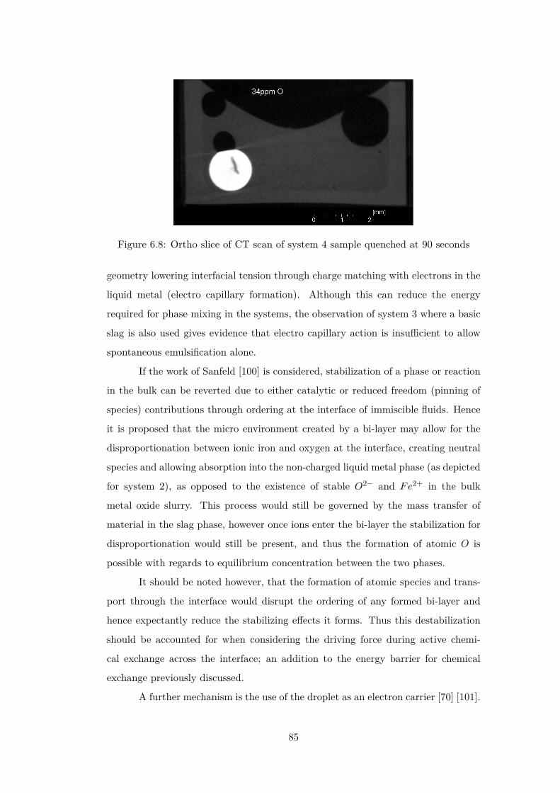
Figure 6.8: Ortho slice of CT scan of system 4 sample quenched at 90 seconds

geometry lowering interfacial tension through charge matching with electrons in the

liquid metal (electro capillary formation). Although this can reduce the energy

required for phase mixing in the systems, the observation of system 3 where a basic

slag is also used gives evidence that electro capillary action is insufficient to allow

spontaneous emulsification alone.

If the work of Sanfeld [100] is considered, stabilization of a phase or reaction

in the bulk can be reverted due to either catalytic or reduced freedom (pinning of

species) contributions through ordering at the interface of immiscible fluids. Hence

it is proposed that the micro environment created by a bi-layer may allow for the

disproportionation between ionic iron and oxygen at the interface, creating neutral

species and allowing absorption into the non-charged liquid metal phase (as depicted

for system 2), as opposed to the existence of stable O2− and Fe2+ in the bulk

metal oxide slurry. This process would still be governed by the mass transfer of

material in the slag phase, however once ions enter the bi-layer the stabilization for

disproportionation would still be present, and thus the formation of atomic O is

possible with regards to equilibrium concentration between the two phases.

It should be noted however, that the formation of atomic species and trans-

port through the interface would disrupt the ordering of any formed bi-layer and

hence expectantly reduce the stabilizing effects it forms. Thus this destabilization

should be accounted for when considering the driving force during active chemi-

cal exchange across the interface; an addition to the energy barrier for chemical

exchange previously discussed.

A further mechanism is the use of the droplet as an electron carrier [70] [101].

85

If we account for mass transport of Fe2+ in the slag to be the rate-limiting step, a

depletion of this ion at the surface is likely. As a result the reaction mechanism may

take advantage of the metal droplet reach through the slag (through not only its

large size compared to that of chemical interaction, but also the continued growth of

perturbations penetrating new areas of bulk slag) and the fast transport of electrons

through the liquid metal to reduce the kinetic constraints on oxygen uptake. The

steps for this mechanism are as follows:

1. Anionic oxygen transport across the interface from slag into the droplet

2. Transport of electrons through the metal droplet to a site in contact with an

iron cation

3. Transfer of the electrons to the iron cation to form an iron atom

4. Uptake of the neutral iron atom into the droplet

These steps can be expressed by the redox reactions:

(O2−)→ [O][2e−] (6.3)

(Fe2+) + [2e−]→ [Fe] (6.4)

where species in () are in the slag phase, and those in [] are in the metal

phase. Where O2− may be representative of a single oxygen ion or any reacting

complex containing the ion.

This mechanism requires the movement of a charged oxygen ion into the

non-charged metal droplet; this has a reliably large energetic cost and thus the

concentration gradient is required to be large in order for this to happen at any

meaningful rate. As such, this process may have a large influence early on in the

experiment, however as the process continues it is unlikely that this mechanism

could be responsible for the over saturation of oxygen seen from the SIMS results.

To interrogate these effects further, the authors propose experimentation

with lower basicity slags, and electrochemical experimentation. By these methods

it may be possible to isolate each effect and give quantification to its participation

in the phenomena reported here.

86

6.5 Conclusions and Revisiting the Hypothesis

Chemical analysis of samples from a previous study by Assis et al. [62] appear to

show that phosphorus movement across the interface between a metal drop and

slag is not responsible for spontaneous emulsification. Instead it is proposed that

oxygen partition in either direction across the interface causes a drop in interfacial

tension through surfactant effects and active refining. This is supported by a system

where only oxygen content was drastically away from equilibrium, showing similar

behaviour to that seen previously (apart from a slight delay). This statement directly

supports the interrogated hypothesis 3.

A replication of the previous study has also been carried out by another

user with a different HT-CSLM. This showed very different melting times for the

metal droplet and as a result a changed pathway of droplet morphology through the

reaction period. Discussion has been given as to why these differences may have

been seen, with heating performance, and sample preparation being the clearest

possibilities. It has also been seen that prior to emulsification the droplet appears

to show substantial roughening over the entire surface of the droplet, a link to the

emulsification mechanism.

Although the availability of oxygen is integral to the phosphorus refining to

the slag phase, the phosphorus appears to have completely equilibrated before emul-

sification occurs . This has however been potentially caused by a macroscopic flota-

tion effect of phosphorus rich phases not entering the liquid matrix of the droplet.

Hypothesis 4 requires further interrogation with a starting high phosphorus alloy

where the phosphorus is within the bulk matrix.

With the cause of spontaneous emulsification now justified, the pathway by

which this driving force causes emulsification must be considered. With a such study

there presents a possibility to predict spontaneous emulsification.

87

Chapter 7

Quantifying the Pathway and

Predicting Spontaneous

Emulsification During Material

Exchange in a Two Phase Liquid

System


Hypothesis 5: “Spontaneous emulsification is initiated by perturbation and the po-

tential this creates for reducing diffusion distance.”

Hypothesis 6: “Spontaneous emulsification can be predicted from fundamen-

tal knowledge of the system.”

With the knowledge as to why spontaneous emulsification occurs, the hy-

potheses above are presented to structure the interrogation of the emulsification

physical pathway and present a method to model the behaviour.

7.2 Introduction

Reaction rates dependent on the interfacial area between two phases is an encom-

passing multidisciplinary expanse of study. The problem approach is imperative, as

88

when diffusion in the bulk is rate limiting, the reduction in diffusion length offered

by mixing of systems can drastically speed up the rate of a reaction. This results in

higher efficiency and, if the necessary magnitude of change occurs, a different rate

limiting step. This can often manifest as spontaneous emulsification (SE) [60] [102]

of the species to form momentarily stabilized micro pockets of one phase dispersed

through the other [62] [103]. Considering this, it is desirable to create a system with

low interfacial tension, to allow the maximum sustained interfacial area. This can

be aided or stabilized [104] through several mechanisms: bi-layer formation, induced

charge gradients, surfactant addition and material exchange [86] [105] [27] [106].

In addition to classical areas [107] [108] [109] where interfacial breakdown is

sought to reduce or remove a kinetic barrier or naturally occurring high-temperature

reactions in geochemical systems, known systems where SE occurs can be utilized

to produce desirable micro dispersions instead of traditional physical shear methods

[58]. For example in silicon particle production [110], controlling the morphology of

polymeric membranes [31] and even the formation of edible systems for controlled

taste without affecting texture [111].

Mapping the transient interfacial area is key to understanding the rate of ma-

terial exchange between two immiscible liquids, as well as controlling and predicting

the phenomena such as the “tears of wine” or soap-aided spreading between hydro-

carbons and water [59]. These are prime examples of how interfaces can behave in

the presence of surface active species and physical influences causing a favourable

increase in immiscible phase contact area. The authors hypothesise that the manifes-

tations of these physical phenomena are controlled through the systematic growth,

necking and finally budding (when SE is considered) of perturbations at the liquid-

liquid interface. This cycle follows strict geometries controlled by the fundamental

properties of the species such that the resultant geometries can be understood and

predicted mathematically.

Here two systems are explored where the interfacial exchange of material

is thermodynamically favourable and very fast in comparison to the mass trans-

port of material in their bulk phases [67]. This situation is unusual in the lower

temperature systems home to classical interface studies, where the reaction at the

interface is often rate limiting. The systems being investigated consist of two im-

miscible phases, a molten metal and a molten oxide. Such systems are critical for

89

extraction refining, casting and welding of metallic alloys. System 1 consists of a

high-purity iron droplet and a high level of iron(ll) oxide in the molten oxide phase

(Fe − FeO system) to allow for quantification of the interface at varying stages of

emulsification. The active reaction within this system is displayed in equation 7.1,

and is of practical importance in the conversion of iron to steel during integrated

steel manufacturing. System 2 uses a high-aluminium alloyed iron droplet and an

enriched silicon dioxide oxide phase (FeAl−SiO2 system) for in-situ observation of

the emulsification’s physical pathway. The active reaction is shown in equation 7.2.

The latter is relevant for processing of low-density advanced high-strength steels for

automotive components, but also has the convenience of study in the present discus-

sion due to lack of transition metals in the oxide phase, making this phase optically

transparent.

(FeO)→ [Fe] + [O] (7.1)

4[Al] + 3(SiO2)→ 3[Si] + 2(Al2O3) (7.2)

where species in [] are present in the liquid metal phase, and those in () are within

the slag phase.

The findings from these experiments and further input from the literature

have been used to create a phase-field representation of the systems, where emul-

sification behaviour can be tracked and predicted through both chemical gradient

mapping and graphical representation of the interface morphology. It is suggested

while the reaction is occurring in these systems there is a chance the interface be-

tween the two phases perturbs. In addition, depending on the interfacial tension

chemical driving force the system may break up into an emulsion to facilitate the

faster dissipation of free energy.

7.3 Experimental

7.3.1 Materials

All molten oxide mixtures were prepared through powder mixing of reagent grade:

CaO, MgO, SiO2, Al2O3, CaO.P2O5, and FeO followed by pre-melting at 1873 K

90

for 2 hours in a horizontal tube furnace with use of either MgO (Fe−FeO system)

or Al2O3 crucibles (FeAl − SiO2 and null system). FeO was prepared through

heating of Fe2O3 and Fe at 1273 K for 4 hours in a F e crucible using a 99.9999%

Ar environment (used for the mixture pre-melts as well). After pre-melting the oxide

mixtures were then ground using a disk mill. Molten oxide mixture compositions

were measured using XRF.

Samples containing the iron alloy of composition 0.0003% Mn, 0.0004% P ,

0.0001% Ni, 0.0003% Cr, 0.0005% Al, 0.004% C, 0.001% S, 0.0034% O, <0.001

N , and slag of composition 36.89% CaO, 7.14% MgO, 16.21% SiO2, 32.31% FeOt,

1.65% P2O5, comprise the Fe − FeO system. Experiments were conducted using

high-density MgO crucibles.

Samples containing the iron alloy of the same composition as the Fe− FeO

system and slag with the composition 43.02% CaO, 8.74% MgO, 24.11% SiO2,

24.11% Al2O3 comprise the null experimental system. Experiments were conducted

using sapphire crucibles. Samples containing the iron alloy of composition 0.0002%

Mn, 0.0004% P , 0.002% Ni, 0.0005% Cr, 7.87% Al, 0.0007% C, 0.001% S, 0.0038%

O, <0.001% N and slag of composition 36.17% CaO, 23.11% SiO2, 38.53% Al2O3

comprise the FeAl − SiO2 system. Experiments were conducted using sapphire

crucibles.

7.3.2 High-Temperature Confocal Scanning Laser Microscopy

A scanning UV laser is then used to view the sample while the experiment is con-

ducted, recording at 15 fps with use of the HiTOS software package. A widening

aperture function (inbuilt within the machine) was also used on the laser focusing

to increase field of view in the z-direction (this reduces resolution in grey-scale ac-

curacy when analysing the recorded video, this is the reason no size quantification

is appropriate from the HT-CSLM images).

0.2 g ± 0.034 of molten oxide was loaded into a crucible. The mix was then

pre-melt using the HT-CSLM, following the same heating cycle as shown in figure

7.6 with the 0-second hold. After cooling a metal cylinder of dimensions 1.19 mm H,

1.49 mm D weighing 17 mg ± 0.52 is added into the centre of the quenched molten

oxide meniscus and a further 0.3g ± 0.12 of molten oxide is then added on top of

the cylinder. This is followed by lightly compressing the powder by hand before the

91

sample is loaded into the HT-CSLM for the experimental heating cycle. In the case

of the null experiment system and the FeAl − SiO2 system samples, a separate Pt

and Al2O3 spacer are added to the underside of the crucible. The platinum spacer is

used to increase reflected light through the sample, giving greater depth of vision in

the HT-CSLM. The alumina spacer is present to stop sticking of the Pt spacer to the

Pt sample holder. The chamber is evacuated using a rotary pump for 30 minutes and

back filled three times. Experiments are run under an inert atmosphere of 99.9999%

Ar passed through a further 623 K heated getter containing Cu and Mg chips.

Experimental times reported are normalized through determination of the

molten oxide entering a fully liquid state, as viewed through the HT-CSLM video

output. This time varied from between 5 and 25 seconds after reaching the pro-

grammed temperature of 1873 K. Reasons for this are expectedly due to variation in

HT-CSLM performance, chamber maintenance, as well as effective interaction with

the IR radiation due to differences in the sample surface topology (surface roughness

for example [112]) and powder packing density.

7.3.3 Micro X-ray Computer Tomography

The samples were scanned using a ‘Zeiss Versa 520’, which has a 160 kV micro focus

source with an alumina transmission target and charge-couple device-based detector

2000 x 2000 pixels, with a size dependent on the optic used. The machine has a

cone beam X-ray source and a rotating turntable between source and detector.

The scanning parameters used were: voltage 140 kV, power 10 W, exposure

3 s, projections 3142, filter CaF2 1.0 mm, magnification x6.69∗, voxel size 4.90. The

additional optical focusing used was x0.4.

The scans are then reconstructed in a proprietary package included within

the systems that use filtered back projection. The 3D volume is reconstructed using

a Feldkamp back projection method, creating a series of volume elements. The

3D volumes are then evaluated using ‘VGStudio MAX’ (Volume Graphics GmbH,

Germany).

The surface area and volume of the iron pellet is evaluated by individual

segmentation to determine the surface based on grey values, enabling selection of an

appropriate isosurface. To ensure consistency the selected isosurface was automati-

cally determined by the program through selection of sample voxels considered to be

92

background (air) and the material (iron). Strong contrast in grey values between the

oxide and metal fractions of the sample aided in the precise determination. Through

this mechanism all measurements will be subject only to a consistent error across

all samples.

To combat the inherent errors within XCT scanning (dependent on the given

detector-source/source-object distance) a precision ball bar with a centre-to-centre

distance of 5 mm is scanned. The results of the size evaluation of this can then be

used to rationalize that of the experimental samples. Further information on XCT

scanning parameter validation and development of the isosurface measurement can

be found in previous works [62] [81].

7.3.4 Phase-Field Modelling

A phase-field theory of liquid phase separation coupled to fluid flow is employed for

the current study. The respective Cahn-Hillard-type and Navier-Stokes equations

are solved numerically. The interfacial free energy is assumed to be γ = 60 mJ

m−2 [113]. The free energies of the bulk liquid phases are taken from the regular

solution model. During the simulation the temperature was fixed. The time scale

of the process is set by the interplay of melt flow and chemical diffusion [114] [115].

The equation of motion was made dimensionless using the length and time scale ζ =

6 x 10−6 cm, Γ = ζ2/D = 1.2 µ s, where D = 3 x 10−5 cm2 s−1 and is the diffusion

coefficient. The dimensionless time and spatial steps were chosen as ∆t = 1.25x10−7

and ∆x = 5x10−3.

7.4 Results and Discussion

In figure 7.1 a cross section of a quenched system at equilibrium (<34 ppm O2 Fe

droplet, with a slag containing no FeO) produced from X-ray Computed Tomogra-

phy (XCT), an almost perfectly spherical geometry is found. Figure 7.2 is a series of

stills taken from high-temperature confocal scanning laser microscopy (HT-CSLM)

of the equilibrium system over a period crossing the emulsification times of both

reactive systems. Very slight perturbation can be seen at times during the anal-

ysed recording, yet no individual wave shows sustained growth. Hazing and lack

of distinction in the images is expected as the HT-CSLM is able to view a narrow

93

vertical slice of an extremely dynamic 3D system, where the imaging light is also

undergoing refraction when exiting the molten surface. Both the appearance of the

spherical droplet identified through XCT scanning and the lasting placidity of the

droplet viewed in-situ, give a standard behaviour against which to set the rest of

our findings. The lack of emulsification shows temperature gradients and surfactant

stabilization are unable to cause SE by themselves within the systems explored [86].

XCT images presented in figure 7.3 show only the metal proportion (light grey)

of scanned samples produced from the Fe − FeO system. From left to right (in-

creasing in time after reaching 1873 K) a progression of emulsification is observed:

the droplet has formed into a molten sphere on reaching temperature; perturbation

begins on the droplet surface; the level of perturbation drastically increases and a

small amount of material is seen to have separated; a gradually increasing portion of

the droplet has entered a highly emulsified state (20-45 seconds); the entire sample

has broken down to form a fully emulsified droplet (65 seconds).

Figure 7.1: A 2D XCT reconstruction of a system at equilibrium, where the metaldroplet is displayed in white, the slag in light grey, the crucible in dark grey andporosity as black (3µm resolution scan).

94

Figure 7.2: A three step sequence showing the quiescent droplet in the equilibriumsystem with time as imaged by the HT-CSLM through a transparent slag.

95

0 s

eco

nd

s2

0 s

eco

nd

s2

5 s

eco

nd

s4

5 s

eco

nd

s6

5 s

eco

nd

s

350 µ

m

Figu

re7.

3:R

econ

stru

cted

XC

Tim

ages

ofth

eFe−FeO

syst

emqu

ench

edat

defin

edtim

es;o

nly

the

met

alpa

rtof

the

sam

ple

isdi

spla

yed

inlig

htgr

ey(3µ

mre

solu

tion

scan

).

96

Figure 7.4 offers a qualitative view of the level of perturbation change between

20 and 25 seconds. The images at the top show the 20-second sample having a

significantly higher area of the segmental perturbations in the darker blue end of

the scale spectrum, as opposed to the 25-second sample where the image depicts on

average a longer perturbation distance from the segmentation sphere and multiple

perturbations at the very top of the length scale, above 400 µm in length. As the

reaction progresses, perturbations grow due to sustained transfer of material between

slag and metal phase; the lowering of diffusion distances through growth allows for

the faster dissipation of free energy. The effect is an increase in perturbation size

and overall interfacial area increase; the energetic cost of increased interfacial area

must be outweighed by the free energy release [90]. The metallic material can be

envisaged as being dragged into the perturbation by the expanding surface. This is

quantified in figure 7.5 where the surface areas of the metal droplets from figure 7.3

are presented along with the expected change in surface area of the null experiment

previously discussed. Here it can be seen that the increased perturbation level

between the 20- and 25-second samples has resulted in a slight increase in surface

area. The null experiment shows a slight reduction in surface area due to loss of

material through oxidation and dissolution into the slag phase with time (modelled

using FactSageTM ). Examples of heating profiles entered in the HT-CSLM for the

experiments discussed are given in figure 7.6; the HT-CSLM was able to follow these

profiles to within ±10oC with the most deviation at the point of change between

heating to reaction temperature (1873 K) and the isotherm.

Next the FeAl − SiO2 system is considered, where in figure 7.7 a time-

step HT-CSLM image sequence is presented of the system during reaction at low

magnification. The droplet can be seen to increase in size followed by distortion

and observation of perturbations. The material then spreads into a cloud covering

most of the field of view before coalescence back to a near-spherical shape. Figure

7.8 shows the same reaction at higher magnification; the stage of SE can clearly be

observed: random perturbation beginning; growth in both size and number of these

perturbations; complete breakdown/clouding of the system over the entire image;

finally coalescence of the system to a single near-spherical shape. Due to the speed

of this reaction the droplet was unobservable from the very commencement of slag

melting, as such the first image of Figure 7.8 shows slight perturbation already. Only

97

20 seconds

25 seconds

Figure 7.4: 3D reconstructions of the 20- and 25-second samples, with the addition ofthe segmented perturbations displayed in colour dependent on length of protrusionfrom the segmentation sphere.

the last image shows a smooth droplet similar to those seen in the null experiment

which coincides with when the FeAl−SiO2 system should have reached equilibrium.

98

Figure 7.5: The quantified surface area of the metal droplet in the Fe−FeO systemwith time from XCT analysis, along with the expected surface area of the nullexperiment assuming a perfectly quiescent sphere; the null experiment surface areareduces with time due to slight oxidation as modelled using the equilibrium modulein FactsageTM .

Figure 7.6: The programmed heating cycle of the HT-CSLM, showing a slow earlyheating regime and a quench point on cooling for protection of the equipment againstthermal shock.

99

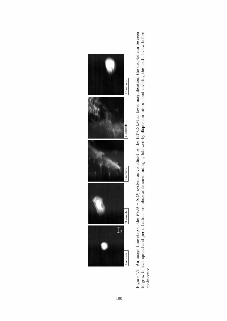
3 s

eco

nd

s2

0 s

eco

nd

s1

1 s

eco

nd

s9

sec

on

ds

0 s

eco

nd

s

1 m

m

Figu

re7.

7:A

nim

age

time

step

ofth

eFeAl−SiO

2sy

stem

asvi

sual

ised

byth

eH

T-C

SLM

atlo

wer

mag

nific

atio

n;th

edr

ople

tca

nbe

seen

togr

owin

size,

spre

adan

dpe

rtur

batio

nsar

eob

serv

able

surr

ound

ing

it,fo

llowe

dby

disp

ersio

nin

toa

clou

dco

verin

gth

efie

ldof

view

befo

reco

ales

cenc

e.

100

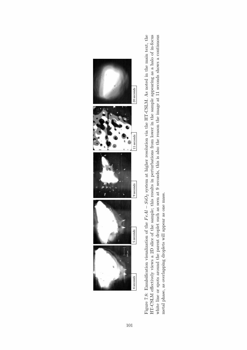
20

sec

on

ds

11

sec

on

ds

9 s

eco

nd

s5

sec

on

ds

4 s

eco

nd

s

300 µ

m

Figu

re7.

8:Em

ulsifi

catio

nvi

sual

izat

ion

ofth

eFeAl−SiO

2sy

stem

athi

gher

reso

lutio

nvi

ath

eH

T-C

SLM

.As

note

din

the

mai

nte

xt,t

heH

T-C

SLM

effec

tivel

yvi

ews

a2D

slice

ofth

esa

mpl

e;th

isre

sults

inpe

rtur

batio

nsfro

mlo

wer

inth

esa

mpl

eap

pear

ing

asa

halo

ofin

-focu

sw

hite

line

orsp

ots

arou

ndth

epa

rent

drop

let

such

asse

enat

9se

cond

s,th

isis

also

the

reas

onth

eim

age

at11

seco

nds

show

sa

cont

inuo

usm

etal

phas

e,as

over

lapp

ing

drop

lets

will

appe

aras

one

mas

s.

101

Quenched samples of the FeAl−SiO2 system are displayed in figure 7.9 where

the 15-second sample (the quickest time in which this sample could be captured with

reduced cooling performance due to the experimental setup of this system) can be

seen to have undergone significant coalescence. Yet there are still a large number of

well dispersed smaller droplets throughout the sample. The 20-, 25- and 30-second

samples show a reduced number and size of droplets outside the main coalesced body.

The surface area and detected volume of metal in these samples has been added in

figure 7.10, where it is clearly visible that the FeAl−SiO2 system is coalescing and

near complete equilibrium within the same time frame that the Fe − FeO system

begins emulsification to a significant extent. This shows significant differences in

the rate of reactive species mobility in the systems, where the Fe− FeO system is

most likely dependent on the rate of mass transport of FeO through the slag phase,

whereas the FeAl − SiO2 system is likely dependent on Al mass transport in the

metal phase [74] [75].

30 seconds

20 seconds

750 µm

15 seconds

25 seconds

Figure 7.9: 3D reconstructions of the quenched FeAl − SiO2 system where thecrucible and slag phases have been removed to expose the metal phase of the samplein free space.

The classical Fick’s law which is generally known for explaining the diffu-

102

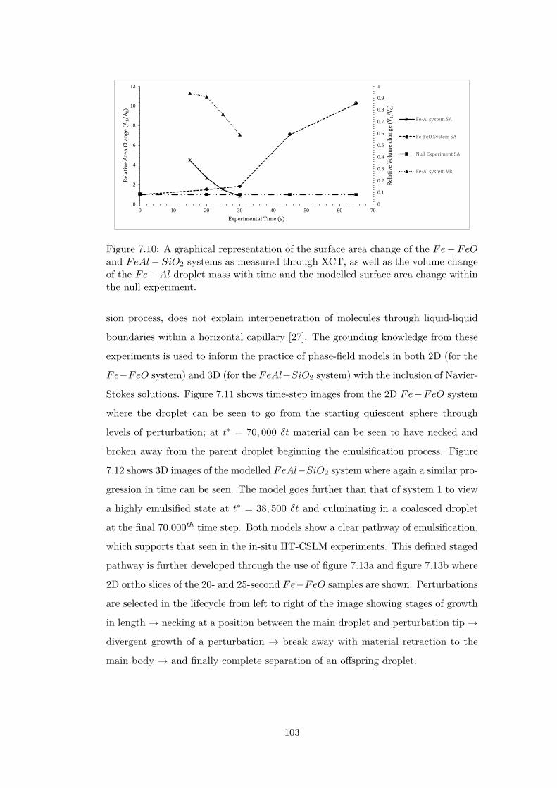
0

0.1

0.2

0.3

0.4

0.5

0.6

0.7

0.8

0.9

1

0

2

4

6

8

10

12

0 10 20 30 40 50 60 70

Rel

ativ

e V

olu

me

chan

ge (

V1/

V0)

Rel

ativ

e A

rea

Ch

ange

(A

1/

A0)

Experimental Time (s)

Fe-Al system SA

Fe-FeO System SA

Null Experiment SA

Fe-Al system VR

Figure 7.10: A graphical representation of the surface area change of the Fe−FeOand FeAl− SiO2 systems as measured through XCT, as well as the volume changeof the Fe−Al droplet mass with time and the modelled surface area change withinthe null experiment.

sion process, does not explain interpenetration of molecules through liquid-liquid

boundaries within a horizontal capillary [27]. The grounding knowledge from these

experiments is used to inform the practice of phase-field models in both 2D (for the

Fe−FeO system) and 3D (for the FeAl−SiO2 system) with the inclusion of Navier-

Stokes solutions. Figure 7.11 shows time-step images from the 2D Fe−FeO system

where the droplet can be seen to go from the starting quiescent sphere through

levels of perturbation; at t∗ = 70, 000 δt material can be seen to have necked and

broken away from the parent droplet beginning the emulsification process. Figure

7.12 shows 3D images of the modelled FeAl−SiO2 system where again a similar pro-

gression in time can be seen. The model goes further than that of system 1 to view

a highly emulsified state at t∗ = 38, 500 δt and culminating in a coalesced droplet

at the final 70,000th time step. Both models show a clear pathway of emulsification,

which supports that seen in the in-situ HT-CSLM experiments. This defined staged

pathway is further developed through the use of figure 7.13a and figure 7.13b where

2D ortho slices of the 20- and 25-second Fe−FeO samples are shown. Perturbations

are selected in the lifecycle from left to right of the image showing stages of growth

in length→ necking at a position between the main droplet and perturbation tip→

divergent growth of a perturbation → break away with material retraction to the

main body → and finally complete separation of an offspring droplet.

103

17

50

0 t

ime

step

s0

tim

e st

eps

35

00

0 t

ime

step

s7

00

00

tim

e st

eps

Figu

re7.

11:

Sele

cted

grap

hica

lout

puts

from

the

2DFe−FeO

phas

e-fie

ldm

odel

ling

show

ing

the

prog

ress

ion

from

aqu

iesc

ent

sphe

reto

ahi

ghly

pert

urbe

dst

ate

whe

rem

ater

ialh

asbe

gun

tobr

eak

away

from

the

pare

ntdr

ople

t.

104

17

50

0 t

ime

step

s0

tim

e st

eps

31

00

0 t

ime

step

s3

85

00

tim

e st

eps

70

00

0 t

ime

step

s

Figu

re7.

12:

3Dgr

aphi

calo

utpu

tsfro

mth

eFeAl−SiO

2ph

ase-

field

mod

el,w

here

the

full

life

cycl

eof

emul

sifica

tion

and

coal

esce

nce

can

bese

enw

ithin

the

simul

ated

70,0

00tim

est

eps.

105

Growing Necking Diverging Budding Full Separation

20 seconds 25 seconds

200 µm

a)

b)

Figure 7.13: a) 2D ortho slices of the XCT 20- and 25-second reconstructions wherethe metal phase is in light grey, slag in dark grey and porosity in black. b) Magnifiedsection of the 20- and 25-second ortho slice images where each growth cycle stage ofa perturbation as identified from the phase-field modelling has been highlighted aspresent in the experimental samples.

The similarity between the patterns of behaviour observed for perturbations

in both the experimental and modelling approach give strong validation of the mod-

els’ driving forces. Equally the time-step images from the 3D phase field model and

the in-situ HT-CSLM video of the same system can then be correlated. This offers

a method to deduce the number of time steps in the model equivalent to a period

of time in the high-temperature experiments. This results in 3,500 time steps being

equivalent to 1 second. In figure 7.14 the culmination of the two experimental sys-

tems’ interfacial area ratios where time has been converted to time steps is given,

as well as the addition of both the FeAl − SiO2 system and Fe − FeO system

interfacial area ratios computed from the phase-field model. From this it is clearly

observable that both pairings have a high level of coherency between the modelled

data and experimental measurement with several overlapping data points between

each. Although there is slight deviation, this is expected to be due to temperature

variation in the experimental method (under heating in the case of the Fe − FeO

system limiting diffusion rates, and cooling during the quenching of the FeAl−SiO2

106

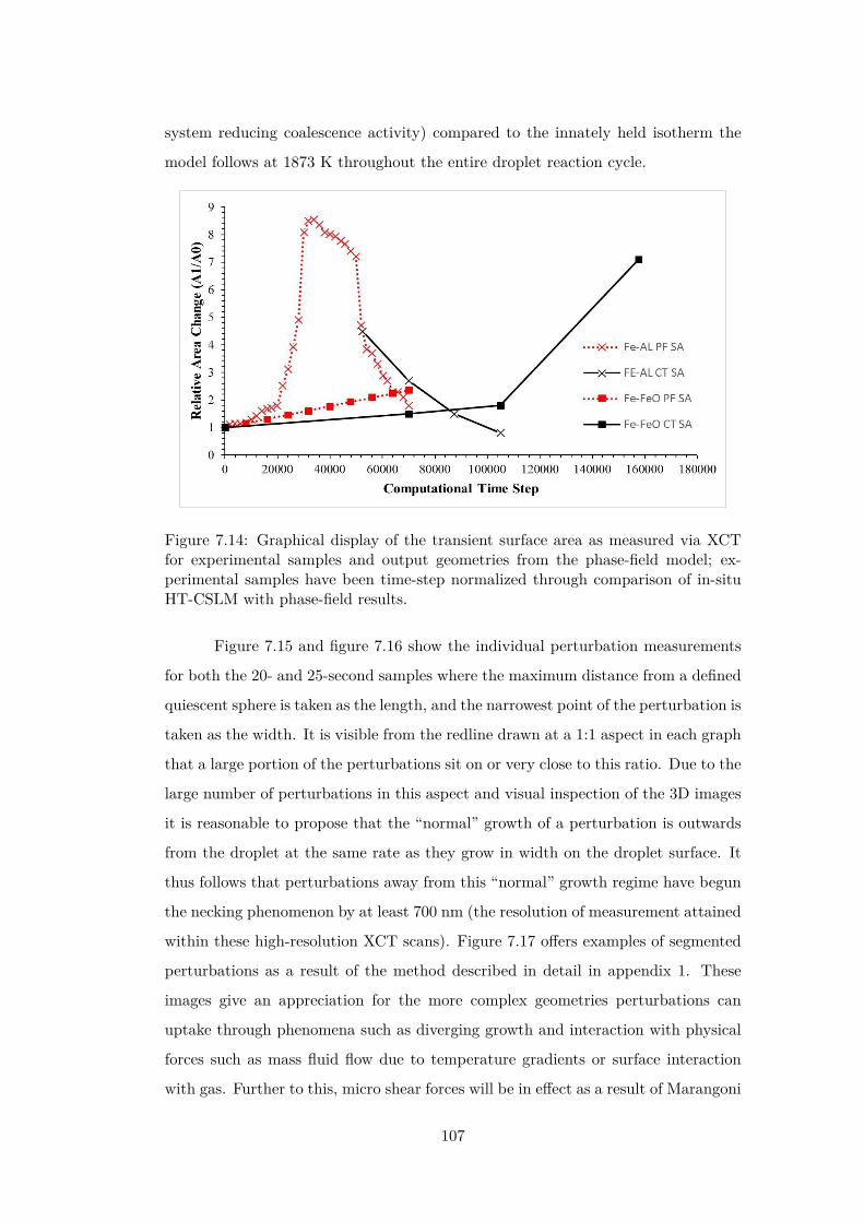
system reducing coalescence activity) compared to the innately held isotherm the

model follows at 1873 K throughout the entire droplet reaction cycle.

Figure 7.14: Graphical display of the transient surface area as measured via XCTfor experimental samples and output geometries from the phase-field model; ex-perimental samples have been time-step normalized through comparison of in-situHT-CSLM with phase-field results.

Figure 7.15 and figure 7.16 show the individual perturbation measurements

for both the 20- and 25-second samples where the maximum distance from a defined

quiescent sphere is taken as the length, and the narrowest point of the perturbation is

taken as the width. It is visible from the redline drawn at a 1:1 aspect in each graph

that a large portion of the perturbations sit on or very close to this ratio. Due to the

large number of perturbations in this aspect and visual inspection of the 3D images

it is reasonable to propose that the “normal” growth of a perturbation is outwards

from the droplet at the same rate as they grow in width on the droplet surface. It

thus follows that perturbations away from this “normal” growth regime have begun

the necking phenomenon by at least 700 nm (the resolution of measurement attained

within these high-resolution XCT scans). Figure 7.17 offers examples of segmented

perturbations as a result of the method described in detail in appendix 1. These

images give an appreciation for the more complex geometries perturbations can

uptake through phenomena such as diverging growth and interaction with physical

forces such as mass fluid flow due to temperature gradients or surface interaction

with gas. Further to this, micro shear forces will be in effect as a result of Marangoni

107

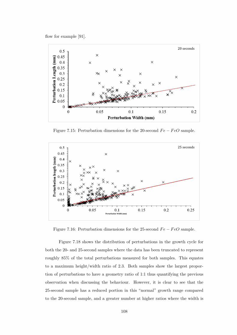
flow for example [91].

20 seconds

Figure 7.15: Perturbation dimensions for the 20-second Fe− FeO sample.

Perturbation Width (mm)

25 seconds

Figure 7.16: Perturbation dimensions for the 25-second Fe− FeO sample.

Figure 7.18 shows the distribution of perturbations in the growth cycle for

both the 20- and 25-second samples where the data has been truncated to represent

roughly 85% of the total perturbations measured for both samples. This equates

to a maximum height/width ratio of 2.3. Both samples show the largest propor-

tion of perturbations to have a geometry ratio of 1:1 thus quantifying the previous

observation when discussing the behaviour. However, it is clear to see that the

25-second sample has a reduced portion in this “normal” growth range compared

to the 20-second sample, and a greater number at higher ratios where the width is

108

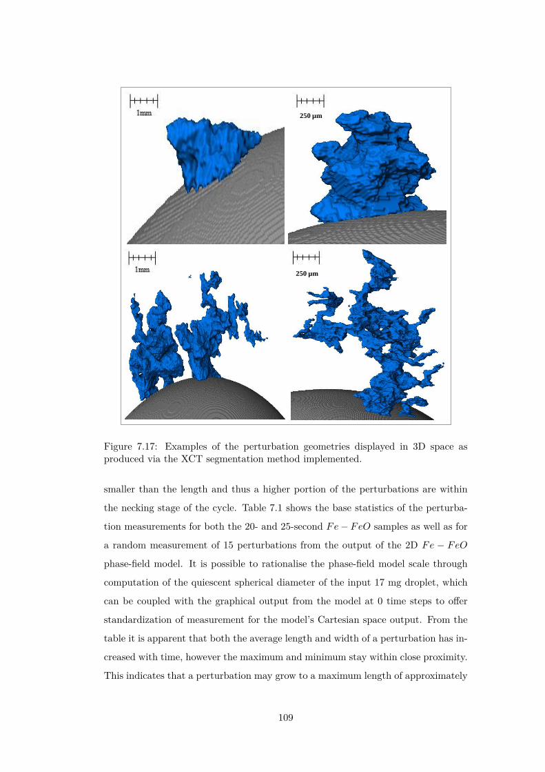
1mm 250 µm

250 µm

Figure 7.17: Examples of the perturbation geometries displayed in 3D space asproduced via the XCT segmentation method implemented.

smaller than the length and thus a higher portion of the perturbations are within

the necking stage of the cycle. Table 7.1 shows the base statistics of the perturba-

tion measurements for both the 20- and 25-second Fe− FeO samples as well as for

a random measurement of 15 perturbations from the output of the 2D Fe − FeO

phase-field model. It is possible to rationalise the phase-field model scale through

computation of the quiescent spherical diameter of the input 17 mg droplet, which

can be coupled with the graphical output from the model at 0 time steps to offer

standardization of measurement for the model’s Cartesian space output. From the

table it is apparent that both the average length and width of a perturbation has in-

creased with time, however the maximum and minimum stay within close proximity.

This indicates that a perturbation may grow to a maximum length of approximately

109

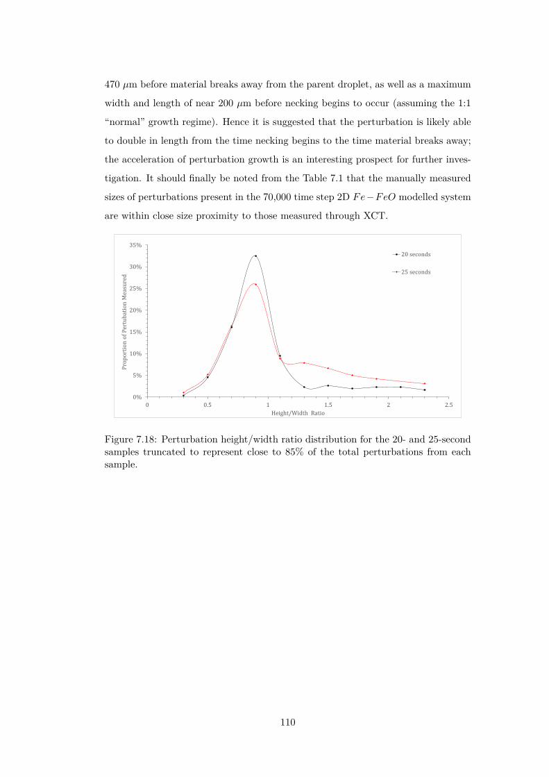
470 µm before material breaks away from the parent droplet, as well as a maximum

width and length of near 200 µm before necking begins to occur (assuming the 1:1

“normal” growth regime). Hence it is suggested that the perturbation is likely able

to double in length from the time necking begins to the time material breaks away;

the acceleration of perturbation growth is an interesting prospect for further inves-

tigation. It should finally be noted from the Table 7.1 that the manually measured

sizes of perturbations present in the 70,000 time step 2D Fe−FeO modelled system

are within close size proximity to those measured through XCT.

0%

5%

10%

15%

20%

25%

30%

35%

0 0.5 1 1.5 2 2.5

Pro

po

rtio

n o

f P

ertu

bat

ion

Mea

sure

d

Height/Width Ratio

20 seconds

25 seconds

Figure 7.18: Perturbation height/width ratio distribution for the 20- and 25-secondsamples truncated to represent close to 85% of the total perturbations from eachsample.

110

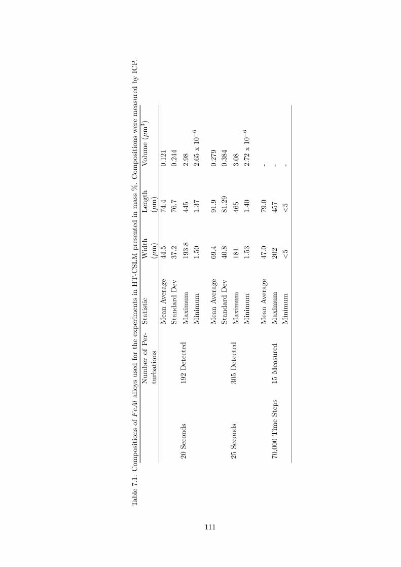
Tabl

e7.

1:C

ompo

sitio

nsofFeAl

allo

ysus

edfo

rth

eex

perim

ents

inH

T-C

SLM

pres

ente

din

mas

s%

.C

ompo

sitio

nswe

rem

easu

red

byIC

P.N

umbe

rof

Per-

turb

atio

nsSt

atist

icW

idth

(µm

)Le

ngth

(µm

)Vo

lum

e(µ

m3 )

Mea

nAv

erag

e44

.574

.40.

121

Stan

dard

Dev

37.2

76.7

0.24

420

Seco

nds

192

Det

ecte

dM

axim

um19

3.8

445

2.98

Min

imum

1.50

1.37

2.65

x10−

6

Mea

nAv

erag

e69

.491

.90.

279

Stan

dard

Dev

40.8

81.2

90.

384

25Se

cond

s30

5D

etec

ted

Max

imum

181

465

3.08

Min

imum

1.53

1.40

2.72

x10−

6

Mea

nAv

erag

e47

.079

.0-

70,0

00T

ime

Step

s15

Mea

sure

dM

axim

um20

245

7-

Min

imum

<5

<5

-

111

With validation of the phase-field model through physical interrogation of its

graphical expression as compared to the experimental observation and measurement,

the exploration of mapping both the physical force and chemical distribution in the

systems is possible. The dynamics of the 3D FeAl − SiO2 system with respect

to the stages of a perturbation’s growth and separation from the parent droplet

are possible to output from the model. Figure 7.19 maps the interfacial tension

between the two phases with respect to geographical location. The surface tension

is seen to be highest at the tip of the perturbation during growth, however when the

perturbation reaches a certain size this tension reduces due to reduced curvature.

At the same time a shift is visible of high surface tension to the necking area of the

droplet, which as the neck increases in length becomes high enough to cause release

of the budding section of the perturbation, relieving the highly constrained necking

area to lower the surface tension overall.

The aluminium level within the sample can be viewed as a profile of depth

into the metal droplet from the slag/metal interface, as well as in the perturbation

compared to the bulk droplet in Figure 7.20. The model predicts a reduction in

aluminium content radially outwards through the droplet, supportive of the mass

transfer of aluminium being the rate-controlling step in this system. The high surface

area to volume ratio within a perturbation presents a greater concentration gradient

in this area of the droplet, pulling more and more aluminium from the bulk droplet

into the perturbation. This is driven through the higher chemical gradient (faster

than it would approach the surrounding quiescent interface) creating a higher con-

centration of aluminium in the “bulk” perturbation than in the surrounding surface

of the droplet. Finally figure 7.21 shows the distribution of the normalized gradient

of driving force including the chemical free energy and the interfacial energy within

a drop. Although there is an increase in the number of reactive elements ejected

into the perturbation; due to the increased curvature at the necking area, there is a

larger gradient of driving force (similar to surface tension) in this area compared to

the peripheral of the drop where the curvature is less as a result of the differences

in the spacing between iso-concentration contours near the interface. After the sep-

aration, there is a uniform distribution of the gradient at the periphery areas of the

original drop and that of the separated droplet and both systems evolve towards

decreasing their interfacial energies (surface areas). This process continues until the

112

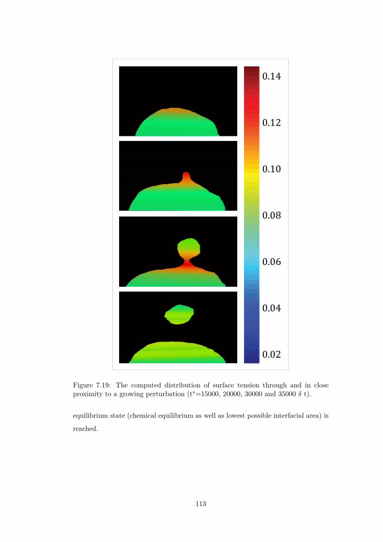
0.14

0.12

0.10

0.08

0.06

0.04

0.02

Figure 7.19: The computed distribution of surface tension through and in closeproximity to a growing perturbation (t∗=15000, 20000, 30000 and 35000 δ t).

equilibrium state (chemical equilibrium as well as lowest possible interfacial area) is

reached.

113

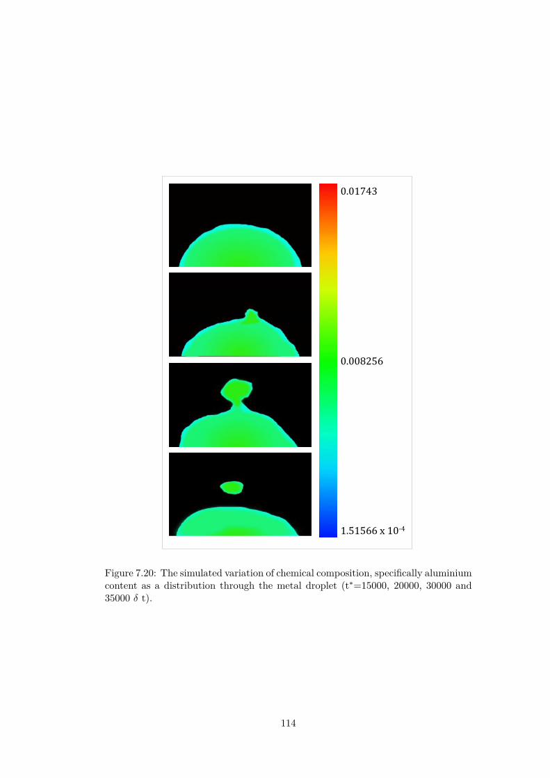
0.01743

0.008256

1.51566 x 10-4

Figure 7.20: The simulated variation of chemical composition, specifically aluminiumcontent as a distribution through the metal droplet (t∗=15000, 20000, 30000 and35000 δ t).

114

1.0

0.6

0.2

Figure 7.21: The gradient of driving force for perturbation growth and breakaway asa combination of chemical free energy and interfacial energy in close time proximitybefore and after material break away (t∗ =20000 and 35000 δ t).

115

7.5 Conclusion

The coupling of experimental techniques and modelling has allowed the in-depth

investigation into the pathway of not only SE in a two-phase system, but also the

life cycle of a perturbation and the limits of size before material breaks away to form

the emulsion. The in-situ observation of emulsification greatly backs the proposal of

hypothesis 5, with spontaneous emulsification being perturbation growth led. The

ability to track these phenomena in ultra-high-temperature systems such as those

presented is of significant importance to directly related fields such as liquid steel

refining of impurity removal such as phosphorus, manganese or silicon. The converse

is also true when considering the ability to predict stable new alloy compositions

with respect to interaction with ladle slags and mould fluxes. In these reactions

knowledge and ability to track the interfacial area between reacting liquid phases

offers the potential for precise control in macroscopic systems where dispersions of

droplets can have significant control over the observed performance. The direct

application of the systems presented here are refining in basic oxygen steelmaking

controlled by emulsion kinetics [37] [53] and the composition control and stability of

lightweight high-aluminium steel grades.

The formation of a physically validated phase-field model to interrogate SE

systems is of great wider value. In addition to the brief summary at the beginning

of this chapter, advanced forms of controllable micro dispersions are under use in

the fields of medicine [116], polymeric nanoparticle production [117] and efficient

recycling of metals [118]. This system is highly dynamic and difficult to capture

reliable first principle data for, due to the extreme temperatures involved. As a

result, reactions and movement can be magnitudes greater than those seen at room

temperature. A greater number of time-step iterations would expectedly be needed

for the model to produce a complete life cycle of an emulsifying system in some of the

slower reacting systems. Although a 3D model of a system is clearer for qualitative

observation and to achieve greater absolute accuracy, the findings in this work show

a 2D phase-field system to have strong experimental agreement, and offer a viable

option when computation time is considered to track the physical phenomena present

in highly dynamic systems over a greater period of time, thus hypothesis 6 is strongly

supported, and the level of accuracy possible to acquire for these systems to date

116

presents a viable data source for the prediction of SE occurrence. It is however

thought the true engineering of geometries through the process would require more

accurate data and development of the model used here.

Despite being able to accurately simulate the interface shape, the phase-field

model is still incapable of reproducing features of the interfacial diffusion. Further

development of the theory is needed to comprehensively understand the interactions

involved in a liquid-liquid interface. An example would be to study whether non-

isothermal effects that may result from latent heat could affect propagation of the

interface. Another direction is to investigate the phenomenological relationships

between diffusion flux and stress tensor. Both expressions were considered to be

isotropic; however, an interface (strong gradients in concentration fields) generates

anisotropy, so the relationships between thermodynamic fluxes and forces should be

reconsidered.

In addition to quantifying the pathway, it is integral to deduce the level of

reaction at the interface required for spontaneous emulsification to occur.

117

Chapter 8

Spontaneous Emulsification as a

Function of Material Exchange


Hypothesis 7: “Within a given system there is a critical point at which spontaneous

emulsification will begin to occur with respect to starting material composition.”

Hypothesis 7 presents the problem of exploring the inflection point of when

emulsification does or does not occur. This will be influenced by the overall flux of

material across the interface and subsequently it is required to quantify the energy

balance between thermodynamic gain against increased interfacial area.

8.2 Introduction

Interfacial tension between molten oxide slurries and liquid steel controls the rate of

reaction where material exchange between the two phases is concerned. The steps

involved in the transfer of material between the two phases are:

1. Mass transfer of a reactive oxide species to the interface in the molten oxide

phase

2. Mass transfer of the reactive element to the interface in the liquid metal phase

3. Interaction of the respective species at the interface

4. Mass transfer of the reaction product away from the interface in the respective

phase

118

The specific system interrogated within the present work is of particular

pertinence in manufacturing due to the social drive of lightweighting in sectors such

as the automobile industry. As a result, the steel industry finds itself in a position

where the development of high aluminium content grades such as TRIP and low

density products is no longer a luxury but a necessity in order to stay competitive

in the market in comparison to materials such as light metals, composites or carbon

fibre.

A high aluminium alloyed steel offers the potential for a stronger lighter ma-

terial in comparison to those currently available. However, such an alloy presents

product issues such as grain refinement due to the lack of phase change, as well as

processing chemical stability with both ladle slurries and mould flux compositions

due to the high SiO2 content favourable for both viscosity and melting point in-

fluences. Processing flow and the addition of material are known to cause droplet

formation of the liquid metal suspended through a protective or partitioning ox-

ide phase, resulting in a large increase in reactive surface area and a potential for

significant material exchange.

In the case of aluminium transfer from liquid steel to a metal oxide phase the

species involved are elemental aluminium and silicon dioxide; the reaction is shown

in equation 8.1

4[Al] + 3(SiO2)→ 3[Si] + 2(Al2O3) (8.1)

where species in [] are in within the liquid metal phase, and those in () are in

the molten oxide phase. In systems such as these, at liquid temperatures it is well

documented that the reactions at the interface are much faster than material mass

transfer within the bulk phases and thus reduction of the diffusion length from bulk

to interfacial reaction site would increase reaction kinetics. This has previously been

reported as a broadening of a metal droplet during sessile drop interrogation [66]

(reduced contact angle) or in the case of an unbound metal droplet mixing of the

two phases into a micro emulsion [62] [86].

With these conditions the reaction rates of a system where a defined first

phase (in this study the metal droplet) is freely suspended in a continuous second

phase (in this study the metal oxide mixture) are limited by the interfacial area/bulk

volume ratio, with the size of the interface (or surface area of a single material) being

a balance between material size, interfacial tension and physical forces.

119

8.2.1 Theoretical Consideration of Interfacial Tension

Interfacial tension (γ) is a balance of the favourable homogeneous phase interactions

as opposed to heterogeneous phase interactions; this is shown through equation 8.2:

γ = (∑

aE1−1i , bE1−1

i+1 , cE1−1i+2 , . . . , xE

1−1i+n )− (

∑dE1−2

i , eE1−2i+1 , fE

1−2i+2 , . . . , yE

1−2i+n )

(8.2)

where E1−1i is the homogeneous phase interaction within the ith solvation

shell; E1−2i is the heterogeneous interaction within the ith solvation shell; and

a, b, c . . . x, y are scaling factors for the number of interactions experienced with each

solvation shell. Within a defined interface a < b and so on for the scale of each

solvation shell. It should be noted from the relationship described in equation 8.2

that interfacial tension can never be zero. Homolytic and heterolytic interaction will

never be equal in energy. If heterolytic interaction is stronger than homolytic then

equation 8.3 would become true:

n∑i

E1−2 >n∑i

E1−1 (8.3)

If this were true there is favourable free mixing of species, there is no defined

interface, only a single phase. From this we see that interfacial tension minimization

is driven by an increase in free energy as atomic interaction energies are fixed for

a given condition. This results in the driving force of surfactant behaviour arising

if possible where heterogeneous interaction between the interfacial location driven

species and a bulk phase is less of an energy cost. For iron and metal oxide two-phase

systems, known atomic interfacial active species of significance are O, S and P in

descending order of influence [119]. The concentration of these species with respect

to interfacial energy reduction has been extensively studied; for example the present

author has shown the driving of this species to an equilibrium state throughout an

industrially relevant system as being a key contributing factor to the spontaneous

emulsification of a metal droplet [62] [86].

As well as the doping of an interface with surfactants, the author will in-

vestigate if material exchange across the interface alone can be enough to reduce

“effective” interfacial tension to a point where physical forces such as Marangoni

120

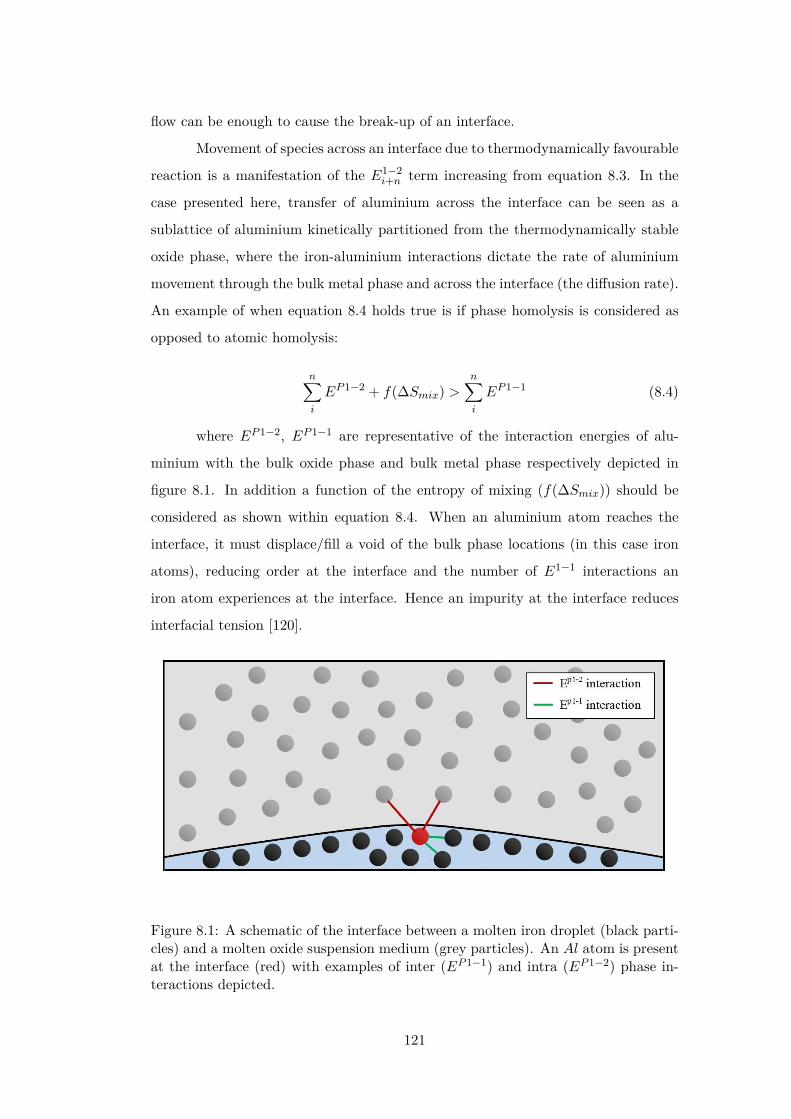
flow can be enough to cause the break-up of an interface.

Movement of species across an interface due to thermodynamically favourable

reaction is a manifestation of the E1−2i+n term increasing from equation 8.3. In the

case presented here, transfer of aluminium across the interface can be seen as a

sublattice of aluminium kinetically partitioned from the thermodynamically stable

oxide phase, where the iron-aluminium interactions dictate the rate of aluminium

movement through the bulk metal phase and across the interface (the diffusion rate).

An example of when equation 8.4 holds true is if phase homolysis is considered as

opposed to atomic homolysis:

n∑i

EP1−2 + f(∆Smix) >n∑i

EP1−1 (8.4)

where EP1−2, EP1−1 are representative of the interaction energies of alu-

minium with the bulk oxide phase and bulk metal phase respectively depicted in

figure 8.1. In addition a function of the entropy of mixing (f(∆Smix)) should be

considered as shown within equation 8.4. When an aluminium atom reaches the

interface, it must displace/fill a void of the bulk phase locations (in this case iron

atoms), reducing order at the interface and the number of E1−1 interactions an

iron atom experiences at the interface. Hence an impurity at the interface reduces

interfacial tension [120].

Figure 8.1: A schematic of the interface between a molten iron droplet (black parti-cles) and a molten oxide suspension medium (grey particles). An Al atom is presentat the interface (red) with examples of inter (EP1−1) and intra (EP1−2) phase in-teractions depicted.

121

In this paper, we will interrogate the starting concentration of aluminium

atoms in the metal drop (which governs the flux of aluminium atoms to the interface)

required to cause sustained perturbation growth on the metal phase surface, as well

as the number required to facilitate spontaneous emulsification of the metal phase

through a molten oxide matrix.

8.3 Experimental

In this investigation seven FeAl alloys were used; their compositions are presented in

table 8.1. The alloys were formed using an open induction furnace with a stock elec-

trically produced “pure” iron chip source and the addition of high-purity aluminium

chips with consecutive addition and sampling of the melt to screen the required com-

positions. All experiments used the same master oxide mixture, the composition of

which is presented in table 8.2. The oxide phase was produced from powder mixing

of the three reagent grade powders followed by pre-melting of the mixture at 1873 K

in a horizontal tube furnace using a gaseous environment of argon (<2 ppm oxygen).

The pre-melting stage was used to ensure full mixing of the oxide compounds, and

was followed by disc milling to form a well-mixed master oxide phase.

Table 8.1: Compositions of FeAl alloys used for the experiments in HT-CSLMpresented in mass %. Compositions were measured by ICP (all alloys contained<0.001 %N).

SampleID

Mn% P% Ni% Cr% Al% C% S% O%

0% Al 0.0003 0.0004 0.0001 0.0003 0.00005 0.004 0.001 0.00341% Al 0.0003 0.0004 0.002 0.0005 0.99 0.0011 0.001 0.00282% Al 0.0004 0.0004 0.001 0.0003 1.92 0.0006 0.001 0.00293% Al 0.0002 0.0004 0.002 0.0005 2.84 0.0011 0.002 0.00354% Al 0.0004 0.0004 0.002 0.0005 3.98 0.0007 0.002 0.00425% Al 0.0003 0.0003 0.002 0.0004 4.92 0.0009 0.002 0.00408% Al 0.0002 0.0004 0.002 0.0005 7.87 0.0007 0.001 0.0038

A high-temperature confocal scanning laser microscope (HT-CSLM) was used

to perform the in-situ observation of the reacting phases. Details on the microscope

can be found in previous reportings [86]. 0.2 g ± 0.02 of the oxide powder was

placed into a sapphire crucible. After placing of the sample inside the HT-CSLM

122

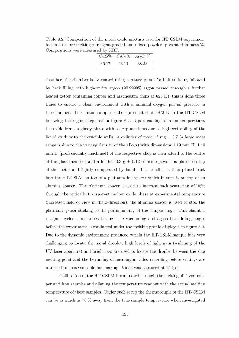
Table 8.2: Composition of the metal oxide mixture used for HT-CSLM experimen-tation after pre-melting of reagent grade hand-mixed powders presented in mass %.Compositions were measured by XRF.

CaO% SiO2% Al2O3%36.17 23.11 38.53

chamber, the chamber is evacuated using a rotary pump for half an hour, followed

by back filling with high-purity argon (99.9999% argon passed through a further

heated getter containing copper and magnesium chips at 623 K); this is done three

times to ensure a clean environment with a minimal oxygen partial pressure in

the chamber. This initial sample is then pre-melted at 1873 K in the HT-CSLM

following the regime depicted in figure 8.2. Upon cooling to room temperature.

the oxide forms a glassy phase with a deep meniscus due to high wettability of the

liquid oxide with the crucible walls. A cylinder of mass 17 mg ± 0.7 (a large mass

range is due to the varying density of the alloys) with dimensions 1.19 mm H, 1.49

mm D (professionally machined) of the respective alloy is then added to the centre

of the glass meniscus and a further 0.3 g ± 0.12 of oxide powder is placed on top

of the metal and lightly compressed by hand. The crucible is then placed back

into the HT-CSLM on top of a platinum foil spacer which in turn is on top of an

alumina spacer. The platinum spacer is used to increase back scattering of light

through the optically transparent molten oxide phase at experimental temperature

(increased field of view in the z-direction); the alumina spacer is used to stop the

platinum spacer sticking to the platinum ring of the sample stage. This chamber

is again cycled three times through the vacuuming and argon back filling stages

before the experiment is conducted under the melting profile displayed in figure 8.2.

Due to the dynamic environment produced within the HT-CSLM sample it is very

challenging to locate the metal droplet; high levels of light gain (widening of the

UV laser aperture) and brightness are used to locate the droplet between the slag

melting point and the beginning of meaningful video recording before settings are

returned to those suitable for imaging. Video was captured at 15 fps.

Calibration of the HT-CSLM is conducted through the melting of silver, cop-

per and iron samples and aligning the temperature readout with the actual melting

temperature of these samples. Under such setup the thermocouple of the HT-CSLM

can be as much as 70 K away from the true sample temperature when investigated

123

0

200

400

600

800

1000

1200

1400

1600

1800

2000

0 100 200 300 400 500 600

Tem

erp

atu

re (

K)

Experimental Time (s)

Experiment Cycle

Pre-melt

Figure 8.2: The nominal heating cycle used for both pre-melting of metal oxides andexperimentation of oxide/metal alloy reaction in the HT-CSLM.

in this manner. Figure 8.2 and reported experimental temperatures are after cali-

bration.

With the use of the semi-transparent sapphire crucibles the physical heating

profile of the HT-CSLM was also investigated. Pieces of thermal paper (similar

to that used in till receipts) cut to size were placed in the base of the crucible on

the stage and spacers. The halogen bulb was then manually turned on for short

periods of time and the resulting heat markings on the paper observed. At low bulb

powers and very short times a 2 mm diameter spot in the centre of the crucible was

observed, this represents the designed focal point of the HT-CSLM chamber. With

incremental increases in time and power exposure, the centre point in the paper

was not seen to grow by an amount observable by eye (due to the poor thermal

conduction of the paper), however a ring around the outside of the crucible was seen

to form and grow inwards. In comparison an opaque crucible such as one of the same

dimensions formed of high-density MgO, did not display the outer heat ring on the

crucible base. It is thought that the transparency of the sapphire crucibles to the

IR wave lengths emitted by the halogen bulb allows for direct heating of a sample

not only from the centre focal point but also from the crucible edges inwards. This

creates a more uniform heat profile through the sample than in previous experiments,

reducing convection and aiding the metal droplet to stay relatively stationary for

viewing during reaction.

124

The videos produced from HT-CSLM experiments have undergone image

processing through grey scale correction to a two-point grey scale, followed by a

segmentation of the image through manual determination of white dictating in-focus

metal phase, and black dictating molten oxide phase. In the case of observation such

as in the first 2% FeAl image for example, the large hollow in the light area of the

droplet image is included in the droplet area segmentation. Data produced from

this method was averaged over 3 frames (the frame each side and the frame of the

time point reported) due to the raster of confocal focus point in the z-plane to give

clearer imaging and greater accuracy in determination of surface area calculation.

Further to this, samples were mounted in resin and sectioned to observe the

quenched material. Figure 8.3 shows the cross sections observed by eye of quenched

samples originally containing the 0%, 3% and 5% FeAl alloys. From these images

we can clearly see that the droplet is suspended in the oxide phase (not on the

surface). In addition, it is qualitatively notable that there is a reduced mass of

material recovered when the initial FeAl content has been increased (a-0%, b-3%

and c-5%). This is expected due to the higher droplet surface area produced during

the experiment allowing for a larger quantity of Fe to be oxidized (causing the metal

phase volume reduction), as well as the additional factor of offspring droplets having

not fully coalesced in the emulsifying systems.

125

Figure 8.3: Images of the sectioned quenched samples showing the droplet suspendedin the oxide phase and the reduction in metal recovery in higher Al content systems.a) 0% FeAl, b) 3% FeAl, c) 5% FeAl.

8.4 Results

Stills of the video output from the HT-CSLM are presented in figures 8.4, 8.5, 8.6,

8.7 and 8.8. These figures correspond to samples 5% FeAl through to 1% FeAl in

respective descending order. Images from 8% FeAl show a very similar behaviour

to that of 5% FeAl, and those of 0% FeAl show a quiescent near-spherical droplet

for the entire period.

Figure 8.4 shows the time-dependent behaviour of the 5% FeAl sample. From

the point at which the droplet is focused upon, perturbation levels are seen to

exponentially increase to a point where the entire field of view is flecked with points

at which perturbations from lower down in the sample have grown into the focal

126

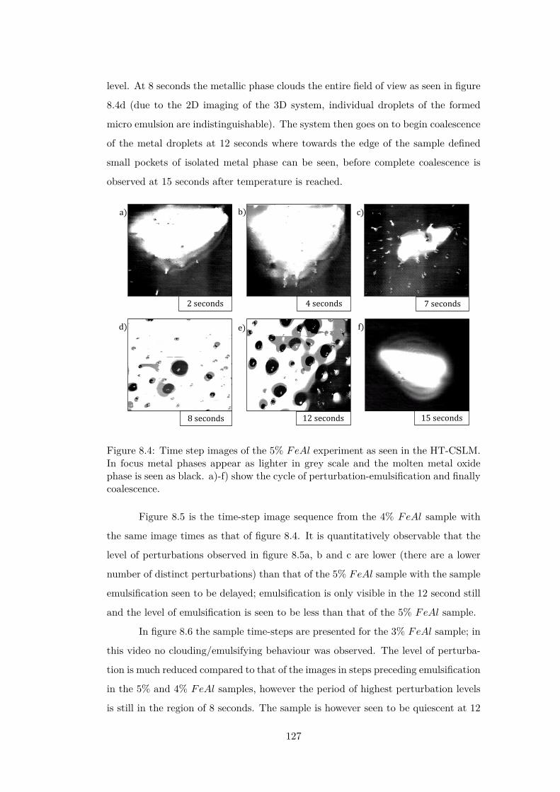
level. At 8 seconds the metallic phase clouds the entire field of view as seen in figure

8.4d (due to the 2D imaging of the 3D system, individual droplets of the formed

micro emulsion are indistinguishable). The system then goes on to begin coalescence

of the metal droplets at 12 seconds where towards the edge of the sample defined

small pockets of isolated metal phase can be seen, before complete coalescence is

observed at 15 seconds after temperature is reached.

a) b) c)

d) e) f)

2 seconds

8 seconds 12 seconds 15 seconds

7 seconds4 seconds

Figure 8.4: Time step images of the 5% FeAl experiment as seen in the HT-CSLM.In focus metal phases appear as lighter in grey scale and the molten metal oxidephase is seen as black. a)-f) show the cycle of perturbation-emulsification and finallycoalescence.

Figure 8.5 is the time-step image sequence from the 4% FeAl sample with

the same image times as that of figure 8.4. It is quantitatively observable that the

level of perturbations observed in figure 8.5a, b and c are lower (there are a lower

number of distinct perturbations) than that of the 5% FeAl sample with the sample

emulsification seen to be delayed; emulsification is only visible in the 12 second still

and the level of emulsification is seen to be less than that of the 5% FeAl sample.

In figure 8.6 the sample time-steps are presented for the 3% FeAl sample; in

this video no clouding/emulsifying behaviour was observed. The level of perturba-

tion is much reduced compared to that of the images in steps preceding emulsification

in the 5% and 4% FeAl samples, however the period of highest perturbation levels

is still in the region of 8 seconds. The sample is however seen to be quiescent at 12

127

2 seconds

a) b) c)

d) e) f)


7 seconds4 seconds

Figure 8.5: Time step images of the 4% FeAl experiment as seen in the HT-CSLM.In focus metal phases appear as lighter in grey scale and the molten metal oxidephase is seen as black. a)-f) show the cycle of perturbation-emulsification and finallycoalescence.

seconds.

a) b) c)

d) e) f)

2 seconds 7 seconds4 seconds


Figure 8.6: Time step images of the 3% FeAl experiment as seen in the HT-CSLM. Infocus metal phases appear as lighter in grey scale and the molten metal oxide phaseis seen as black. a)-f) show the cycle of perturbation growth with no emulsificationseen.

128

The cycle of the 2% FeAl and 1% FeAl samples during reaction can be

seen in figures 8.7 and 8.8 respectively. The images show significantly reduced

levels of perturbation compared to that of the 3% FeAl sample, and a shift of

the highest level of perturbation to earlier in the experimental regime (around 7

seconds). The difference in behaviour is difficult to qualitatively justify from viewing

of the video, however after imaging processing and subsequent measurements being

performed there is a subtle but definite reduction in perturbation level and sustained

perturbation time between the 2% and 1% FeAl samples.

a) b) c)

d) e) f)



Figure 8.7: Time step images of the 2% FeAl experiment as seen in the HT-CSLM.In focus metal phases appear as lighter in grey scale and the molten metal oxidephase is seen as black. a)-f) show the cycle of perturbation growth to quiescentdroplet.

Image processing allows for quantification of the liquid metal surface area

as seen in the 2D images of the HT-CSLM. Figure 8.9 displays the relative metal

surface area change as a function of time for all seven experiments (extrapolated

back to zero time assuming a quiescent sphere is formed on first melting). The

measurements of the images displayed in figures 8.4-8.8 are highlighted.

From figure 8.9 we can see the 2D image analysis has led to distinct profiles

for different levels of Al in the metal droplets. Both 8% and 5% FeAl samples show

an emulsification profile near 10 times the original surface area of an ideal droplet

(spherical shape) at its highest point; they both peak at 8 seconds. The 4% FeAl

129

a) b) c)

d) e) f)



Figure 8.8: Time step images of the 1% FeAl experiment as seen in the HT-CSLM.In focus metal phases appear as lighter in grey scale and the molten metal oxidephase is seen as black. a)-f) show the cycle of perturbation growth to quiescentdroplet.

0

2

4

6

8

10

12

0 5 10 15 20

Rel

ativ

e su

rfac

e ar

ea (

A1

/A0

)

Experimental time at 1873 K (s)

8% FeAl

5% FeAl

4% FeAl

3% FeAl

2% FeAl

1% FeAl

0% FeAl

Figure 8.9: The surface area ratio profiles as deduced from image analysis of theHT-CSLM video (to the nearest 0.05). 1 in 15 frames have been analysed but onlythe points corresponding to those in figures 8.4-8.8 are highlighted.

sample still shows emulsification behaviour to a lesser extent, with a maximum of

near 7 times an ideal droplet; this maximum does however come significantly later

in the reaction process. Samples of 3%, 2% and 1% FeAl show much lower levels

of surface area increase, with less perturbation than the higher aluminium content

130

alloys and no emulsification behaviour. Although not visible due to scale on the

graph here, there is a trend of end-point surface area ratio being below 1, with

samples that emulsified having a lower ratio than those that didn’t. This reduction

in size is due to the oxidation of the sample/dissolution into the slag phase. Samples

which emulsified have much larger surface area not only for aluminium refinement

but also for oxidation of the bulk iron phase, meaning greater loss of material (as

previously depicted in figure 8.3).

8.5 Discussion

Figures 8.4-8.8 clearly depict the change in droplet morphology lifecycle when alu-

minium content is reduced in the metal droplet. The quantification of surface area

change shown in figure 8.9 offers clarification of four behaviours. The 8% and 5%

FeAl samples show exponential increase in surface area between 7 and 8 seconds.

This large increase in area over such a short period shows true spontaneous emul-

sification behaviour; the droplets effectively tear themselves apart into the micro-

emulsion of smaller droplets. This may be indicative of breakaway droplets further

breaking down due to the large chemical potential in place across the interface. The

4% FeAl sample shows a similar level of emulsification to the higher aluminium

content samples, however the peak in surface area is later into the reaction cycle

and the increase is more gradual. A method by which this would happen is if the

budding of perturbations on the droplet surface continued to occur at a faster rate

than any coalescence; rather than a sudden break down of the droplet there is a

gradual release of offspring droplets through the reaction period.

Although the 8%, 5% and 4% FeAl samples show differing emulsification

profiles, the coalescence behaviour is very similar. Due to the differing time scales

for emulsification to occur, the severity of emulsification and the sustained chemical

potential across the interface in the offspring droplets aluminium content is reduced

at a faster rate in the metal droplet at higher original aluminium content. So much

so that we see all emulsifying systems coming to a quiescent droplet within a very

close time proximity.

Riboud and Lucas [99] conducted similar experiments where a larger iron-

aluminium alloy droplet was observed via X-ray radiography. Their results were

131

recorded over a much longer time period (around 50 minutes), and their interpreted

interfacial tension between metal and oxide phase during the observation is reported.

They follow the workings of Defay, Sanfeld, Steinchen and Friedel [121] [122] [123],

where a model of equidistant planes parallel to the interface containing the molecules

is considered against a perpendicular z diffusion axis. In this model they discuss a

mechanical equilibrium expression for interfacial tension such that:

γ = e3∫ b

a

∑x

∑x′

kxx′c′xc′x′dz (8.5)

where kxx′ is the attraction between molecules x and x′ situated in a layer

thickness e; c′x = dcy/dz and c′x′ = dcy′/dz are the concentration gradients along

the z-axis; a and b are positions on the z-axis in two phases A and B far enough

from the interface that c′y and c′y′ are negligible. This results in a discussion of

interfacial tension being zero when there exists a pair of concentration gradients

with opposite signs and heterogeneous interactions are greater in strength than

homogeneous interactions. Although this is similar to the treatment of interfacial

tension discussed in the opening arguments, there is a fundamental difference where

the current work considers this movement of favourable exchange between phases to

be a sublattice exchange; this is not the mixing of the two bulk phases. If two bulk

phases still exist, there must be a net positive interfacial tension.

This being said the trend of interfacial tension change does not change, only

the absolute values. These values are incomputable from the data collected in this

study, however if the trend reported by Riboud and Lucas [99] is corrected for time

scale due to the miniaturization of the present study the interfacial tension coincides

well with the interfacial area changes in current systems, with the spontaneity of

emulsification and coalescence captured. There is a delay of surface tension increase

in comparison to that of interfacial tension in the earlier study which is thought to

be caused by the heating performance of the HT-CSLM. During these early stages

the sample in the HT-CSLM may be below the programmed temperature of 1873

K and spatially heterogeneous with regards to temperature, this would cause the

reaction between aluminium and SiO2 to be hindered.

Both Riboud et al [99] and Rhamdhani et al [63] [64] [65], present the most

directly relevant system reports in the literature previously. The major experimental

132

differences between the three studies are: Riboud [99] uses a larger droplet dimen-

sion (0.5-2 g) and the experiment is akin to in-situ x-ray observation of a sessile

experiment, the droplet is in contact with a substrate at all times; Rhamdhani [63]

uses a larger droplet dimension (1.7-3.25 g), with the droplet suspended in the oxide

medium and samples were quenched and crushed for evaluation; the present study

uses smaller droplets (17 mg ± 0.7), suspended in the oxide medium observed in-situ

via a scanning UV laser.

The first consideration for analysing the effects of experimental differences is

the pathway of perturbation growth and budding of the system. Perturbations ini-

tially grow due to the shortening of diffusion distance to reactive species in the bulk

oxide phase. Figure 8.10 offers a schematic tool to explain this, where: a) depicts

the diffusion distance for SiO2 to reach the perturbation head from the bulk oxide

phase; b) depicts the diffusion distance for SiO2 to reach the perturbation length

centre (and at a later stage the neck of a perturbation); c) depicts diffusion distance

for SiO2 to reach the main droplet body. As material is reacted the perturbation

growth is sustained through entering areas of the bulk oxide phase where SiO2 is still

enriched; this microscopic growth phenomena reduces the diffusion length required

for new SiO2 molecules to reach the interface. The sustained growth/increase in

surface area is energetically rationalised by the increase in material exchange be-

tween the two phases; the Gibbs free energy is still reducing in the overall system.

As the perturbation grows distance a) is maintained, and distance c) is maintained,

but the effective distance b) (distance from the perturbation centre to the bulk oxide

phase) is increased due to depressed levels of SiO2 in the oxide bulk phase through

which the perturbation front has previously grown. This creates a profile of reaction

potential down the perturbation, with higher chemical potential in the perturbation

head and lower chemical potential further down the direction of growth. This re-

sults locally in a necking phenomenon as the advancing perturbation head growth is

sustained while there is much less drive for increased width close to the main droplet

body. This results in the development and gradually increasing severity of the angle

labelled θ on figure 8.10. We can add this geometric constraint to the expression for

interfacial tension presented earlier in this work, together with mixing drive in the

system, to give an expression for inter-phase tension γp:

133

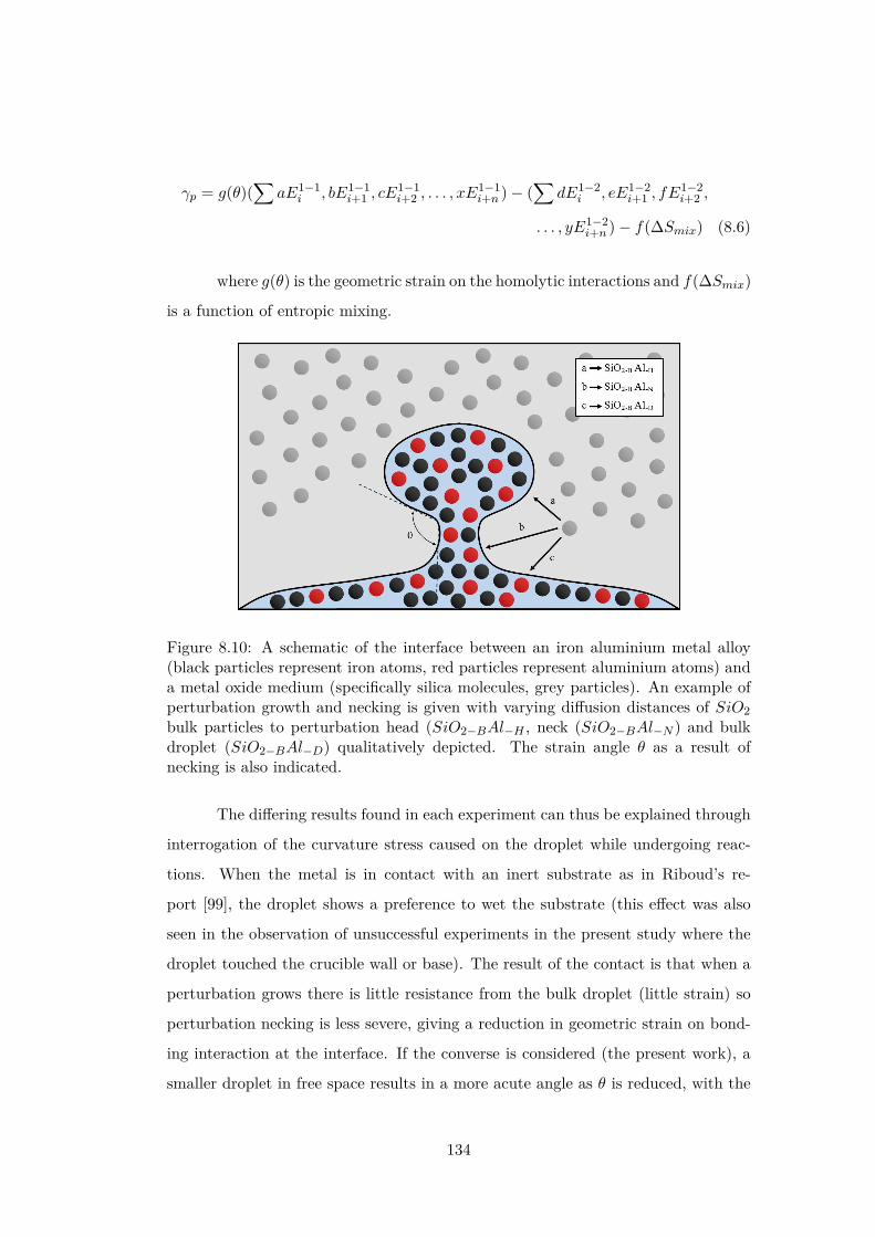
γp = g(θ)(∑

aE1−1i , bE1−1

i+1 , cE1−1i+2 , . . . , xE

1−1i+n )− (

∑dE1−2

i , eE1−2i+1 , fE

1−2i+2 ,

. . . , yE1−2i+n )− f(∆Smix) (8.6)

where g(θ) is the geometric strain on the homolytic interactions and f(∆Smix)

is a function of entropic mixing.

Figure 8.10: A schematic of the interface between an iron aluminium metal alloy(black particles represent iron atoms, red particles represent aluminium atoms) anda metal oxide medium (specifically silica molecules, grey particles). An example ofperturbation growth and necking is given with varying diffusion distances of SiO2bulk particles to perturbation head (SiO2−BAl−H , neck (SiO2−BAl−N ) and bulkdroplet (SiO2−BAl−D) qualitatively depicted. The strain angle θ as a result ofnecking is also indicated.

The differing results found in each experiment can thus be explained through

interrogation of the curvature stress caused on the droplet while undergoing reac-

tions. When the metal is in contact with an inert substrate as in Riboud’s re-

port [99], the droplet shows a preference to wet the substrate (this effect was also

seen in the observation of unsuccessful experiments in the present study where the

droplet touched the crucible wall or base). The result of the contact is that when a

perturbation grows there is little resistance from the bulk droplet (little strain) so

perturbation necking is less severe, giving a reduction in geometric strain on bond-

ing interaction at the interface. If the converse is considered (the present work), a

smaller droplet in free space results in a more acute angle as θ is reduced, with the

134

perturbation neck merging with the main droplet curvature. This creates high levels

of strain at the perturbation neck. This strain along with the system free energy can

be stabilized by the physical detachment of the perturbation head from the main

droplet body. This is the phenomenon we refer to as budding.

The levels of perturbation/emulsification follow this trend through Riboud

and Lucas [99] who report a wavy quenched interface geometry for a sample in

the middle of the reaction; Rhamdhani et al [64] reported some material break up

through the discovery of several metal droplets of varying sizes in the quench sample;

the present work shows full emulsification of the higher aluminium content samples,

but also behaviour similar to those of larger droplets when lower aluminium contents

are investigated (this is due to the reduction in perturbation growth speed, giving

greater time for diffusion of SiO2 towards the perturbation length centre, reducing

the impact on necking severity).

As stated earlier, the time taken to reach a quiescent droplet interface at/near

equilibrium is greatly reduced in the current work in comparison to that of Riboud

and Lucas [99]. This is expected to be due to three reasons: 1) the droplet being

much smaller, 2) spontaneous emulsification occurring, greatly increasing the surface

area/volume ratio, and 3) an unbound droplet being able to grow perturbations into

new bulk composition areas of oxide phase in all directions. These factors change

the probable rate controlling step from SiO2 mass transport in the earlier reported

work to Al mass transport in the current findings.

The effect of oxygen concentration in the metal droplet of similar two-phase

systems is well documented by several authors [92] [119] [124] [125] [126]. Reports

range from a surface tension of close to 1500 mN m−1 at near zero oxygen content

and follow an exponential decay in interfacial tension to values of near 400 mN m−1.

From previous discussion we know barriers close to the lower end of this spectrum

are possible to overcome and emulsification occurs to a high degree [62] [86].

This allows us to confirm that interfacial tension of the 3%, 2% and 1%

FeAl samples did not reach levels as low as 400 mN m−1 as emulsification did not

occur. Further to this, the current study contains no FeO in the oxide phase, a key

agent in the provision of oxygen content for low interfacial tension. Although we

cannot bound the interfacial tension for higher levels of aluminium, it is improbable

when considering the behaviour shown with oxygen content that a 1% increase in

135

aluminium content would drastically reduce the interfacial tension to a near zero or

negative value.

In an effort to quantify the interfacial tension through visualization of spon-

taneous emulsification performance, it is thought a future investigation where iron

(II) oxide content is varied in the oxide phase of experiments in the HT-CSLM could

be used to validate interfacial tension in systems undergoing transport of material

across the interface.

To quantify the reasoning behind the inflection point in emulsification be-

haviour of the varying FeAl content alloys, an investigation into the energy balance

of free energy dissipation competing with the increased global interfacial tension due

to increasing surface area is performed (values for calculations given in table 8.3).

Using the interfacial areas measured for 8% FeAl, (deemed the standard emulsifica-

tion behaviour) and an interfacial tension of 1500 mN m−1 as a realistic maximum

from the literature [91], the energetic cost of interfacial area change with time can

be calculated with use of equation 8.7 as shown in figure 8.11:

SIT = IAxIT (8.7)

where SIT is the energy cost of sustaining the interface between metal and

oxide in the system, IA is the interfacial area between metal and oxide phases and

IT is the interfacial tension.

Table 8.3: Literature values used for calculation of global interfacial tension anddissipation of free energy as displayed in figure 8.11.

Interfacial Tension 1500 mN m−1

∆HFormationAl2O3 -1669.8 kJ mol−1

∆HFormationSiO2 -859.4 kJ mol−1

SAl2O3 50.92 J mol−1 K−1

SSiO2 42.0 J mol−1 K−1

CpAl2O3 880 J Kg−1 K−1

CpSiO2 680 J Kg−1 K−1

Temperature 1873 K

The total dissipation of free energy due to reaction for each level of aluminium

content is then also calculated with use of equation 8 and displayed in figure 8.11:

136

0

5E-11

1E-10

1.5E-10

2E-10

2.5E-10

3E-10

3.5E-10

4E-10

4.5E-10

0 2 4 6 8 10 12 14 16 18

En

ergy

(J)

Experimnental Time at 1873 K (s)

InterfacielTension

8%

5%

4%

3%

2%

1%

AB

C

D

E

Global It

Figure 8.11: Global interfacial tension during the increase and reduction of inter-facial area as measured for the 8% FeAl sample coupled with the free energy gainof reaction to equilibrium for the 8, 5, 4, 3, 2, and 1% FeAl systems. Period A isduring initial light perturbation, B during heavy perturbation, C fully emulsified, Dongoing coalescence and E a fully coalesced droplet.

∆G = ∆H∗ − TδS (8.8)

where G is the Gibbs free energy, H∗ the reaction enthalpy calculated using

Kirchhoff’s Law, T is the temperature and S is the reaction entropy.

Input values for these calculations are also presented in table 3. At 8 seconds,

the point of highest emulsification level observed in the higher aluminium content

samples is pin pointed in the centre of the global It curve (zone C), with the free

energy gain of the 4% FeAl sample just slightly higher. This agrees well with the

experimental observations as up to zone C the surface area is growing (through

regions A and B where perturbation begins, and grows), and thus a driving force

for the spontaneous emulsification cycle is required. After point C we have gradual

coalescence of the metal phase defined by D, restricted through statistical colocation

of material and restraints such as film drain barriers (previously discussed to be

dictated in a pathway well described by DVLO theory [62]). Thus after 8 seconds

the surface area is unstable. There is no longer a driving force for a sustained

interfacial area. Finally, the reaction reaches point E where the droplet has fully

coalesced. Although 4% FeAl is above the energy required to develop the fully

137

emulsified state, it is extremely close in energy levels required. This may explain

the prolonged time, and reduced level of emulsification seen compared to the higher

levels of FeAl which exhibit more similar behaviour to each other.

8.6 Conclusions

The effect of aluminium content on the transient interface morphology between iron

aluminium alloy droplets and an enriched silicon oxide phase has been studied in-

situ with use of a HT-CSLM. The behaviour shows an inflection between 4% and

3% FeAl content samples evaluated through the surface area determination of the

metal phase as analysed via automated post-experiment image analysis.

A discussion is given into the nature of interfacial tension where previously

reported near-zero and negative interfacial tension energies are deemed unrealistic,

with an alternative interpretation of the system treatment given to account for the

phenomena observed.

The physical manifestation of interfacial energy change is discussed with

regards to the severity of necking behaviour. This is used to evaluate the differences

seen in metal morphologies between the current findings reported here and those

previously reported in the literature of the most relevant systems.

Finally, an interrogation of the energy balance between free energy dissipation

of reaction and interfacial tension cost is given. The inflection point in behaviour

relative to the aluminium content can be seen to straddle the energy cost of inter-

facial area increase between the 3% and 4% FeAl samples. Presenting an energetic

reasoning to the observations given.

The nature of the results show hypothesis 7 to be true, and the exploration

of energetic gain through reaction is seen to be a reasonable explanation for the

change in behaviour. In addition, below the critical point of emulsification, there is

still variation in behaviour, manifesting in these findings as the level to which the

metal droplet surface perturbs; to a large extent at 3% aluminium, with reducing

levels through 2%, 1% and 0% aluminium.

138

Chapter 9

Conclusions and Suggested

Further Work

9.1 Conclusions

9.1.1 Macroscopic Dynamics

With the use of pilot plant data in chapter 5 a model for the calculation of residence

time, metal circulation rate and % tap weight in the emulsion phase has been created

for a BOF. The assumptions have been interrogated through critical assessment in

comparison to previous literature, as well as new analytical XCT data with regard

to the potential for decarburization in the emulsion phase through metal droplets.

Points of high residence time draw correlation with high bulk dephosphoriza-

tion, whereby it is reasonable to state that dephosphorization is driven through the

emulsion droplet interaction with slag. However, even though there is a reasonable

trend in decarburization, the calculation of possible decarburization in the emulsion

fell short (∼ 60%) of the overall decarburization rate seen at times.

Metal circulation rate is seen to gradually increase with time, until end-blow

periods where the level of decarburization is reduced, slag foaming collapses and

droplets are likely to take on a more direct flight trajectory through the gas phase

above the collapsed slag layer rather than through the previously stabilized emulsion.

These factors couple to cause droplets to move faster/experience less hindrance to

their movement in the late blow.

% Tap weight in the emulsion is seen to be considerably higher than is re-

139

ported in most previous literature, giving further credence to the process being

driven by material in the emulsion phase. There is however little to comment on

trends within these findings: some heats appear to gradually increase; some stay

relatively stable; and others show erratic behaviour throughout the blow. The main

point to take however, is that there does not seem to be an overall reduction in

metal within the emulsion for any heat between start and end values.

Overall the formulation of this macroscopic model gives a successful output

and builds upon previous knowledge both direct from IMPHOS findings and the

wider literature. It should however be noted that this study was on a 6 ton pilot

scale, where all factors are scaled down apart from the velocity of the oxygen jet,

which was still supplied at Mach 2 in resemblance to industrial practice. Factors

such as a reduced vessel cross section, reduced material masses and reduced potential

flight path (both horizontally and vertically) must be taken into serious consideration

when these findings are considered at an industrial scale.

9.1.2 Driving Force of Spontaneous Emulsification

The chemical analysis of samples from FeP − FeO reactive droplet systems has

been conducted. The results show clearly that the phosphorus reaction was likely

uninvolved in the emulsification process. In addition, SEM-SIMS was conducted to

quantify oxygen levels in the droplet during the emulsification profile. It was found

that the oversaturation of oxygen in the droplet and the re-equilibration of this

transferring back to the slag phase was the likely cause of the phenomenon. This was

backed up through the investigation of a zero P system, where again emulsification

was witnessed. However, the emulsification profile was seen to be displaced from the

original FeP − FeO findings, which could well have been due to the additional P

removal driving force in the initial phases of the experiment. Though, it would be

crude to draw definition on this statement as HT-CSLM experiments are sensitive

to usage variation through packing of slag, and maintenance of the chamber.

Further to this, the in-situ observation of the spontaneous emulsification

phenomena through the use of FeAl−SiO2 systems show initial aluminium content

to cause the development of differing behaviour. The spontaneity and severity of

emulsification showed reduction at 4% aluminium content and was further reduced

to a non-emulsifying system at 3% aluminium.

140

The energy balance of increased interfacial area cost with the free energy

dissipation of reaction is then considered. A clear relationship between the two

can be seen to account for the occurrence of emulsification or lack thereof. In

addition the level of free energy dissipation can be seen to be relative to the severity

of perturbation growth in the non-emulsifying systems. This is a key finding in

understanding the possibility for a system to emulsify or not.

9.1.3 Physical Pathway of Spontaneous Emulsification

Observations of emulsifying systems in low and high magnification show clearly a

perturbation growth-driven pathway for emulsification. Theory is developed as to

why perturbations grow, neck and bud, through a diffusion length lead argument.

In addition, with the use of XCT and HT-CSLM image analysis the interfacial area

increase during perturbation and emulsification is given; this is a key variable in the

interfacial transfer pathway many elements are refined through during steelmaking.

High-resolution XCT of quenched perturbed samples allowed for the quan-

tification of average perturbation growth size with respect to reaction time and a

clear change in perturbation lifecycle profile is reported. The findings show that

perturbations will grow in a 1:1 ratio untill 200 µm when necking occurs and a fi-

nal maximum perturbation length of 470 µm before material breaks away from the

parent droplet. The knowledge of how emulsification manifests gives insight into

the parameters requiring control to predict and engineer the formation of a desired

micro-emulsion.

Further to this, phase-field modelling techniques have been developed to in-

corporate the correct driving force and fluid mechanics to be able to map emulsifica-

tion in two and three dimensions with respect to time. The linking of experimental

techniques with modelling allows for the rationalization of a Fourier based modelling

approach.

9.2 Potential Industrial Impact

The cumulative findings from this work have direct implication when considering

the transient interfacial area during BOS processing. The macroscopic dynamics

deduced through novel treatment of an extensive data set presents findings in a

141

format allowing industry to fully appreciate the conditions and assumptions the

results apply to. Specifically the residence times reported show strong consistency

with those of model output in the literature, giving credence to the finding as well

as information on how this parameter changed throughout the blow.

Results from the metal/slag HT-CSLM experiments show an individual droplet’s

surface area may increase by 10 times during a reactive process. When you consider

at the time over half the total metal was found to be in droplet form within the

emulsion phase of the BOF, this has the potential to greatly affect refining perfor-

mances in the BOF, as well as the rate of reactions in ladles, the tundish, or even

during casting.

Specifically these experiments do not include carbon as a reacting species,

which is known to cause bloating and gas halos from the produced gases [35]. When

we consider this, the low levels of carbon in the BOF towards end blow, and the po-

tential for high levels of metal suspended in the slag phase with rising temperatures;

potentially there is evidence as to why phosphorus reversion may occur.

9.3 Suggested Further Work

The following points give suggestions for future work to build on the current findings

within this project:

1. Introduction of carbon to the spontaneous emulsification experiments. This

would give a system with direct comparison to a significant profile of work in

the literature as a technique validation.

2. Introduction of tertiary alloys to the emulsification experiments. This would

allow for the observation of effects such as either interfacial site blocking or

gas evolution to see which reactions are dominant in the cause of the observed

phenomena. A prime example would be an Fe − C − P droplet, where the

evolution of a gas halo may inhibit dephosphorization/the flux of oxygen into

the droplet and an inflection in behaviour from decarburization to dephospho-

rization led behaviour may be witnessed.

3. Continued development of the phase-field model presented, where the level

of material movement can be interrogated to test the drive and extent of

142

emulsification similar to the results seen in the variable FeAl profile of work.

Once validated in this fashion the phase-field model should offer a robust

prediction method for binary alloys. A key variable to explore would be the

effect of changing FeO content in the slag phase.

4. The use and incorporation of data from more experimentally complex alloy

systems to see how competing reactions affect each other (as discussed in

point 2) would offer information required for the phase-field model to make

the final step into an invaluable tool for informing slag/metal reactions.

5. Further use of XCT to interrogate quenched emulsion samples from the IM-

PHOS converter would allow for a robust droplet size distribution measure-

ment in both a converter height profile and blow time profile. This has timely

pertinence to many BOF modelling approaches being undertaken globally to-

day (droplet size distribution is key to defining both the interfacial area and

the governing behaviour of metal size fractions in the BOF emulsion).

6. Further additions of information to the macroscopic dynamic model are re-

quired to improve its accuracy. Addition of decarburization potential assigned

to both the bulk bath and hot zone would improve calculation accuracy.

7. Finally, if the above scheme of work were to be conducted, it’s combination

along with processing parameter effects from the literature would offer the po-

tential to truly understand and predict refining performance within the BOF.

143

Bibliography

[1] World Steel Association. World Steel Association Yearbook. Technical report,

2016.

[2] H. Tanabe and M. Nakada. Steelmaking technologies contributing to steel

industries. NKK Technical Review(Japan), 88(88), 2003.

[3] M. De Graef and M.E. McHenry. Structure of Materials: An Introduction to

Crystallography, Diffraction and Symmetry. 2012.

[4] M.S. Millman, A. Kapilashrami, M. Bramming, and D. Malmberg. Imphos:

improving phosphorus refining. Technical report, European Commision: Re-

search Fund for Coal and Steel (RFCS), Brussels, 2011.

[5] D.C. Copley, J.W. Eberhard, and G.A. Mohr. Computed tomography part I:

introduction and industrial applications. JOM, (January), 1994.

[6] T. Matsumiya. Steelmaking technology for a sustainable society. Calphad,

35(4):627–635, Dec 2011.

[7] U. Martin. Integrated Mill. Technical report, viewed 2017.

[8] E.T. Turkdogan. Physiochemical Aspects of Reactions in Ironmaking and

Steelmaking Processes. ISIJ, 24, 1983.

[9] L.J. Westholm. The Use of Blast Furnace Slag for Removal of Phosphorus

from Wastewater in Sweden - A Review. Water, 2(4):826–837, Oct 2010.

[10] W.J.B. Chater. Oxygen processes in the steel industry. Chemical Engineering

Science, 3:105–IN5, Jan 1954.

144

[11] H. Yi, G. Xu, H. Cheng, J. Wang, Y. Wan, and H. Chen. An Overview of

Utilization of Steel Slag. Procedia Environmental Sciences, 16:791–801, Jan

2012.

[12] M. Han and Y. Zhao. Dynamic control model of BOF steelmaking process

based on ANFIS and robust relevance vector machine. Expert Systems with

Applications, 38(12):14786–14798, Nov 2011.

[13] United States Environmental Protection Agency. Available and Emerging

Technologies for Reducing Greenhouse Gas Emissions from the Iron and Steel

Industry. Technical Report September, United States Environmental Protec-

tion Agency, 2012.

[14] M. Wang, Y. Lu, W. Yang, S. Li, and X. Xu. Selection of Oxygen Pres-

sure in BOF Steelmaking. Journal of Iron and Steel Research, International,

18(11):12–16, Nov 2011.

[15] Z. Tian, B. Li, X. Zhang, and Z. Jiang. Double Slag Operation Dephospho-

rization in BOF for Producing Low Phosphorus Steel. Journal of Iron and

Steel Research, International, 16(3):6–14, May 2009.

[16] M. Swinnerton. The influence of slag evolution on BOF dephosphorisation.

PhD thesis, University of Wollongong, 2005.

[17] S. Kitamura, K. Miyamoto, H. Shibata, N. Maruoka, and M. Matsuo. Anal-

ysis of Dephosphorization Reaction Using a Simulation Model of Hot Metal

Dephosphorization by Multiphase Slag. 95:313–320, 2009.

[18] M. Muhammed and Y. Zhang. A hydrometallurgical process for the dephos-

phorization of iron ore. Hydrometallurgy, 21:277–292, 1989.

[19] B.J. Monaghan, R.J. Pomfret, and K.S. Coley. The kinetics of dephospho-

rization of carbon-saturated iron using an oxidizing slag. Metallurgical and

Materials Transactions B, 29(February):29–32, 1998.

[20] G. Hayman and D.A. Denton. Process heating, power and incineration.

(July):1997, 1997.

145

[21] S. Emea. Some Observations on BOS Refining. Ironmaking & Steelmaking,

pages 1–17, 2009.

[22] C.P. Manning and R.J. Fruehan. The rate of the phosphorous reaction between

liquid iron and slag. Metallurgical and Materials Transactions B: Process

Metallurgy and Materials Processing Science, 44(1):37–44, 2013.

[23] C. Cicutti, M. Valdez, T. Perez, J. Petroni, A. Gomez, R. Donayo, and

L. Ferro. Study of Slag-Metal Reactions in an LD-LBE Converter. In 12

IAS Steelmaking Seminar, volume 250, 1999.

[24] American Iron and Steel Institute. The Basic Oxygen Steelmaking (BOS)

Process. Technical report, viewed 2017.

[25] R.M. Smailer. Phosphorus Control in DRI. In ILFA Congress, Mexico City,

1983.

[26] M.Y. Mohassab-Ahmed, H.Y. Sohn, and H.G. Kim. Phosphorus Distribution

between Liquid Iron and Magnesia-Saturated Slag in H2/H2O Atmosphere

Relevant to a Novel Ironmaking Technology. Industrial & Engineering Chem-

istry Research, 51(20):7028–7034, May 2012.

[27] C. Solans, D. Morales, and M. Homs. Spontaneous emulsification. Current

Opinion in Colloid and Interface Science, 22:88–93, 2016.

[28] N. Sano and P.V. Riboud. Advanced physical chemistry for process metallurgy.

Academic Press, 1997.

[29] M.A. Tayeb, R. Fruehan, and S. Sridhar. De-phosphorization in the DRI-EAF

steelmaking and the effect of alumina. In AISTech, page 1, 2014.

[30] M.A. Tayeb, R. Fruehan, and S. Sridhar. Phosphorus partitioning during

EAF refining of DRI based steel. In International Symposium on Liquid Metal

Processing & Casting, pages 353–358, 2013.

[31] D. Wang. A novel method for controlling the surface morphology of polymeric

membranes. Journal of Membrane Science, 169(1):39–51, 2000.

146

[32] M.S. Millman, A. Overbosch, A. Kapilashrami, D. Malmberg, and

M. Bramming. Some observations and insights on BOS refining. Ironmak-

ing & Steelmaking, 40(6):460–469, Aug 2013.

[33] B.J. Monaghan. Kinetics of Liquid Iron Dephosphorization Using Lime Based

Slags. PhD thesis, University of Stathclyde, 1996.

[34] H.P. Mattila, I. Grigaliunaite, and R. Zevenhoven. Chemical kinetics modeling

and process parameter sensitivity for precipitated calcium carbonate produc-

tion from steelmaking slags. Chemical Engineering Journal, 192:77–89, Jun

2012.

[35] K.S. Coley and G. Brown. Kinetics of BOF Steelmaking. In International

Conference on the Technology of Ironmaking and Steelmaking, Jamshedphur,

India, 2014.

[36] E. Chen. Kinetic Study of Droplet. PhD thesis, McMaster University, 2012.

[37] H.W. Meyer, W.F. Porter, G.C. Smith, and J. Szekely. Slag-Metal Emulsions

and their Importance in BOF Steelmaking, 1968.

[38] D.J. Price. L.D. Steelmaking: Significance of the emulsion in carbon removal.

In Process Engineering of Pyrometallurgy, pages 8–15. 1974.

[39] R.F. Block, A. Masui, and G. Stolzenberg. Physical Processes in the Top

Blown Oxygen Converter. Arch Eisenhuttenwes, 44:p357–361, 1973.

[40] R.C. Urquhart and W.G. Davenport. Foams and emulsions in oxygen steel-

making. Canadian Metallurgical Quarterly, 12(4):507–516, 1973.

[41] O.K. Tokovoi, A.I. Stroganov, and D.Y. Povolotskii. Tokovoi. Steel USSR,

pages 116–117, 1972.

[42] W. Resch. Kinetics of P Removal During O Top-Blowing Processes for P-Rich

Fe. Ph.d thesis, Technical University, Clausthal, 1976.

[43] V.I. Baptizmanskii, V.B. Okhoskii, K.S. Provirin, G.A. Shcherdrin, Y.A.

Ardelyan, and A.G. Velichko. Investigation of the Physico-chemical Processes

in the Reaction Zone with Oxygen Injection of the Metal. Steel USSR, 7:p329–

331, 1977.

147

[44] S.C. Koria and K.W. Lange. A new approach to investigate the drop

size distribution in basic oxygen steelmaking. Metallurgical Transactions B,

15(March):109–116, 1984.

[45] S.C. Koria and K.W. Lange. Breakup of Iron-Carbon Drops by a High Velocity

Oxygen Gas Jet. Canadian Metallurgical Quarterly, 18(2):131–143, 1979.

[46] S.C Koria and K.W. Lange. Estimation of drop sizes in impinging jet steel-

making processes. Ironmaking and Steelmaking, 13(5):236–240, 1986.

[47] J. Gustavsson. Reactions in the Lower Part of the Blast Furnace with Focus

on Silicon. PhD thesis, Royal Institute of Technology, 2004.

[48] Q. He. Fluid Dynamics and Droplet Generation in the BOF Steelmaking Pro-

cess. PhD thesis, University of Wollongong, 1991.

[49] K.C. Mills, E.D. Hondros, and Z. Li. Interfacial phenomena in high tempera-

ture processes. Journal of Materials Science, 40(9-10):2403–2409, 2005.

[50] Subagyo, G.A. Brooks, and K.S. Coley. Residence time of metal droplets in

slag-metal-gas emulsions through top gas blowing. Canadian Metallurgical

Quarterly, 44:119–130, 2005.

[51] P. Kozakevitch. Foams and Emulsions in Steelmaking. Journal of Minerals,

Metals and Materials Society, 22(7):57–58, 1969.

[52] G. Brooks, Y. Pan, and K. Coley. Modeling of trajectory and residence time

of metal droplets in slag-metal-gas emulsions in oxygen steelmaking. Metal-

lurgical and Materials Transactions B, 36(August), 2005.

[53] Q.L. He and N. Standish. A model study of residence time of metal droplets

in the slag in BOF steelmaking. ISIJ International, 30(5):356–361, 1990.

[54] N. Dogan and G.A. Brooks. Comprehensive Model of Oxygen Steelmaking

Part 2 : Application of Bloated Droplet Theory for Decarburization in Emul-

sion Zone. ISIJ International, 51:1093–1101, 2011.

[55] M. Pomeroy. Droplet decarburization kinetics in steelmaking slags. PhD thesis,

McMaster University, 2011.

148

[56] K. Coley, F. Ji, G. Brooks, M. Rhamdhani, and Y. Pan. The Interface in Slag

Reactions; a Moving Target. Researchbank.Swinburne.Edu.Au, 2009.

[57] B. Deo, A. Karamcheti, and A. Paul. Characterization of slag-metal droplet-

gas emulsion in oxygen steel making converters. ISIJ, 36:658–666, 1996.

[58] F. Ganachaud and J.L. Katz. Nanoparticles and nanocapsules created using

the ouzo effect: Spontaneous emulsification as an alternative to ultrasonic and

high-shear devices. ChemPhysChem, 6(2):209–216, 2005.

[59] K. Bouchemal, S. Briancon, E. Perrier, and H. Fessi. Nano-emulsion formu-

lation using spontaneous emulsification: Solvent, oil and surfactant optimisa-

tion. International Journal of Pharmaceutics, 280(1-2):241–251, 2004.

[60] J.C. Lopez-Montilla, P.E. Herrera-Morales, S. Pandey, and D.O. Shah. Spon-

taneous Emulsification: Mechanisms, Physicochemical Aspects, Modeling, and

Applications. Journal of Dispersion Science and Technology, 23(1-3):219–268,

2002.

[61] Y. Chung and A.W. Cramb. Direct observation of spontaneous emulsification

and associated interfacial phenomena at the slag-steel interface. Philosophical

Transactions of the Royal Society A: Mathematical, Physical and Engineering

Sciences, 356(1739):981–993, Apr 1998.

[62] A.N. Assis, J. Warnett, S. Spooner, R.J. Fruehan, M.A. Williams, and S. Srid-

har. Spontaneous Emulsification of a Metal Drop Immersed in Slag Due to

Dephosphorization: Surface Area Quantification. Metallurgical and Materials

Transactions B, pages 568–576, Dec 2014.

[63] M.A. Rhamdhani, G.A. Brooks, and K.S. Coley. Analysis of interfacial area

changes during spontaneous emulsification of metal droplets in slag. Metallur-

gical and Materials, 37(December):1087–1091, 2006.

[64] M.A. Rhamdhani, K.S. Coley, and G.A. Brooks. Analysis of the source of

dynamic interfacial phenomena during reaction between metal droplets and

slag. Metallurgical and Materials, 36(October), 2005.

149

[65] M.A. Rhamdhani, K.S. Coley, and G.A. Brooks. Kinetics of metal/slag

reactions during spontaneous emulsification. Metallurgical and Materials,

36(April), 2005.

[66] A. Jakobsson, M. Nasu, J. Mangwiru, K.C. Mills, and S. Seetharaman. In-

terfacial tension effects on slag-metal reactions. Philosophical Transactions

of the Royal Society A: Mathematical, Physical and Engineering Sciences,

356(1739):995–1001, Apr 1998.

[67] H. Gaye, L.D. Lucas, M. Olette, and P.V. Riboud. Metal-Slag Interfacial

Properties: Equilibrium Values and “Dynamic” Phenomena. Canadian Met-

allurgical Quarterly, 23(2):179–191, 1984.

[68] K.S. Coley. Progress in the kinetics of slag-metal-gas reactions, past present

and future. Journal of Mining and Metallurgy, Section B: Metallurgy,

49(2):191–199, 2013.


M. Bramming. Observations on BOS refining. Transactions of the Indian

Institute of Metals, 66(5-6):525–534, 2013.

[70] C. Liu and J. Shen. A phase field model for the mixture of two incompress-

ible fluids and its approximation by a Fourier-spectral method. Physica D:

Nonlinear Phenomena, 179(3-4):211–228, 2003.

[71] L.A. Caffarelli and N.E. Muler. An L∞ bound for solutions of the Cahn-

Hilliard equation. Archive for Rational Mechanics and Analysis, 133(2):129–

144, 1995.

[72] V.E. Badalassi, H.D. Ceniceros, and S. Banerjee. Computation of multi-

phase systems with phase field models. Journal of Computational Physics,

190(2):371–397, 2003.

[73] A. Costa e Silva. Estimating Viscosities in Iron and Steelmaking Slags in

the CaO-Al2O3-MgO-SiO2-(TiO2) System with Basis on a Thermodynamic

Model. Journal of Materials Research and Technology, 1(3):154–160, 2012.

[74] M. Selleby. An Assessment of the Ca-Fe-O-Si System. Metallurgical and Ma-

terials Transactions B, 28(August):577–596, 1997.

150

[75] B. Sundman. An assessment of the Fe-O system. Journal of Phase Equilibria,

12(2):127–140, 1991.

[76] L.Q. Chen and J. Shen. Application of semi-implicit Fourier-spectral method

to phase field equations. 108:147–158, 1998.

[77] P. Wei, M. Sano, M. Hirasawa, and K. Mori. Kinetics of Phosphorus Transfer

between Iron Oxide Containing Slag and Molten Iron of High Carbon Concen-

tration under Ar-O2 Atmosphere. ISIJ International, 33(4):479–487, 1993.

[78] P. Wei, M. Sano, and M. Hirasawa. Kinetics of Carbon Oxidation Reaction

between Molten. ISIJ International, 31(4):358–365, 1991.

[79] N. Dogan, G.A. Brooks, and M.A. Rhamdhani. Comprehensive Model of

Oxygen Steelmaking Part 1: Model Development and Validation. ISIJ Inter-

national, 51(7):1086–1092, 2011.

[80] J. Schoop, W. Resch, and G. Mahn. Reactions occurring during the oxygen top

blown process and calculation of metallurgical control parameters. Ironmaking

and Steelmaking, (2), 1978.

[81] J. Kumar, A. Attridge, P.K.C. Wood, and M.A. Williams. Analysis of the ef-

fect of cone-beam geometry and test object configuration on the measurement

accuracy of a computed tomography scanner used for dimensional measure-

ment. Measurement Science and Technology, 2011.

[82] C.L. Molloseau and R.J. Fruehan. The reaction behavior of Fe-CS droplets in

CaO-SiO2-MgO-FeO slags. Metallurgical and Materials Transactions B, 2002.


M. Bramming. Study of refining performance in BOS converter. Ironmak-

ing & Steelmaking, 38(7):499–509, Oct 2011.

[84] S. Sabah and G. Brooks. Splashing in Oxygen Steelmaking. ISIJ International,

54(4):836–844, 2014.

[85] S. Sabah and G. Brooks. Splash Distribution in Oxygen Steelmaking. Metal-

lurgical and Materials Transactions B, 46(2):863–872, 2014.

151

[86] S. Spooner, A.N. Assis, J. Warnett, R. Fruehan, M.A. Williams, and S. Srid-

har. Investigation into the Cause of Spontaneous Emulsification of a Free

Steel Droplet; Validation of the Chemical Exchange Pathway. Metallurgical

and Materials Transactions B: Process Metallurgy and Materials Processing

Science, 47(4):2123–2132, 2016.

[87] A. Yang. A pre-study of Hot Metal Desulphurization. PhD thesis, Royal

Institute of Technology, 2012.

[88] S. Basu. Studies on dephosphorisation during steelmaking. PhD thesis, Royal

Institute of Technology, 2007.

[89] J. Diao, X. Liu, T. Zhang, and B. Xie. Mass transfer of phosphorus in high-

phosphorus hot-metal refining. International Journal of Minerals, Metallurgy,

and Materials, 22(3):249–253, 2015.

[90] L. Muhmood, N.N. Viswanathan, and S. Seetharaman. Some Investigations

into the Dynamic Mass Transfer at the Slag-Metal Interface Using Sulfur:

Concept of Interfacial Velocity. Metallurgical and Materials Transactions B,

42(3):460–470, Mar 2011.

[91] Y. Chung and A.W. Cramb. Dynamic and equilibrium interfacial phenom-

ena in liquid steel-slag systems. Metallurgical and Materials Transactions B,

31(October):957–971, 2000.

[92] H. Gaye and P.V. Riboud. Oxidation kinetics of iron alloy drops in oxidizing

slags. Metallurgical Transactions B, 8(2):409–415, 1977.

[93] D.J. Min and R.J. Fruehan. Rate of reduction of FeO in slag by Fe-C drops.

Metallurgical Transactions B, 23(February):29–37, 1992.

[94] T. Gare and G.S.F. Hazeldan. Basic oxygen steelmaking: decarburization of

binary Fe-C droplets and ternary Fe-C-X droplets in ferruginous slags. Iron-

making and Steelmaking, 8(4):169–181, 1981.

[95] H. Yin, H. Shibata, T. Emi, and M. Suzuki. “In-situ” Observation of Collision,

Agglomeration and Cluster Formation of Alumina Inclusion Particles on Steel

Melts. ISIJ International, 37(10):936–945, 1997.

152

[96] H. Yin, H. Shibata, T. Emi, and M. Suzuki. Characteristics of Agglomeration

of Various Inclusion Particles on Molten Steel Surface. ISIJ International,

37(10):946–955, 1997.

[97] H. Shibata, Y. Arai, M. Suzuki, and T. Emi. Kinetics of peritectic reaction

and transformation in Fe-C alloys. Metallurgical and Materials Transactions

B, 31(5):981–991, 2000.

[98] H. Shibata, T. Emi, H. Yin, and M. Suzuki. Kinetics and morphology of

crystal growth interacting with non-metalic inclusion in iron alloy melts. In 4th

Decennial International Conference on Solidification Processing, volume 37,

pages 230–233, 1997.

[99] P.V. Riboud and L.D. Lucas. Influence of Mass Transfer Upon Surface

Phenomena in Iron and Steelmaking. Canadian Metallurgical Quarterly,

20(2):199–208, 1981.

[100] A. Sanfeld. Influence of capillarity on chemical stability and of electric field

on surface tension near the critical point. Philosophical Transactions of the

Royal Society A: Mathematical, Physical and Engineering Sciences, 356:819–

828, 1998.

[101] P. Liu, E. Harder, and B.J. Berne. On the Calculation of Diffusion Coefficients

in Confined Fluids and Interfaces with an Application to the Liquid - Vapor

Interface of Water. J. Phys. Chem, pages 6595–6602, 2004.

[102] J.C. Lopez-Montilla, P.E. Herrera-Morales, and D.O. Shah. New method to

quantitatively determine the spontaneity of the emulsification process. Lang-

muir, 18(11):4258–4262, 2002.

[103] H.A. Hartung and O.K. Rice. Some Studies of Spontaneous Emulsification.

Journal of Colloid Science, 10(5):436–439, 1955.

[104] S. Sahin, O. Bliznyuk, A.R. Cordova, and K. Schroen. 2016 Microfluidic EDGE

emulsification, the importance of interface interaction on droplet formation

and pressure stability. Scientific reports Nature, 6(26407):1–7, 2016.

[105] M.V.D. Waarden. The process of spontaneouse emulsification.

Koninklijke/Shell-Laboratorium, pages 140–150, 1952.

153

[106] T. Nishimi and C.A. Miller. Spontaneous Emulsification Produced by Chemi-

cal Reactions. Journal of colloid and interface science, 237(2):259–266, 2001.

[107] J.B. Lewis and H.R.C. Pratt. Oscillating Droplets. Nature, 171(4365):1155–

1156, Jun 1953.

[108] F.H. Garner, C.W. Nutt, and M.F. Mohtadi. Pulsation and Mass Transfer of

Pendent Liquid Droplets. Nature, 175(4457):603–605, apr 1955.

[109] D.A. Haydon. Oscillating Droplets and Spontaneous Emulsification. Nature,

176(4487):839–840, Oct 1955.

[110] W.T. Minehan and G.L. Messing. Synthesis of spherical silica particles by

spontaneous emulsification. Colloids and Surfaces, 63(1-2):163–171, 1992.

[111] J. Komaiko and D.J. McClements. Low-energy formation of edible nanoemul-

sions by spontaneous emulsification: Factors influencing particle size. Journal

of Food Engineering, 146:122–128, 2015.

[112] M. Auinger, P. Ebbinghaus, A. Blumich, and A. Erbe. Effect of Surface Rough-

ness on optical heating of metals. Journal of the European Optical Society-

Rapid Publications, 9(14004):1–13, 2014.

[113] W. Hoyer, I. Kaban, and M. Merkwitz. Liquid-liquid interfacial tension in

immiscible binary Al-based alloys. Journal of Optoelectronics and Advanced

Materials, 5(5):1069–1073, 2003.

[114] J.A. Warren and W.J. Boettinger. Prediction of dendritic growth and mi-

crosegregation patterns in a binary alloy using the phase-field method. Acta

Metallurgica Et Materialia, 43(2):689–703, 1995.

[115] L. Granasy, T. Pusztai, J.A. Warren, J.F. Douglas, T. Borzsonyi, and V. Fer-

reiro. Growth of ‘dizzy dendrites’ in a random field of foreign particles. Nature

Materials, 2(2):92–96, 2003.

[116] A.H. Saberi, Y. Fang, and D.J. McClements. Effect of glycerol on formation,

stability, and properties of vitamin-E enriched nanoemulsions produced using

spontaneous emulsification. Journal of Colloid and Interface Science, 411:105–

113, 2013.

154

[117] D. Quintanar-Guerrero, E. Allemann, E. Doelker, and H. Fessi. A mechanistic

study of the formation of polymer nanoparticles by the emulsification-diffusion

technique. Colloid and Polymer Science, 275(7):640–647, 1997.

[118] J. Ye and Y. Sahai. Interaction and interfacial tension between aluminum

alloys and molten salts. Materials transactions-JIM, 37(9):1479–1585, 1996.

[119] Ram (McMaster University) Murarka. Surface Tension Measurements on Iron

and Iron-Oxygen Alloys. PhD thesis, McMaster University, 1971.

[120] J.W. Cahn. Thermodynamics of Solid and Fluid Surfaces. In J. Blakely W.

Johnson, editor, Papers presented at a seminar of the American society for

metals, pages 3–23, Ohio, 1977.

[121] R. Defay, A. Sanfeld, and A. Steinchen. J. Chim. Phys. Physicochim. Biol,

69:1374–1380, 1972.

[122] R. Defay, A. Sanfeld, and A. Steinchen. J. Chim. Phys. Physicochim. Biol,

7:895, 1973.

[123] J. Friedel and J.F. Instabilit. Instabilite d’une interface en presence de gra-

dients de potentiel chimique. Journal de Physique Lettres, 41(10):251–254,

1980.

[124] A. Kasama, A. McLean, W.A. Miller, Z. Morita, and M.J. Ward. Surface Ten-

sion of Liquid Iron and Iron-Oxygen Alloys. Canadian Metallurgical Quarterly,

22(1):9–17, 1983.

[125] K. Morohoshi, M. Uchikoshi, M. Isshiki, and H. Fukuyama. Surface Tension

of Liquid Iron as Functions of Oxygen Activity and Temperature. ISIJ Inter-

national, 51(10):1580–1586, 2011.

[126] K. Ogino, S. Hara, T. Miwa, and S. Kimoto. The Effect of Oxygen Content

in Molten Steel on the Interfacial Tension between Molten Steel and Slag.

Tetsu-to-Hagane, 65(14):2012–2021, 1979.

155

Appendix A

Appendix 1: Method of

determining perturbation length

In order to measure the perturbation length we have to define a “quiescent” surface

location at which to measure from as well as define the separation of the surface

into distinct non-overlapping perturbations. To do this an effective removal of the

inner droplet is carried out in the XCT analysis software, followed by a systematic

measurement from a set point to the tip of each perturbation.

The first stage is to define an average minimum of the wells between raised

points on the droplet surface (the bottom of the perturbations). A sphere whose

edge overlaps the average minimum is then created, such as figure A.1.

Figure A.1: An example of the sphere created from the minima averaging of pertur-bations

156

This sphere is then subtracted from the original droplet geometry, leaving

only the surface of the droplet; the layer which is made due to perturbation of the

system. Figure A.2a shows a 2D slice of the 20-second sample, and figure A.2b shows

the residual “surface” layer of the droplet after removal of the internal droplet.

a) b)

Figure A.2: a) A 2D slice of the 20-second sample, where the metal has been high-lighted in blue and all other material removed. b) The resultant volume left afterremoval of the interior of the droplet through overlapping of the minima averagingsphere.

We then use the software to automate a segmentation of the remaining sur-

face layer via splitting of the volume between the originally identified perturbation

minima. This results in segmentation of the 2D slice in this example as seen in figure

A.3. As visible from figure A.3, the software was not completely able to segment

every perturbation, mainly due to the phenomena depicted in the main papers figure

7.13 “diverging growth”. However this element of error was consistent across both

the 20- and 25-second samples and was unavoidable in order to standardize and

replicate the measurement for the number of perturbations present in the systems.

Grey-scale values are then assigned to each voxel within the reconstruction

with regards to their radial distribution from the centre of the sphere (figure A.1)

which was removed from the original droplet. Where all voxels under the original

sphere location are assigned as pure black, followed by a linear function of 28-point

grey-scale distribution over the rest of the image as seen in figure A.4.

Overlapping the radial grey scale and the segmented surface volume then

allows us to calculate the outer most point of each perturbation by defining its grey-

scale value which is directly related to its distance from the perturbation minima.

157

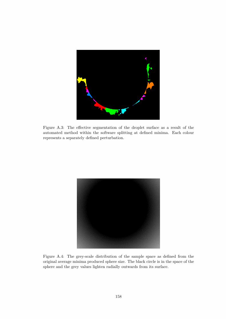
Figure A.3: The effective segmentation of the droplet surface as a result of theautomated method within the software splitting at defined minima. Each colourrepresents a separately defined perturbation.

Figure A.4: The grey-scale distribution of the sample space as defined from theoriginal average minima produced sphere size. The black circle is in the space of thesphere and the grey values lighten radially outwards from its surface.

158

Documents

warwick.ac.uk/lib-publicationswrap.warwick.ac.uk/93620/1/WRAP_Theses_Spooner_2017.pdf · 2.4 Phosphorus reaction: Thermodynamics and Kinetics . . . . . . . . . 14 ... Chapter 5 Calculating