Embed Size (px)
Citation preview
FEEDING ECOLOGY OF THE SPOTTED SEATROUT CYNOSCION NEBULOSUS IN THE EASTERN GULF OF MEXICO, WITH BEFORE AND AFTER COMPARISONS
RELATIVE TO THE DEEPWATER HORIZON OIL SPILL
By
JOHN A. ROSATI II
A THESIS PRESENTED TO THE GRADUATE SCHOOL
OF THE UNIVERSITY OF FLORIDA IN PARTIAL FULFILLMENT
OF THE REQUIREMENTS FOR THE DEGREE OF MASTER OF SCIENCE
UNIVERSITY OF FLORIDA
2017

© 2017 John A. Rosati II

To all my family and friends, especially my wife

4
ACKNOWLEDGMENTS
I would like to thank my major advisor, Dr. Debra Murie, for her guidance and
patience. Her ability to answer my questions with more questions was exceptional and,
coupled with her continual insistence to first look at the forest and then the trees, has
truly made me a better scientist. I would also like to thank my committee members, Dr.
Daryl Parkyn and Dr. Mike Allen, who were always there for encouragement, support,
and advice that extended well beyond science. I am appreciative of all my lab mates
who have helped collect samples, gave advice and solutions, and offered their
companionship even in the dark times of the ‘ginger rage’. Thanks to Mike Sipos, Geoff
Smith, and Devin Flawd for always bringing fish back when I could not. I am especially
grateful for Alicia Breton, who unexpectedly became a dear friend and was always
ready to go sampling, even if it was 4 am on the last day of a week-long trip and she did
not want to go. Thanks to Amanda Croteau and Geoff Smith for their late-night talks in
the grad carrels, without which I would still be writing my proposal. Without the help of
Paul Schueller, of FWC, I would still be struggling with data transformations in program
R. To my parents who were always supportive, thank you. Lastly, to my wife, Dory who
always empathized with me, offered encouragement, and always believed in me, I love
you.
Logistical support for this research was provided by the School of Forest
Resources and Conservation, Program of Fisheries and Aquatic Sciences, University of
Florida. Funding was provided by a grant from the Gulf of Mexico Research Initiative
and data will be made publicly available through the Gulf of Mexico Research Initiative
Information and Data Cooperative.
5
TABLE OF CONTENTS
page
ACKNOWLEDGMENTS.............................................................................................................. 4
LIST OF TABLES ......................................................................................................................... 7
LIST OF FIGURES..................................................................................................................... 10
LIST OF ABBREVIATIONS ...................................................................................................... 11
ABSTRACT ................................................................................................................................. 12
CHAPTER
1 INTRODUCTION................................................................................................................. 14
2 METHODS ........................................................................................................................... 26
Sampling Areas ................................................................................................................... 26
Fish Sampling ...................................................................................................................... 27 Feeding Chronology .................................................................................................... 28
Stomach Content Analysis ......................................................................................... 29 Diet Composition.......................................................................................................... 31 Dietary Overlap ............................................................................................................ 32
Dietary Breadth ............................................................................................................ 33 Diet Similarity Analysis................................................................................................ 34
Pre- and Post-Spill Comparison of Spotted Seatrout Diet ........................................... 35
3 RESULTS ............................................................................................................................. 39
Spotted Seatrout Sampling................................................................................................ 39
Feeding Chronology ........................................................................................................... 39 Post-Spill Contemporary Diet by Location ...................................................................... 40
Stomach Content Analysis by Location.................................................................... 40 Diet Composition in Florida ........................................................................................ 41 Diet Composition in Louisiana ................................................................................... 42
Indices of Relative Importance by Location............................................................. 43 Dietary Overlap and Breadth in Spotted Seatrout by Location ............................ 44
Similarity in the Diet of Spotted Seatrout by Location............................................ 45 Post-Spill Contemporary Diet of Spotted Seatrout by Season .................................... 47
Stomach Content Analysis by Season ..................................................................... 47
Seasonal Composition of the Diet............................................................................. 47 Indices of Relative Importance by Season .............................................................. 49
Measures of Dietary Overlap and Breadth by Season .......................................... 49 Similarity in the Diet by Season................................................................................. 50
Size-Dependent Diet of Spotted Seatrout ....................................................................... 51
6
Diet Composition by Size ........................................................................................... 51 Indices of Relative Importance by Size .................................................................... 51
Measures of Dietary Overlap and Breadth by Size ................................................ 52 Similarity in the Diet by Size....................................................................................... 53
Pre-and Post-Spill Comparison of Spotted Seatrout Diet............................................. 53
4 DISCUSSION ...................................................................................................................... 89
Feeding Chronology ........................................................................................................... 89
Contemporary Diet of Spotted Seatrout .......................................................................... 91 Pre- and Post- DWH comparison of the Spotted Seatrout Diet................................... 94
APPENDIX: WET AND DRY WEIGHTS .............................................................................. 101
LIST OF REFERENCES ......................................................................................................... 115
BIOGRAPHICAL SKETCH ..................................................................................................... 128
7
LIST OF TABLES
Table page
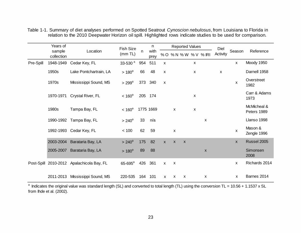
1-1 Summary of diet analyses performed on Spotted Seatrout Cynoscion
nebulosus, from Louisiana to Florida in relation to the 2010 Deepwater Horizon oil spill. Highlighted rows indicate studies to be used for comparison.... 23
2-1 Indices of digestion for fish consumed by Gag (Berens 2005) used as a proxy
for Spotted Seatrout....................................................................................................... 37
2-2 Indices of digestion for crustaceans consumed by Gag (Berens 2005) used
as a proxy for Spotted Seatrout. .................................................................................. 38
3-1 Collection locations and number of Spotted Seatrout Cynoscion nebulosus collected between 2013-2016. Sample sizes are broken down to reflect the
number of stomachs containing prey items and the percentage (%) of empty stomachs. ........................................................................................................................ 55
3-2 Regression equations used to reconstruct the whole weight of prey items consumed by Spotted Seatrout.................................................................................... 56
3-3 Diet indicies of % occurrence (%O), % numerical abundance (%N), %
reconstructed weight (%RW), and % Index of Relative Importance (%IRI) for the overall, Florida, and Louisiana diet of Spotted Seatrout. .................................. 60
3-4 Diet indices of % occurrence (%O), % numerical abundance (%N), % reconstructed weight (%RW), and Index of Relative Importance (%IRI) for the Big Bend, FL, and West Florida based diet of Spotted Seatrout............................ 63
3-5 Diet indices of % occurrence (%O), % numerical abundance (%N), % reconstructed weight (%RW), and Index of Relative Importance (%IRI) for the
Grand Isle, LA, and Venice, LA, based diet of Spotted Seatrout. .......................... 65
3-6 Diet overlap between locations measured with the Schoener’s (α) and Simplified Morisita’s (CH) indices using the reconstructed weight (RW) of
Spotted Seatrout diet. .................................................................................................... 66
3-7 Shannon-Wiener index presented as H’ and standardized as J’ calculated
using the reconstructed weight of the Spotted Seatrout diet by location and season.............................................................................................................................. 67
3-8 ANOSIM results for the diet of Spotted Seatrout based on reconstructed
weight. .............................................................................................................................. 67
3-9 SIMPER results of the Spotted Seatrout diet based on the average dietary
abundance of reconstructed weight by location ........................................................ 68
8
3-10 Total number of Spotted Seatrout collected (n) and the percentage of empty stomachs (%E) between 2013-2016 by location and season. ................................ 68
3-11 Diet indicies of % occurrence (%O), % numerical abundance (%N), % reconstructed weight (%RW), and Index of Relative Importance (%IRI) for the
temporal diet of Spotted Seatrout. ............................................................................... 69
3-12 SIMPER results for differences in the fall and spring diet of Spotted Seatrout using reconstructed weights. ........................................................................................ 72
3-13 Diet indicies of % occurrence (%O), % numerical abundance (%N), % reconstructed weight (%RW), and Index of Relative Importance (%IRI) for the
size dependent diet of Spotted Seatrout. ................................................................... 73
3-14 SIMPER results of the reconstructed diet of Spotted Seatrout diet based on size group differences. .................................................................................................. 76
3-15 Values of %DW for the diet of Spotted Seatrout in Grand Isle, LA, based on habitat type, as presented in Figure 4a of Simonsen and Cowan (2013). ............ 76
3-16 Raw comparative values of occurrence (O%), dry weight (DW%), and the redistributed DW% (r%DW) of the prey categories observed in the diet of Spotted Seatrout collected in Grand Isle, LA, before and after the DWH oil
spill between the present study, Simonsen (2008), and Russell (2005). .............. 77
3-17 Prey items in the diet of Spotted Seatrout recategorized for comparison
among the present study, Simonsen (2008), and Russell (2005). ......................... 79
3-18 Schoener’s Index (α) of overlap between the present study (Ros), Simonsen (2008) (Sim), and Russell (2005) (Rus). Overlap was measured between
overall prey groupings in bold font and finer groupings in plain font. .................... 81
A-1 Diet indicies of % wet weight (%WW) and % dry weight (%DW) and
associated Index of Relative Importance (%IRI) for the overall, Florida, and Louisiana diet of Spotted Seatrout. ........................................................................... 102
A-2 Diet indicies of % wet weight (%WW) and % dry weight (%DW) and
associated Index of Relative Importance (%IRI) for the Big Bend,FL and West Florida diets of Spotted Seatrout. .................................................................... 105
A-3 Diet indicies of % wet weight (%WW) and % dry weight (%DW) and associated Index of Relative Importance (%IRI) for the Grand Isle, LA and Venice diets of Spotted Seatrout. .............................................................................. 107
A-4 Diet indicies of % wet weight (%WW) and % dry weight (%DW) and associated Index of Relative Importance (%IRI) for the seasonal diets of
Spotted Seatrout. ......................................................................................................... 109

9
A-5 Diet indicies of % wet weight (%WW) and % dry weight (%DW) and associated Index of Relative Importance (%IRI) for the size dependent diet of
Spotted Seatrout. ......................................................................................................... 112
10
LIST OF FIGURES
Figure page
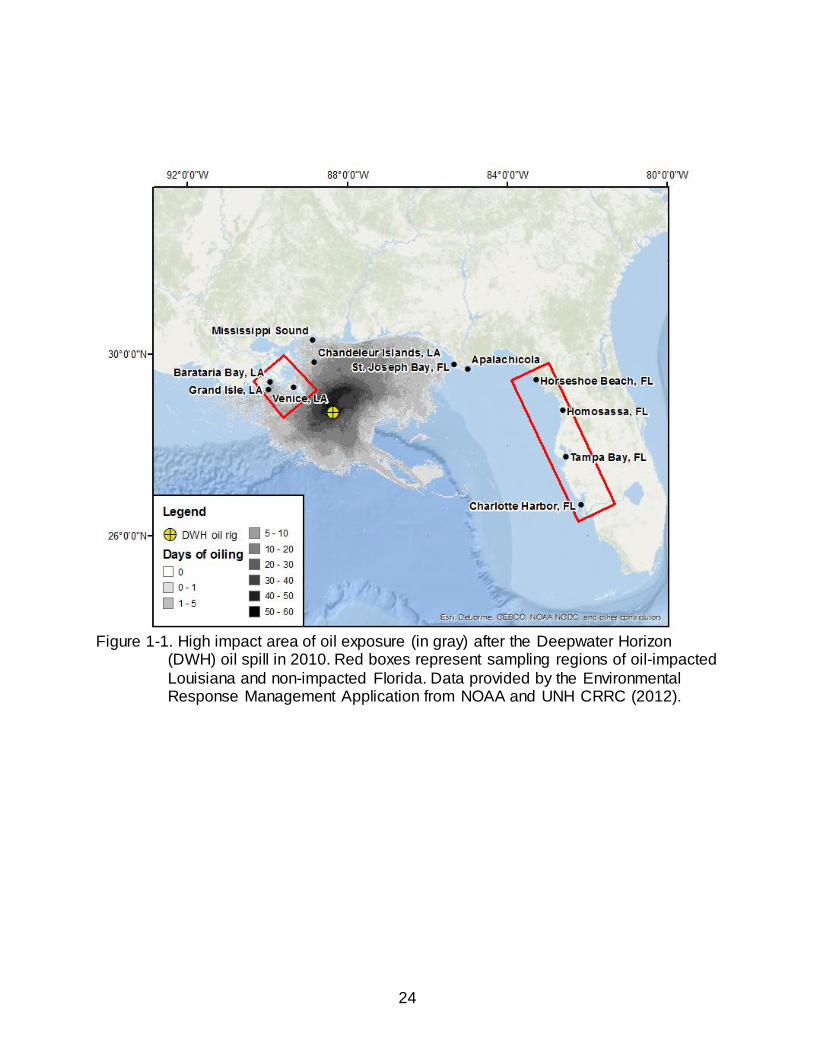
1-1 High impact area of oil exposure (in gray) after the Deepwater Horizon
(DWH) oil spill in 2010.. ................................................................................................. 24
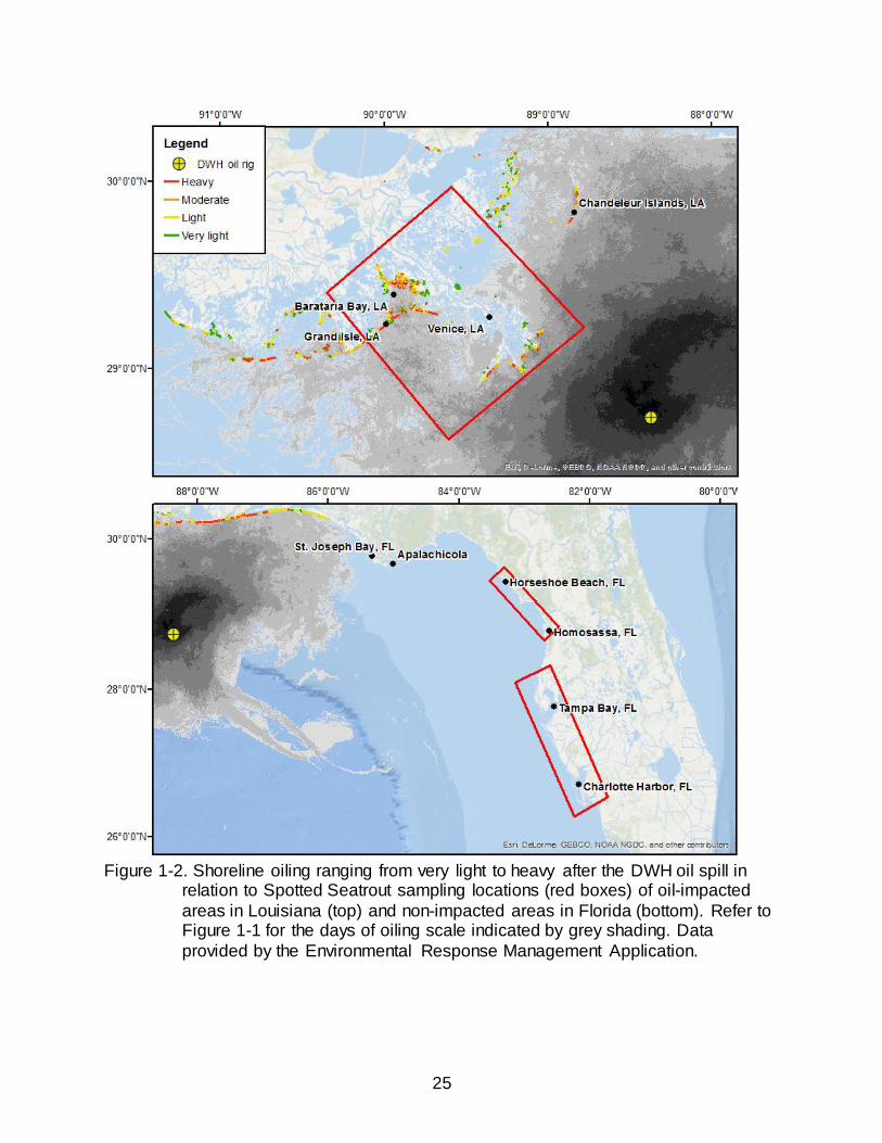
1-2 Shoreline oiling ranging from very light to heavy after the DWH oil spill in relation to Spotted Seatrout sampling locations ........................................................ 25
3-1 Length distribution of Spotted Seatrout collected between June 2013 and June 2016 for diet analysis from Florida and Louisiana after the DWH oil spill. .. 82
3-2 Percentage of Spotted Seatrout stomachs containing prey based on time of collection from Louisiana and Florida. Numbers near symbols represent the total number of stomachs collected within the time period...................................... 83
3-3 Average wet weight of prey items expressed as a percentage of Spotted Seatrout body weight based on collection time.. ....................................................... 83
3-4 Frequency of digestion code occurrence based on collection time for prey items occurring in the stomachs of Spotted Seatrout............................................... 84
3-5 Prey accumulation curves for the overall and location-based diet of Spotted
Seatrout.. ......................................................................................................................... 85
3-6 Top - MDS plot portraying similarity of the Spotted Seatrout diet between
collection locations. ........................................................................................................ 86
3-7 Top - MDS plot portraying similarity of diet in Spotted Seatrout between collection season. ........................................................................................................... 87
3-8 Top - MDS plot portraying similarity of diet in Spotted Seatrout between body size. .................................................................................................................................. 88
11
LIST OF ABBREVIATIONS
ANOSIM Analysis of Similarity
ANOVA Analysis of Variance
CL Carapace length
CW Carapace width
DW Dry weight
DWH Deepwater Horizon
FL Florida
GOM Gulf of Mexico
IRI Index of Relative Importance
LA Louisiana
MDS Multidimensional Scaling
MTL Maximum total length
NMFS National Marine Fisheries Service
PAHs Polycyclic Aromatic Hydrocarbons
PWS Prince William Sound
RW Reconstructed weight
SIMPER Similarity Percentage
SL Standard length
TL Total length
VCL Vertebral column length
WW Wet weight
12
Abstract of Thesis Presented to the Graduate School of the University of Florida in Partial Fulfillment of the
Requirements for the Master of Science
FEEDING ECOLOGY OF THE SPOTTED SEATROUT CYNOSCION NEBULOSUS IN THE EASTERN GULF OF MEXICO, WITH BEFORE AND AFTER COMPARISONS
RELATIVE TO THE DEEPWATER HORIZON OIL SPILL
By
John A. Rosati II
August 2017
Chair: Debra Murie
Cochair: Daryl Parkyn Major: Fisheries and Aquatic Sciences
This study investigated the feeding ecology of adult Spotted Seatrout Cynoscion
nebulosus, an estuarine-dependent predator and commonly caught recreational fish
species, and assessed possible changes before and after the Deep Water Horizon oil
spill in 2010. To compare the pre-spill diet data with present day data, a post-spill
baseline diet was first developed for Spotted Seatrout collected from oiled regions in
Louisiana and non-oiled regions in Florida. Stomachs were collected between 2013-
2016 from two impacted areas in Louisiana, Barataria Bay (Grand Isle) (n=287) and
Venice (n=149), and two control regions in Florida, the Big Bend region (n=211) and the
West-Central region (n=256).
Assessment of post-spill feeding chronology based on frequency of empty
stomachs, stomach content weight (expressed as percentage of wet body weight), and
prey digestion codes as a function of time (0600-2000 h) confirmed a period of peak
feeding in the early to mid-morning (0800-1000 h). The post-spill diet was described as
a function of location, season, and size (mm TL) utilizing the percentages of occurrence
(%O), numerical abundance (%N), and reconstructed whole weight of prey items
13
(%RW). Differences in diet were detected between seasons (spring and fall) and size
groups. The %O, %N, and %RW of penaeid shrimp peaked in the spring diet and
gradually declined into the fall, whereas the reverse was true of clupeids and engraulids
(Anchoa spp.). Size-dependent differences were detected among the smallest Spotted
Seatrout (150-300 mm TL), which consumed greater amounts engraulids, and the
largest adult Spotted Seatrout (>350 mm TL), which consumed greater amounts of
sciaenids and Pinfish Lagodon rhomboides. Diet overlap based on Schoener’s Index
and the Simplified Morisita’s Index, analysis of similarity (ANOSIM), and multi-
dimensional scaling (MDS) indicated that the post-spill diet of Spotted Seatrout in
Barataria Bay, LA, Big Bend, FL, and West Florida were most similar.
Direct comparison of the pre- and post-spill diet of Spotted Seatrout in Barataria
Bay, LA, was limited to two pre-spill diet studies from Barataria Bay with relatively low
resolution of prey identification. This comparison revealed, however, that the post-spill
diet was more similar to one of the pre-spill diet studies when compared to the similarity
between the two pre-spill diet studies alone. This suggests a large natural variation in
the diet of Spotted Seatrout and indicated that any change in the post-spill diet could not
necessarily be ascribed to impacts from the Deepwater Horizon oil spill.
14
CHAPTER 1 INTRODUCTION
The Deepwater Horizon (DWH) oil spill is considered the worst environmental
disaster in the history of the United States and the second largest oil spill worldwide
(Levy and Gopalakrishnan 2010; Carriger and Barron 2011; Graham et al. 2011). From
20 April to 15 July 2010, an estimated 4.9 million barrels of crude oil was released into
the Gulf of Mexico (GOM) (McNutt et al. 2011, 2012). Oil spanned four states:
Louisiana, Mississippi, Alabama, and northwestern Florida, leaving the Texas coast and
Florida’s west coast relatively untouched (Figure 1-1). Survey crews monitored 7,058
km of shoreline of which 1,773 km were reported oiled to varying degrees. Across the
four states, beach and marsh habitats encompassed 51% and 45% of the total reported
oiled shorelines, respectively. Louisiana was most heavily affected and accounted for
approximately 60% of the reported oiled shorelines and 95% of the oiled marsh habitat.
Past oil spills, such as the Exxon-Valdez in Prince William Sound (PWS), Alaska
(Bragg et al. 1994), the barge Florida in Massachusetts (Teal and Howarth 1984), and
the tanker Arrow in Nova Scotia (Scarratt and Zitko 1972), have given scientists
opportunities to study the effects of crude oil and petroleum products in coastal
ecosystems. Peterson et al. (2003) reviewed literature from these past oil spills and
determined that ecosystems are influenced by the short and long term impacts of oil
exposure. The short term effect of acute mortality to biological organisms is often
predictable, whereas the long term effects to organisms from sub-lethal acute and
chronic oil exposure often arise years later, are difficult to predict, and lead to direct and
indirect effects. After the Exxon Valdez, Pink Salmon Oncorhynchus gorbuscha eggs
experienced decreased survival for up to 4 years after the spill due to increased levels
15
of polycyclic aromatic hydrocarbons (PAHs) in spawning streams (Bue et al. 1998).
Furthermore, continuous exposure to sub-lethal concentrations of oil can compromise
health, reproduction, and growth leading to delayed responses among populations. Pink
Salmon fry grew slower following the Exxon-Valdez oil spill, which increased size-
dependent predation (Rice et al. 2001). Adult Pink Salmon, exposed to oil as fry during
a controlled laboratory experiment and then released, were reproductively less
successful because of deformities among their embryos (Heintz et al. 1999).
After the DWH oil spill, varying degrees of oil exposure throughout the northern
GOM created a hot spot for many ecological studies, particularly in Barataria Bay, LA,
where oil exposure was relatively high (Figure 1-2). Fodrie et al. (2014) reviewed
delayed impacts from the DWH oil spill specific to fisheries and categorized five direct
effects, each having implications for larger, more complicated, indirect effects. Direct
effects discussed by Fodrie et al. (2014) included physiological and developmental
issues (Whitehead et al. 2011; Dubansky et al. 2013; Incardona et al. 2014; Pilcher et
al. 2014), mortality (McCall and Pennings 2012), habitat loss (Lin and Mendelssohn
2012; Silliman et al. 2012), potential decreases to primary production and nutrient flow,
and lastly, fishery closures. These direct effects have led to indirect effects at the
population and community levels, and have been correlated with diet shifts (Tarnecki
and Patterson 2015; Norberg 2015) and decreases in somatic and reproductive growth
(Flawd 2015; Herdter et al. 2017) of important commercial and recreational fish species.
Changes in diet and growth rates can alter the predictability of fish growth and
reproduction, which are critical to fisheries management (Walters and Martell 2004),
and are dependent on available energy acquired from diet and consumption (Richter
16
1999). Changes in diet could therefore influence fish productivity and result in
necessary management changes. Diet changes generally occur due to shifts in prey
availability, increased energy demands related to size and reproduction, or to limit
competition for resources (Winemiller 1989; Bergman and Greenberg 1994; Mol 1995;
Eggleston et al. 1998; McCormick 1998; Persson and Hansson 1999; Renones et al.
2002; Galarowicz et al. 2006). Anthropogenic effects such as fishing and pollution, or
environmental effects such as temperature variability, can also lead to variation in diet
(Olson 1996; Alonso et al. 2002; Link and Garrison 2002; Pazzia et al. 2002; Stetter et
al. 2005). These effects directly impact prey sources, which then indirectly affect
predators due to an alteration of prey availability. Most recently, Tarnecki and Patterson
(2015) linked decreases in the abundance of zooplankton in the months following the
DWH oil spill to a trophic level shift of Red Snapper Lutjanus campechanus. Stomach
content analysis indicated an increase of higher trophic level prey following the DWH oil
spill and a decrease in the consumption of zooplankton, which was confirmed by stable
isotope analysis. It is possible that diet shifts seen in Red Snapper could have also
occurred in other recreational and commercial important fishes in oil-stricken habitats of
Louisiana.
The Spotted Seatrout Cynoscion nebulosus is a common estuarine fish species
throughout the coastal waters of the GOM, and is one of the most popular species for
recreational inshore fishing. Average recreational catch of Spotted Seatrout from 2003
to 2012 was estimated at 31 million fish per year. In 2012, anglers caught an estimated
33 million Spotted Seatrout throughout the GOM, with nearly 50% caught in coastal
waters of Louisiana (NMFS 2014).
17
Spotted Seatrout are rather unique in that they are essentially non-migratory;
tagging studies have found that few individuals travel further than 30 km from their
tagging location (Iversen and Tabb 1962; Adkins et al. 1979; Baker Jr and Matlock
1993; Hendon et al. 2002; Walters et al. 2009). The lack of migration has created
estuarine-specific population dynamics throughout the GOM. The most commonly
observed differences in populations among estuaries are growth rates and size at
maturity (Iversen and Tabb 1962; Hein and Shepard 1979; Overstreet 1983; Brown and
Arnolos 1988; Wieting 1989; Murphy and Taylor 1994; Brown-Peterson and Warren
2001; Brown-Peterson et al. 2002; Nieland et al. 2002; Bedee et al. 2003; Johnson et al.
2011).
The diet of Spotted Seatrout has been studied to various degrees throughout the
GOM, with many studies occurring prior to 2000, 10 years before the DWH oil spill
(Table 1-1). Methodology among studies has varied greatly, which has resulted in
disagreements of prey resource utilization among adults, particularly between season
and location, and has made comparisons difficult. Many previous studies have focused
on juvenile (<200 mm standard length, SL) Spotted Seatrout and only a few recent
studies have quantitatively assessed the diet of adults. Spotted Seatrout have been
previously described as an opportunistic carnivore that mainly targets fish and
crustaceans (Pearson 1929; Gunter 1945; Miles 1950; Tabb 1966; Carr and Adams
1973; Adkins et al. 1979; Perret et al. 1980; Overstreet 1983; Murphy and Taylor 1994;
Llanso et al. 1998). Fish size, season, and habitat type have been linked to differences
in the chief components of the Spotted Seatrout diet (Gunter 1945; Houde and Lovda
18
1984; Hettler Jr 1989; McMichael and Peters 1989; Mason and Zengel 1996; Richards
2014).
Spotted Seatrout larvae (<15 mm SL) mainly feed on invertebrates, such as
copepods, larval bivalves, and gastropods (McMichael and Peters 1989). Juveniles (15-
30 mm SL) consume larger copepods, amphipods, mysids, and small fish (McMichael
and Peters 1989; Mason and Zengel 1996). Juveniles approximately 60 mm total length
(TL) shift away from small shrimp, copepods, and amphipods and rely more on small
fish and shrimp (Mason and Zengel 1996). Adult Spotted Seatrout (>200 mm SL) feed
primarily on shrimp and fish (Darnell 1958; Tabb 1966; Overstreet 1983; Mason and
Zengel 1996; Llanso et al. 1998; Richards 2014) but the importance of invertebrates,
specifically penaeid shrimp, has been debatable (Darnell 1958; McMichael and Peters
1989). Pearson (1929) and Gunter (1945) reported that shrimp occurred in 61% and
35% of stomachs from adult Spotted Seatrout, respectively, however Gunter noted most
of his fish were sampled in winter months. Furthermore, fish occurred more frequently in
the diet than shrimp in Spotted Seatrout >350 mm SL (Moody 1950; Darnell 1958).
More recent information on the diet of adult Spotted Seatrout in the Gulf of
Mexico, but still prior to the DWH oil spill, was limited to two studies done in Barataria
Bay, LA, including Russell (2005) with samples collected in 2003-2004 and Simonsen
(2008) with samples collected in 2005-2007 (Table 1-1). Prey resource categories used
by Seatrout in each of these studies were similar, however, the contribution of those
prey types by occurrence and dry weight varied greatly. The diet of adult Spotted
Seatrout in both studies was dominated by various fishes followed by penaeid shrimp.
Seasonally, although each study observed increased values of penaeid shrimp during
19
the spring, they found no statistical difference among seasons. In addition, neither study
found significant differences between the diet of fish collected from various habitat types
such as mud, marsh edge, or artificial reefs within the bay. Russell (2005) also tested
for variation in diet among size groups of adult fish but found no difference. Both of
these studies therefore supported earlier studies that categorized Spotted Seatrout as a
generalist carnivore with a variable diet in relation to its size and season of capture.
Adult Spotted Seatrout diet information collected in the GOM after the DWH oil
spill was also limited to two studies, but neither study was done in oil-impacted
Barataria Bay where pre-spill diet information was available from Russell (2005) and
Simonsen (2008). Barnes (2014) collected Spotted Seatrout in 2011-2013 from the
Mississippi Sound, a region that experienced moderate oiling (Figure 1-1), however he
did not compare diets between his study and the two pre-spill studies. While the
resolution of identified prey types was generally low, Barnes observed a significant
increase in occurrence of fish in the summer diet of Spotted Seatrout compared to the
spring. Richards (2014) studied the diet of Spotted Seatrout in 2010-2012 from
Apalachicola Bay, FL, a region not impacted by the DWH oil spill, and to my knowledge
is the most recent and thorough diet study of adult Spotted Seatrout. Richards’ stomach
content analysis identified diet differences between locations within Apalachicola Bay
but not season. However, like the findings of Russell (2005) and Simonsen (2008),
Richards also observed a general increase in the amount of shrimp during the spring
season followed by a reliance on fishes during the rest of year. Contrary to the findings
of Russell (2005), Richards (2014) identified differences in diet among fish size with
20
larger adult Spotted Seatrout consuming increased amounts of fish while smaller fish
<200 mm SL consumed more shrimp.
While various studies have drawn different conclusions of the prey resource
utilization in the spatial, temporal, and size-related diet of Spotted Seatrout, it was clear
that there was an important trophic linkage between shrimp, small fishes, and Spotted
Seatrout. Changes with the availability of prey fish and shrimp could therefore influence
the diet and overall productivity of Spotted Seatrout populations. Studying trophic
dynamics, predator prey interactions, and biological consequences of ecosystem
alterations has become increasingly important in fisheries management. Advances in
the understanding of ecosystem interdependence have led researchers toward
ecosystem-based management that uses trophic linkages to analyze the interaction
between the ecological and anthropogenic effects on sustainability (Fulton et al. 2011).
This management style is often beneficial but relies on highly detailed and accurate
data regarding the trophic dynamics and predator prey interactions within a system
(Pauly et al. 2000; Latour et al. 2003). Managers and conservationists need a thorough
understanding of the trophic dynamics of an ecosystem to provide proper management
decisions (Christensen and Walters 2004). Environmental disturbances, such as the
DWH oil spill, can disrupt trophic dynamics within an ecosystem, and therefore the diets
of organisms are important to monitor before and after environmental changes to detect
potential diet shifts that can ultimately affect productivity.
The scientific community has become aware of deficiencies in and need for
quality baseline data to assess the effects of disturbances and evaluate restoration
efforts, particularly when considering ecological disasters (Kennedy and Cheong 2013).
21
Studies assessing the ecological impacts of the DHW oil spill have had limited pre-spill
data available to draw on for post-spill comparisons, with many studies having only a
single pre-spill indicator (i.e., data point) to compare with any potential post-spill
changes. This becomes problematic because if there is no estimate of the natural
annual variability in the system in the pre-spill period, it then makes it mostly impossible
to determine if there was actually an impact due to the perturbation or simply a change
that was within the natural annual variability of the system overall. Comparatively, the
diet of Spotted Seatrout has been relatively well documented and there are two studies
that occurred in the years prior to the DWH oil spill, specifically in Barataria Bay. It was
therefore an opportune time to collect contemporary data on the diet of Spotted
Seatrout from Barataria Bay and compare it to the diet information from the pre-spill
studies to determine if there had been a detectable post-spill change in the diet of
Spotted Seatrout.
The first major goal of this project was to determine the contemporary diet of
Spotted Seatrout in estuarine waters of southeastern Louisiana, which was impacted as
a result of the DWH oil spill, compared to Seatrout from estuarine waters of western
Florida, which as a reference region had no oil impact from the DWH spill. This diet
analysis was necessary to estimate the natural variability in the contemporary diet of
Spotted Seatrout among estuaries within and outside of the overall impacted area of the
northern GOM (Figure 1-1) on an estuary-specific, season-specific, and size-specific
basis. These factors have previously been reported to affect the diet of Spotted
Seatrout to varying degrees. The second major goal of this project was to then compare
the contemporary post-spill diet of Spotted Seatrout in Louisiana, and Barataria Bay

22
specifically, with the pre-spill diet analyses from Barataria Bay by Russell (2005) and
Simonsen (2008) to detect potential changes in the baseline diet of Spotted Seatrout in
an estuary known to be impacted by the DWH oil spill.
23
Table 1-1. Summary of diet analyses performed on Spotted Seatrout Cynoscion nebulosus, from Louisiana to Florida in relation to the 2010 Deepwater Horizon oil spill. Highlighted rows indicate studies to be used for comparison.
% O
Pre-Spill 1948-1949 Cedar Key, FL 33-530 a 954 511 x
1950s Lake Pontchartrain, LA > 180a 66 48 x
1970s Mississippi Sound, MS > 299a 373 340 x
1970-1971 Crystal River, FL < 160a 205 174
1980s Tampa Bay, FL < 160a 1775 1669
1990-1992 Tampa Bay, FL > 240a 33 n/a
1992-1993 Cedar Key, FL < 100 62 59
2003-2004 Barataria Bay, LA > 240a 175 82 x
2005-2007 Barataria Bay, LA > 180a 89 88
Post-Spill 2010-2012 Apalachicola Bay, FL 65-695a 426 361 x
2011-2013 Mississippi Sound, MS 220-535 164 101 x
x x Darnell 1958
x x
xCarr & Adams
1973
x
x Llanso 1998
x x
Mason &
Zengle 1996
x x x Russel 2005
x x
x Richards 2014
x
a Indicates the original value was standard length (SL) and converted to total length (TL) using the conversion TL = 10.56 + 1.1537 x SL
from Ihde et al. (2002).
Barnes 2014
% IRI% V% W% N
x x x x
Simonsen
2008
x
Reported ValuesDiel
ActivitySeason Reference
McMicheal &
Peters 1989
Overstreet
1982
Moody 1950
Years of
sample
collection
LocationFish Size
(mm TL)n
n
with
prey
24
Figure 1-1. High impact area of oil exposure (in gray) after the Deepwater Horizon
(DWH) oil spill in 2010. Red boxes represent sampling regions of oil-impacted
Louisiana and non-impacted Florida. Data provided by the Environmental Response Management Application from NOAA and UNH CRRC (2012).
25
Figure 1-2. Shoreline oiling ranging from very light to heavy after the DWH oil spill in
relation to Spotted Seatrout sampling locations (red boxes) of oil-impacted
areas in Louisiana (top) and non-impacted areas in Florida (bottom). Refer to Figure 1-1 for the days of oiling scale indicated by grey shading. Data
provided by the Environmental Response Management Application.
26
CHAPTER 2 METHODS
Sampling Areas
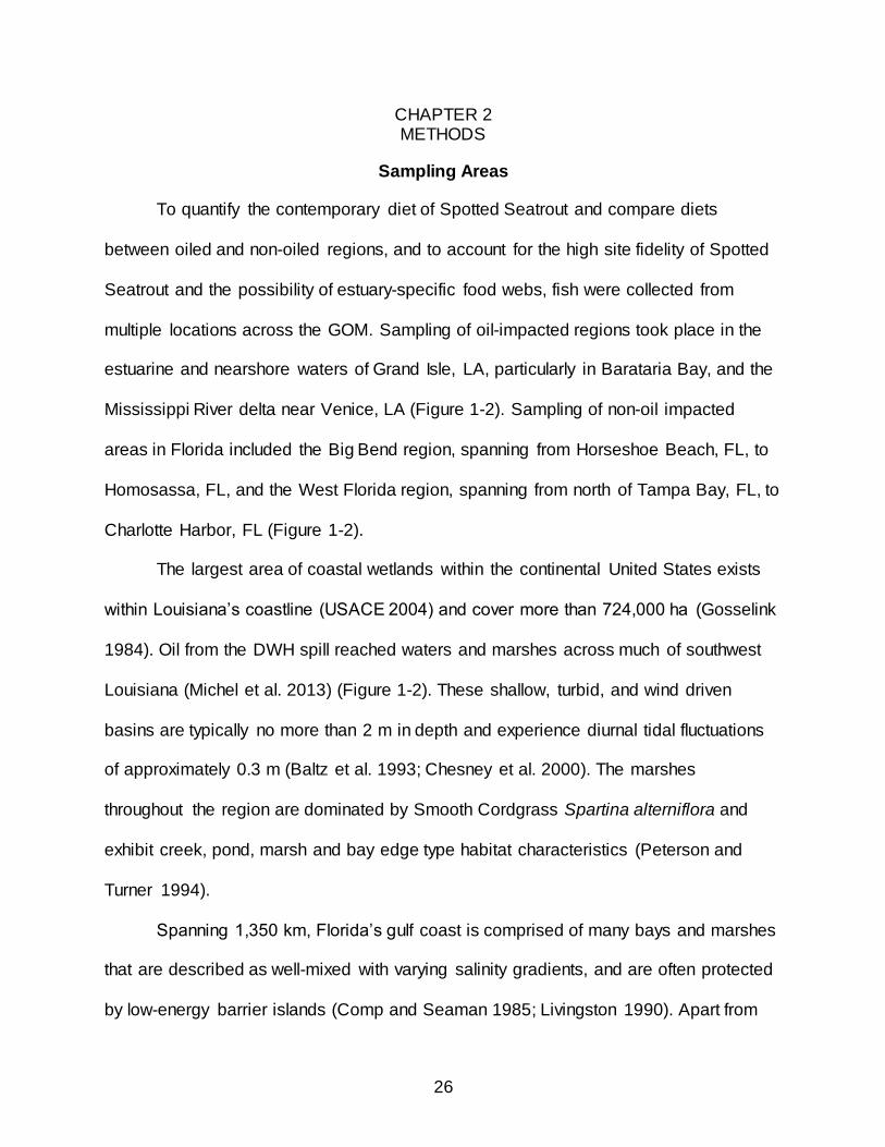
To quantify the contemporary diet of Spotted Seatrout and compare diets
between oiled and non-oiled regions, and to account for the high site fidelity of Spotted
Seatrout and the possibility of estuary-specific food webs, fish were collected from
multiple locations across the GOM. Sampling of oil-impacted regions took place in the
estuarine and nearshore waters of Grand Isle, LA, particularly in Barataria Bay, and the
Mississippi River delta near Venice, LA (Figure 1-2). Sampling of non-oil impacted
areas in Florida included the Big Bend region, spanning from Horseshoe Beach, FL, to
Homosassa, FL, and the West Florida region, spanning from north of Tampa Bay, FL, to
Charlotte Harbor, FL (Figure 1-2).
The largest area of coastal wetlands within the continental United States exists
within Louisiana’s coastline (USACE 2004) and cover more than 724,000 ha (Gosselink
1984). Oil from the DWH spill reached waters and marshes across much of southwest
Louisiana (Michel et al. 2013) (Figure 1-2). These shallow, turbid, and wind driven
basins are typically no more than 2 m in depth and experience diurnal tidal fluctuations
of approximately 0.3 m (Baltz et al. 1993; Chesney et al. 2000). The marshes
throughout the region are dominated by Smooth Cordgrass Spartina alterniflora and
exhibit creek, pond, marsh and bay edge type habitat characteristics (Peterson and
Turner 1994).
Spanning 1,350 km, Florida’s gulf coast is comprised of many bays and marshes
that are described as well-mixed with varying salinity gradients, and are often protected
by low-energy barrier islands (Comp and Seaman 1985; Livingston 1990). Apart from
27
heavy oil deposition near the Alabama-Florida border in May of 2010 immediately after
the DWH well blowout, impact was deemed very light to none from St. Josephs Bay, FL,
and eastward (Michel et al. 2013) (Figure 1-2).
Bay and estuary systems of Florida’s gulf coast are highly variable in physical
characteristics relative to the marsh basins in southern Louisiana. East of Apalachicola
Bay to Homosassa, FL, is an open water region with few enclosures or barrier islands,
known as the Big Bend (Figure 1-2). Freshwater discharge from numerous rivers,
creeks, and springs meets the GOM and forms an open estuary environment with
typical flora and fauna. Barrier islands return to protect embayments just north of Tampa
Bay and scattered mangrove stands begin to emerge among the dominate salt marsh.
Tampa Bay (Figure 1-2) is influenced by five major rivers but freely circulating GOM
water maintains a strong halocline. Seagrasses and mangroves dominate the shoreline
of Tampa Bay. Charlotte Harbor (Figure 1-2) is less developed compared to Tampa
Bay, and much of the shoreline is unperturbed and seagrasses cover approximately
30% of the bottom substrate (Comp and Seaman 1985; Tomasko et al. 2005).
Fish Sampling
Spotted Seatrout were collected via rod and reel. Bait type, catch time, and
location were recorded for captured fish. Fish were kept on ice until necropsied in the
laboratory. Maximum total length (MTL) (±1 mm), wet weight (±0.1 g), and sex were
recorded. Stomachs were excised and, at that point in time, the mouth and esophagus
was visually inspected for regurgitated stomach contents. Stomachs and all contents
were bagged and labeled accordingly and then frozen until analyzed. Sagittal otoliths
28
were collected, cleaned, and stored dry in vials for growth analysis associated with an
ongoing study.
Feeding Chronology
Patterns of feeding chronology were addressed by using stomach content
weight, digestion percentages of prey items, and the percentage of empty stomachs, all
as a function of collection time. Stomachs were grouped into 2-h time periods ranging
from 0600-2000 h. Samples collected between 2000-2400 h were excluded from all
feeding chronology analysis due to low sample size (n=3).
Continuity and intensity of feeding was assessed by comparing the mean wet
weight of stomach contents, expressed on a percent bodyweight basis, collected from
time groups. Analysis of variance (ANOVA) was used with post-hoc tests to determine if
means differed among time groups (Cortes 1997).
Cortes (1997) suggests that stomach content weight alone is not a sufficient
measure of feeding continuity; it is merely an indication of feeding intensity and
chronology, therefore digestion stages and empty stomachs within a sample were also
considered. Digestion codes were based on those developed for Gag Mycteroperca
microlepis by Berens (2005) (Tables 2-1 and 2-2). Prey items were assigned to one of
the following categories representing a range in digestion percentage: 0 (<5%), 1 (5-
25%), 2 (25-50%), 3 (50-75%), 4 (75-90%), and 5 (>90%). A separate descriptive index
for fish (Table 2-1) and crustaceans (Table 2-2) was used. A contingency table was
used to test for significant differences between frequency of digestion codes and
collection times (Krebs 1999).
The percentage of empty stomachs from Spotted Seatrout was calculated as:
29
%𝐸𝑚𝑝𝑡𝑦 =# 𝑜𝑓 𝑒𝑚𝑝𝑡𝑦 𝑠𝑡𝑜𝑚𝑎𝑐ℎ𝑠
𝑡𝑜𝑡𝑎𝑙 # 𝑜𝑓 𝑠𝑡𝑜𝑚𝑎𝑐ℎ×100 (2-1)
Differences in the frequency of empty and non-empty stomachs collected among
time blocks was tested using a contingency table (Krebs 1999).
Stomach Content Analysis
During stomach content analysis, stomachs were thawed, cut open, and rinsed
over a collecting dish to extract all contents. Once sorted, whole and partial prey items
were assigned a reference number and then counted, damp blotted, and weighed (wet
weight, WW) (± 0.0001 g). Length measurements (± 0.01 mm) were also taken,
including total length (TL), standard length (SL), vertebral column length (VCL, back of
skull to the hypural plate), carapace length (CL, for shrimp, from the back of the eye
socket to the posterior edge of the carapace), and carapace width (CW, for crabs,
measured as the maximum width of the carapace). These length measurements were
then used in regression analysis to reconstruct the weight of any digested prey items to
their undigested whole weight (reconstructed weight, RW). Remaining mucus and liquid
in the collecting dish were transferred to a 500 mL beaker. A gravity sieve was created
by a small flow of water into the beaker in which light material, such as mucus flowed
out of the top while more dense items, such as otoliths, remained at the bottom (Murie
and Lavigne 1985). Collected otoliths were rinsed, dried, photographed, and measured
for otolith length and height and were compared to field-collected specimens and photo
references (Baremore and Bethea 2010) for identification.
Once all prey items were identified to the lowest possible taxonomic level using
relevant identification keys (Abele and Kim 1986; Carpenter 2002; Kells and Carpenter
30
2011; Bowling 2012), dry weights were measured to allow comparisons to indices in
previous studies that used only dry weight. To measure dry weight (DW), unique prey
items within each stomach were placed in pre-weighed aluminum pans and weighed
(±0.0001 g). Prey items that occurred more than once in a single stomach were pooled
and weighed. Weighing pans were then placed in a drying oven at 60 C for 24 h or unti l
a constant weight was achieved. After drying, pans were allowed to cool to room
temperature in a desiccator and were then re-weighed. Dry weight of prey items was
then determined by subtracting the pan weight from the total dried weight.
Regressions of whole prey size or weight as a function of partial prey
measurements and otolith measurements were used to reconstruct the original weight
of whole prey items (Murie 1995). Whole prey were opportunistically sampled from
Cedar Key, FL, and Grand Isle, LA, for use in regression analysis and as reference
specimens for prey identification. Regressions based on using otolith length to estimate
whole prey weight were prioritized for prey fish. Measures of SL, TL, or VCL were used
if otolith length was not available. Using the SL of fishes was often prioritized as the soft
rays of the caudal fin were quick to digest causing measures of TL to be unreliable.
Regressions for crustaceans were based on carapace length (CL) and carapace width
(CW). If regressions were not available for a prey item, a regression from a similar prey
item, based on taxonomy, shape, and relative size was used. If no measurements were
available, prey items were assigned an average weight that best reflected the estimated
size of that prey item. Parasitic isopods in the family Cymothidae were included as prey
items in this study because their presence was associated with clupeids and they were
observed inside the mouths of consumed Gulf Menhaden Brevoortia patronus.
31
Diet Composition
To ensure that enough stomachs were sampled to adequately describe the diet
of Spotted Seatrout, cumulative prey curves were generated post-hoc (Ferry and Cailliet
1996). This curve plots the total number of stomachs against the mean number of new
prey items found in each stomach. If the curve approached an asymptote (i.e. within the
last 10 stomachs the number of new prey items increased by less than 5%), then a
satisfactory amount of stomachs had been analyzed to say the diet was well described
(Ferry and Cailliet 1996; Cortes 1997; Baremore 2007). Individual stomachs and their
associated prey items were randomized and cumulative prey curves were generated
using the Vegan package (Oksanen et al. 2010) found in the statistical software of
program R (R Development Core Team 2010).
Diet composition was analyzed using three metrics: frequency of occurrence
(%O), numerical abundance (%N), and reconstructed weight (%RW) (Hyslop 1980;
Cortes 1997). The RW of prey items was used to limit the effects of digestion and the
bias associated with partially digested prey weight. Diet composition using prey wet
weight (%WW) and dry weight (%DW) was included for comparative purposes to benefit
future diet studies (Appendix A). Occurrence is the number of stomachs containing a
specific prey item divided by all non-empty stomachs, %N is the total number of one
prey type divided by the total number of prey items in all stomachs, and %W is the
pooled weight of one prey type from all stomachs divided by the total weight of all prey
items using each of the previously described weight measurements. An Index of
Relative Importance (IRI) (Pinkas 1971) for primary categories of prey resources was
calculated as
𝐼𝑅𝐼 = (%𝑁 + %𝑊) × %𝑂 (2-2)
32
The IRI was expressed as a percentage based upon the IRI for each prey category over
the sum of all IRI values using (Cortes 1997):
% 𝐼𝑅𝐼 = 𝐼𝑅𝐼 𝑓𝑜𝑟 𝑒𝑎𝑐ℎ 𝑝𝑟𝑒𝑦 𝑐𝑎𝑡𝑒𝑔𝑜𝑟𝑦
𝑆𝑢𝑚 𝑜𝑓 𝑎𝑙𝑙 𝐼𝑅𝐼 𝑣𝑎𝑙𝑢𝑒𝑠 ×100 (2-3)
All metrics of diet composition were analyzed for location, season, and size.
Seasons were defined as spring (March, April, May), summer (June, July, August), fall
(September, October, November), and winter (December, January, February). Based
on TL, and to support evenness among sample sizes, Spotted Seatrout were divided
into three size groups: 1 (150-299 mm), 2 (300-349 mm), 3 (350-600 mm).
Dietary Overlap
Measures of diet overlap are useful to identify the level of diet similarity between
and within species, seasons, and habitat type (Krebs 1999; Garvey and Chipps 2013).
The diet of Spotted Seatrout collected from the sampling areas was measured for
overlap using Schoener’s Index and the Simplified Morista’s Index of similarity based on
the values of reconstructed weight. Schoener’s Index is also known as the percentage
overlap (Krebs 1999) and is one of the most common and easily interpreted indices.
The simplified Morisita Index is more commonly used as opposed to Schoener’s Index
because it exhibits less bias as the number of resource categories increases (Smith and
Zaret 1982; Krebs 1999). Each overlap index was calculated using values from the
taxonomic resolution of family due to digestion, which allowed for consistent
identification to this level. For each measure, values of overlap greater than 0.6 were
considered biologically significant (Zaret and Rand 1971; Mathur 1977; Wallace 1981).
Schoener’s Index (∝) was calculated as it was reported by Wallace (1981):
33
∝= 1 − 0.5(∑ |𝑝𝑖𝑥 − 𝑝𝑖𝑦|)𝑖=1,𝑛 (2-4)
where ∝ ranges from 0 (no overlap) to 1 (complete overlap), 𝑝𝑖𝑥 is the proportion of prey
i in the diet of fish from location x, and 𝑝𝑖𝑦 is the proportion of prey i in the diet of fish
from location y. The Simplified Morisita Index (CH) was calculated as:
𝐶𝐻 =2 ∑ 𝑝𝑖𝑥𝑝𝑖𝑦
𝑛𝑖
∑ 𝑝𝑖𝑥2 +𝑛
𝑖∑ 𝑝𝑖𝑦
2𝑛𝑖
(2-5)
where pix is the proportion of resource i in respect to all resources used by fish from
location x, and piy is the proportion of resource i in respect to all resources used by fish
from location y, and n is the total number of resource categories (Horn 1966; Krebs
1999).
Dietary Breadth
The diet was further analyzed to determine if Spotted Seatrout are generalists or
specialists by using measures of niche breadth, such as the Shannon-Wiener measure
(H’), to quantitatively assess the range of prey items (Krebs 1999):
𝐻 ′ = − ∑ 𝑝𝑗 log 𝑝𝑗 (2-6)
where pj is the proportion of individuals using prey type j. An issue with the Shannon-
Wiener measure is that H’ ranges from 0 to ∞, which is adequate for relative
comparisons but makes comparisons among studies difficult to put into perspective,
especially if there are differences among the number of prey types. Values of H’ were
calculated utilizing the RW of prey items and were then standardized on a scale from 0
34
(narrow niche breadth) to 1 (broad niche breadth) by using the evenness measure J’:
𝐽′ =𝐻′
log 𝑛 (2-7)
where n is to total number of resource states.
Diet Similarity Analysis
Similarity within diet composition using RW was assessed using analysis of
similarity (ANOSIM) and similarity percentages (SIMPER) and then visualized with
multi-dimensional scaling (MDS) in the multivariate statistics package PRIMER v6
(Clarke and Gorley 2006). As with the measures of dietary overlap and breadth,
similarity in the diet was assessed at the family level of prey identification, which
because of prey digestion was a comparable level among most prey types. Diet
composition using the RW at the family taxonomic level of prey categories for each
individual stomach was imported into PRIMER. Weights were transformed into percent
composition for individual stomachs and were then square root transformed to
downweigh the contributions of quantitatively dominant species (Clarke and Warwick
2001). A resemblance matrix comparing individual stomachs was creating using Bray-
Curtis similarity coefficients. ANOSIM uses a permutation test to statistically analyze the
resemblance matrix and produce a global R statistic assessing dissimilarity within and
among samples. The R statistic ranges from 0 (complete similarity) to 1 (complete
dissimilarity). Observed R values are compared to the expected R value to determine if
dissimilarities exist. The number of possible permutations and consequently statistical
power quickly becomes very large (for example, 10 replicates of 4 sample locations
becomes 5.36e+32 permutations), therefore, significance in the ANOSIM is set at 0.001
35
or 0.1%. If significance was detected, a post-ANOSIM test, SIMPER, was performed.
SIMPER is performed on the transformed data (not the resemblance matrix) and ranks
items based on their contribution to dissimilarity between sample sites, giving insight to
where differences are derived. Lastly, using the resemblance matrix, a MDS plot was
constructed which visually displays the similarity between each stomach according to
the lowest stress, or goodness of fit. If outliers were present in the MDS, which
represented stomachs with rare prey items, they were noted and then removed and the
plot was re-constructed to more accurately visualize similarity.
Effects of location, season, and size were tested using ANOSIM, SIMPER, and
MDS analyses. The additional effect of size was considered due to the large size range
of collected Spotted Seatrout and literature that suggests a greater amount of fish than
shrimp occurs in the diet of larger Spotted Seatrout (Darnell 1958; Moody 1950).
Furthermore, this was performed to compare results to Russell (2005), who also tested
for effects of size-related differences among adult Spotted Seatrout.
Pre- and Post-Spill Comparison of Spotted Seatrout Diet
To assess if the diet of Spotted Seatrout has potentially changed after the DWH
oil spill, comparisons were made between the present study and two pre-DWH oil spill
studies occurring between 2003-2007 (Russell 2005; Simonsen 2008). The diet of
Spotted Seatrout collected in Grand Isle, LA (Barataria Bay), was directly compared
between the two pre-spill studies and present post-spill study, however, pre-spill diet
data were only partially reported and only occurrence and dry weight were available for
comparison. Values of % occurrence and %DW were taken directly from Russell (2005).
For Simonsen’s study (2008), the original values were only graphically represented by a
36
bubble plot and so more precise values of %O and %DW had to be based on values
reported in subsequent publications (Simonsen and Cowan 2008, 2013). These latter
publications reported %O by two specific habitat types (inshore artificial reefs versus
mud bottoms) and the occurrence of prey types in both habitats was therefore pooled to
recalculate the overall occurrence. Approximations of DW were calculated using
reported values from Figure 4a found in Simonsen and Cowan (2008). Values were
obtained from the figure by printing the graph and measuring the proportions presented
and then scaling those proportions to 100%. These values of %DW were then pooled
across habitat types and redistributed as an overall percentage.
The resolution of prey identification in pre-spill studies was generally low,
therefore, to have comparable values of prey identification, prey categories were
reclassified to match the lowest identification of prey common among each study. Three
prey categories (detritus, plant material, unidentified taxa) included by Russell (2005)
and Simonsen (2008) were excluded from analysis. Once these prey categories were
removed, the percentages of the remaining prey categories were redistributed over
100%. A semi-quantitative comparison was then made between contributing prey
categories among the pre-spill studies and the present study.
Dietary overlap of Spotted Seatrout collected in Grand Isle, LA, was measured
between the present post-spill diet and the pre-spill diet observed by Russell (2005) and
Simonsen (2008). The %DW of the reclassified prey categories was used to calculate
Schoener’s Index. Values of overlap >0.6 were considered biologically significant (Zaret
and Rand 1971; Mathur 1977). Due to a lack of resolution among identified prey types,
dietary breadth was not compared between pre- and post-spill diets.
37
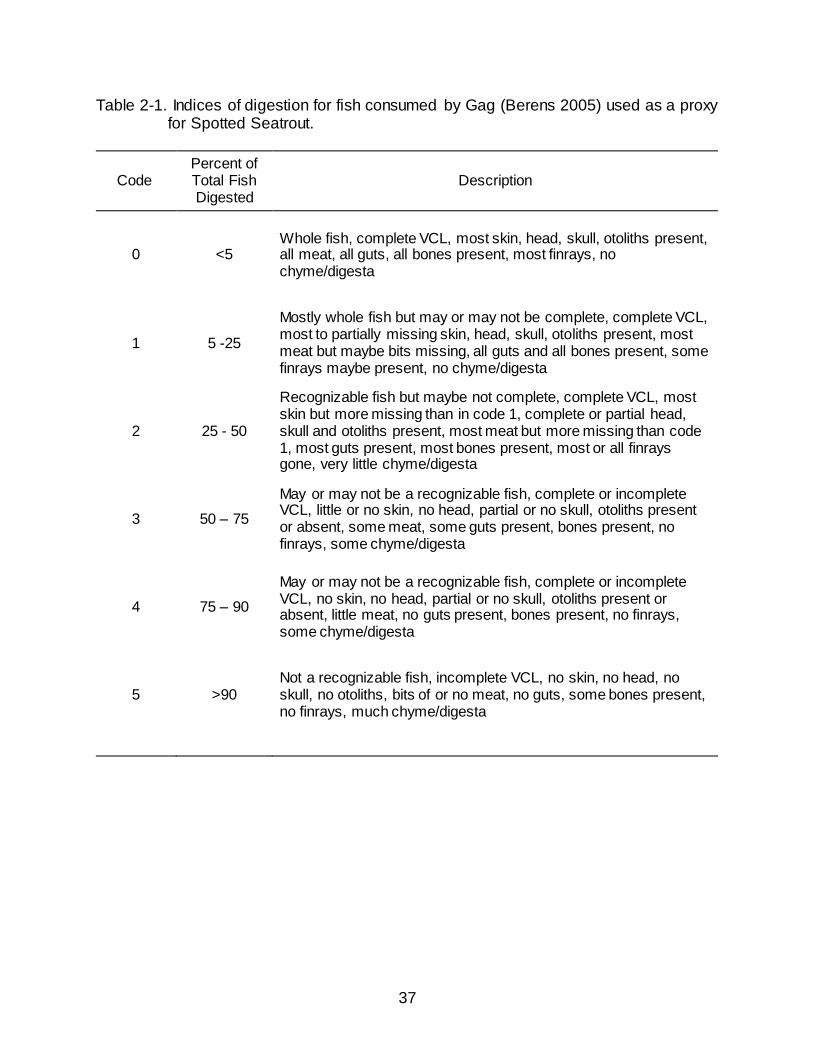
Table 2-1. Indices of digestion for fish consumed by Gag (Berens 2005) used as a proxy for Spotted Seatrout.
Code Percent of Total Fish Digested
Description
0 <5 Whole fish, complete VCL, most skin, head, skull, otoliths present, all meat, all guts, all bones present, most finrays, no chyme/digesta
1 5 -25
Mostly whole fish but may or may not be complete, complete VCL, most to partially missing skin, head, skull, otoliths present, most meat but maybe bits missing, all guts and all bones present, some finrays maybe present, no chyme/digesta
2 25 - 50
Recognizable fish but maybe not complete, complete VCL, most skin but more missing than in code 1, complete or partial head, skull and otoliths present, most meat but more missing than code 1, most guts present, most bones present, most or all finrays gone, very little chyme/digesta
3 50 – 75
May or may not be a recognizable fish, complete or incomplete VCL, little or no skin, no head, partial or no skull, otoliths present or absent, some meat, some guts present, bones present, no finrays, some chyme/digesta
4 75 – 90
May or may not be a recognizable fish, complete or incomplete VCL, no skin, no head, partial or no skull, otoliths present or absent, little meat, no guts present, bones present, no finrays, some chyme/digesta
5 >90 Not a recognizable fish, incomplete VCL, no skin, no head, no skull, no otoliths, bits of or no meat, no guts, some bones present, no finrays, much chyme/digesta
38
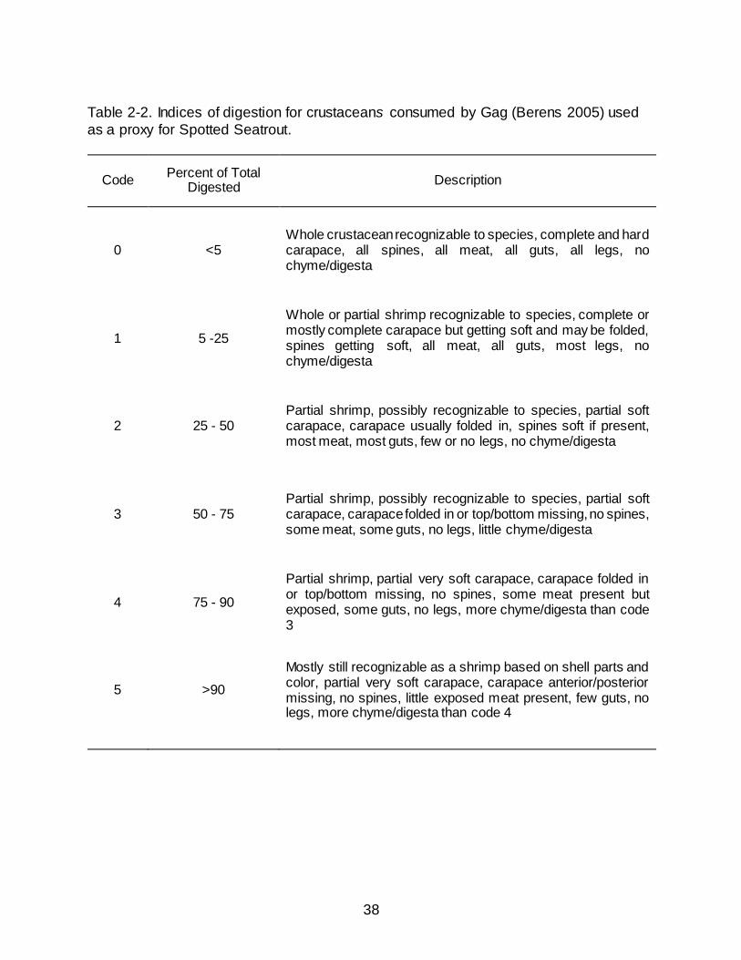
Table 2-2. Indices of digestion for crustaceans consumed by Gag (Berens 2005) used
as a proxy for Spotted Seatrout.
Code Percent of Total
Digested Description
0 <5 Whole crustacean recognizable to species, complete and hard carapace, all spines, all meat, all guts, all legs, no chyme/digesta
1 5 -25
Whole or partial shrimp recognizable to species, complete or mostly complete carapace but getting soft and may be folded, spines getting soft, all meat, all guts, most legs, no chyme/digesta
2 25 - 50 Partial shrimp, possibly recognizable to species, partial soft carapace, carapace usually folded in, spines soft if present, most meat, most guts, few or no legs, no chyme/digesta
3 50 - 75 Partial shrimp, possibly recognizable to species, partial soft carapace, carapace folded in or top/bottom missing, no spines, some meat, some guts, no legs, little chyme/digesta
4 75 - 90
Partial shrimp, partial very soft carapace, carapace folded in or top/bottom missing, no spines, some meat present but exposed, some guts, no legs, more chyme/digesta than code 3
5 >90
Mostly still recognizable as a shrimp based on shell parts and color, partial very soft carapace, carapace anterior/posterior missing, no spines, little exposed meat present, few guts, no legs, more chyme/digesta than code 4
39
CHAPTER 3 RESULTS
Spotted Seatrout Sampling
Spotted Seatrout were collected between June 2013 and June 2016. In total, 903
Spotted Seatrout were collected from Florida and Louisiana. Sampling in Florida yielded
467 Spotted Seatrout of which 227 contained stomach contents; fish ranged in size from
153-585 mm MTL (Figure 3-1). Louisiana sampling produced 436 Spotted Seatrout of
which 245 contained stomach contents; fish ranged in size from 213-455 mm MTL
(Figure 3-1). The percentage of empty stomachs was lowest in fish collected from
Venice, LA (32.89%) and was highest in the West Florida region (55.85%) (Table 3-1).
Feeding Chronology
Overall, the total percentage of empty stomachs from Spotted Seatrout was
47.72% (Table 3-1). A significant difference in the frequency distribution of empty and
non-empty stomachs was detected for collections between 0600-2000 h (2 = 46.3, P <
0.0001) and a bimodal distribution was present (Figure 3-2). Strong increases in the
percentage of stomachs containing prey were apparent in the mid-morning, between
0800-1000 h, and late afternoon, between 1600-1800 h, and indicated relative
increases in feeding activity. Low percentages representing the greatest occurrence of
empty stomachs occurred in the early morning between 0600-0800 h, mid-afternoon
between 1400-1600 h, and evening between 1800-2000 h (Figure 3-2).
Difference in the mean wet weight of stomach contents (as a percentage of body
weight) by collection time period was not statistically significant (ANOVA; P = 0.218)
(Figure 3-3). There appeared to be an overall trend of an increase in stomach content
40
weight in the mid to late morning (0800-1200 h) followed by lower and more variable
stomach content weights.
There was a significant difference in the frequency of digestion codes as a
function of collection time (2 = 99.1, P < 0.0001) and a distinct bimodal distribution in
codes (0-2) (<50% digested) indicates more recent feeding (Figure 3-4). The greatest
frequency of the least digested prey items (indicating recent feeding) occurred in the
early morning (0600-0800 h) and midafternoon (1400-1600 h), while the greatest
frequency of the most digested prey items occurred at mid-day (1200-1400 h) and late
evening (1800-2000 h).
Collectively, the percentage of empty stomachs, average weight of stomach
contents, and frequency of digestion code occurrence indicated that Spotted Seatrout
were primarily feeding during the mid-morning (0800-1000 h) and may exhibit a second
feeding period in the afternoon.
Post-Spill Contemporary Diet by Location
Stomach Content Analysis by Location
Of the 903 fish collected, stomachs from 434 fish were empty while 472
stomachs contained prey items. A total of 1,451 prey items were identified. A digestion
code of 5 (>90% digested) was assigned to 641 prey items; however, only 40 refractory
stomachs (stomachs only containing prey with a digestion code of 5), which contained a
total of 61 prey items, were identified. Removal of these refractory stomachs and prey
items made little impact on results (changing values by <2%) and were therefore
included in all analyses. All prey accumulation curves increased by 5% or less over the
last 10 stomachs analyzed indicating that the diet was well described (Figure 3-5).
41
Regressions and values used to back calculate and estimate whole weights of prey
items are presented in Table 3-2.
Diet Composition in Florida
Teleost fishes made up the greatest percentage of the diet in Spotted Seatrout
collected in Florida by all metrics (74.9% O, 61.0% N, 76.1% RW) (Table 3-3).
Demersal fishes contributed to 42.7% O, 27.7% N, and 58.9% RW of the total diet with
Pinfish Lagodon rhomboides being the greatest contributor of occurrence and RW
(22.9% O, 13.3%N, 32.5% RW), while Anchoa sp. was the most numerically abundant
species but contributed little in weight (20.3% O, 18.4% N, 3.6% RW). Crustaceans
occurred in over half of the stomachs containing prey (58.6% O) while contributing to
over a third of the numerical abundance (38.0% N) as well as 23.9% RW. Decapod
shrimp were the majority of crustaceans by all metrics represented in the diet of Spotted
Seatrout in Florida (54.6% O, 33.9% N, 23.1% RW). Penaeid shrimp accounted for
13.7% RW and appeared in 18.1% of non-empty stomachs. Unidentifiable shrimp
occurred in 30.0% of non-empty stomachs.
Dietary contributions between Big Bend, FL, and West Florida were similar
(Table 3-4). Teleost fishes occurred in over 70% of non-empty stomachs and accounted
for approximately 75% of the total RW in each location. In West Florida, the occurrence
and numerical abundance of demersal fish was roughly 20% greater than in the Big
Bend, however, the contribution to weight was similar (Table 3-4). Lagodon rhomboides
dominated the presence of demersal fish in West Florida (38.9% O, 23.7% N, 50.7%
RW) and was present in the diet of Big Bend fish (7.0% O, 3.8% N, 17.2% RW) but at
reduced percentages. Pelagic fishes occurred in over three times as many stomachs
42
from Big Bend than from West Florida (37.7% versus 9.7 % O, respectively). Clupeiform
fishes, specifically from the families Engraulidae and Clupeidae, contributed to 36.8%
O, 37.9% N, 11.9% RW of the pelagic fish in Big Bend and only 8.0% O, 5.0% N, 1.2%
RW in West Florida. Crustaceans, even at various groups (i.e. decapod crab, decapod
shrimp, unidentified shrimp), also had similar percentages between locations.
Diet Composition in Louisiana
As in Florida, the diet of Spotted Seatrout collected in Louisiana was dominated
by teleosts (79.2% O, 69.1% N, 84.5% RW) (Table 3-3). Demersal and pelagic fishes
occurred in nearly the same percentage of stomachs containing prey (40.0% and 40.8%
O, respectively). Numerical abundance of pelagic fishes (47.3% N) was over twice that
of demersal fishes (19.0% N), although the percentages of RW between demersal
fishes (43.1% RW) and pelagic fishes (35.4% RW) were similar. Poecilids, specifically
Sailfin molly Poecilia latipinna (11.4% O, 7.0% N, 8.0% RW) and Sciaenids, specifically
Micropogonias undulates (11.0% O, 4.1% N, 11.5% RW) were noticeable contributors
to the demersal fish category. Engraulids (30.6% O, 43.1% N, 13.7% RW) and clupeids
(13.5% O, 3.6% N, 20.5% RW) were also key contributors to the pelagic fish category.
Crustaceans were observed in over half of the stomachs containing prey (57.1% O) and
contributed 30.9% N yet provided less than a quarter of the RW (15.5%). The bulk of
the crustaceans came from decapod shrimp (31.8% O, 12.4% N, 13.1% RW), which
consisted mainly of penaeids and unidentified shrimp. Decapod Crabs had an increased
presence in fish collected in Louisiana (19.6% O, 8.7% N, 2.3% RW) compared to
Florida (4.8% O, 2.2% N, 0.8% RW).
43
Spotted Seatrout collected in Venice had a greater contribution of teleost fishes
to their diet (92.0% O, 72.2% N, 92.6% RW) than in Grand Isle (70.3% O, 63.1% N,
79.3% RW) (Table 3-5), this can be attributed to the large proportion of pelagic fish
(specifically clupeiforms) present in the Venice diet. Spotted Seatrout consumed more
demersal fish in Grand Isle (53.8% O, 49.2% N, 56.7% RW) than in Venice (20.0% O,
3.8% N, 21.6% RW). Driving the differences in demersal fishes was the consumption of
Cyprinodontiformes, primarily P. latipinna, and Sciaenids, primarily M. undulatus, which
were found only in the diets of Spotted Seatrout collected in Grand Isle and not in
Venice. Differences in the consumption of crustaceans were also apparent numerically
and by RW between the diets of Spotted Seatrout collected in Grand Isle (52.4% O,
36.9% N, 20.7% RW) and Venice (64.0% O, 27.8% N, 7.4% RW). This difference was
due to high percentages of Decapod shrimp in the diet of Grand Isle Spotted Seatrout
and low percentages of decapod shrimp in the diet of Venice Spotted Seatrout.
Additionally, Venice Spotted Seatrout had high occurrences of amphipods and decapod
crabs. Amphipods were largely absent and decapod crabs occurred in fewer of the non-
empty Spotted Seatrout stomachs collected in Grand Isle.
Indices of Relative Importance by Location
Relative importance of prey items was based on two levels of progressively finer
detail for comparing the overlying prey categories. Based on RW, the Index of Relative
Importance (IRI) for Florida and Louisiana by coarse groupings of Crustacea, Teleost,
Mollusca, and Unidentified taxa indicated that teleost fishes were the most important
prey category followed by crustaceans (Table 3-3). While present in the diet, molluscs
and unidentified taxa were encountered rarely and their IRI’s were therefore 0. The IRI
44
for teleost fishes was lowest in West Florida (72.2% IRI) (Table 3-4) and greatest in
Venice (87.4% IRI) (Table 3-5). Consequently, the IRI of Crustaceans was greatest in
West Florida (27.8% IRI) and least in Venice (12.6% IRI).
Finer scaled IRI was calculated for the following groups: Amphipod, Decapod
crab, Isopod, Decapod shrimp, Demersal fish, Pelagic fish, Unknown fish, Gastropod,
and Unidentified taxa. This higher resolution IRI followed a similar pattern with fishes
being the main contributors in each state (Table 3-3). However, demersal fishes (47.1%
IRI) and pelagic fishes (48.0% IRI) were prioritized in Florida and Louisiana,
respectively. In Florida, the most important prey items, in order, were demersal fishes,
decapod shrimp, and pelagic fishes (Table 3-4). In Louisiana, the most important prey
items, in order, were pelagic fishes, demersal fishes, and decapod shrimp (Table 3-5).
In Florida, decapod shrimp held similar importance in both Big Bend and West Florida
(38.4% and 36.8% IRI, respectively) (Table 3-4). Demersal fishes were more important
in West Florida (57.0% IRI) than in Big Bend (32.9%). Pelagic fishes were 25.6% IRI
and 0.8% IRI in Big Bend and West Florida, respectively. In Louisiana, demersal fishes
were 68.3% IRI in Grand Isle and 4.2% IRI in Venice, whereas, pelagic fishes were
5.3% and 87.0% in Grand Isle and Venice, respectively (Table 3-5). Decapod shrimp
were more important in Grand Isle (24.3% IRI) than in Venice (1.3% IRI). Notable was
the increased importance of Amphipod (4.0% IRI) and Decapod crab (2.9% IRI) in
Venice, relative to other locations.
Dietary Overlap and Breadth in Spotted Seatrout by Location
Between Florida and Louisiana, Schoener’s Index of overlap based on RW was
0.45. Schoener’s Index ranged from 0.14-0.62 between individual locations (Table 3-6).
45
Overlap was highest, and subsequently biologically significant, among fish collected in
Grand Isle, LA, and Big Bend, FL (α = 0.62). In contrast, overlap between Venice, LA,
and West Florida was the lowest (α = 0.14). Dietary overlap was marginal among
Spotted Seatrout collected in Grand Isle and Venice (α = 0.43) and in Big Bend and
West Florida (α = 0.50).
Dietary overlap using the Simplified Morisita Index based on RW exhibited a
similar pattern as those derived from the Schoener’s Index. Between Florida and
Louisiana, dietary overlap using the Simplified Morisita Index was 0.49. The Simplified
Morisita Index ranged from 0.07-0.81 for individual locations (Table 3-6). Overlap was
highest, and biologically significant, between fish collected in Grand Isle, LA and Big
Bend, FL (CH = 0.81). Overlap between Venice, LA, and West Florida was the lowest
(CH = 0.07). Overlap of the diet was marginal between Grand Isle and Venice, Venice
and Big Bend, and Big Bend and West Florida.
Dietary breadth was relatively similar between Florida (J’ = 0.62) and Louisiana
(J’ = 0.69) when calculated with the RW of prey items (Table 3-7). Breadth of the diet
was similar across individual locations and ranged from 0.53-0.69. The broadest diet
was identified in the Big Bend (J’= 0.69) and the narrowest diet was observed in West
Florida (J’= 0.53).
Similarity in the Diet of Spotted Seatrout by Location
Despite global R values being very close to zero (R = 0.131, P = 0.001),
indicating high similarity between sites, ANOSIM detected statistical differences in the
diet of Spotted Seatrout based on location (Table 3-8). Low R values coupled with
statistical significance suggests that diets are not identical but exhibit high amounts of
46
overlap. The diets of Grand Isle and West Florida (R = 0.109), Grand Isle and Big Bend
(R = 0.069), West Florida and Big Bend (R = 0.077), and Big Bend and Venice (R =
0.099) were the most similar. The diet between Grand Isle and Venice showed
moderate dissimilarity (R = 0.179). The greatest dissimilarity, while still low in relation to
the possible maximum value of R (i.e. 1), was observed between the diet of West
Florida and Venice (R = 0.295).
SIMPER analysis identified prey items contributing to dissimilarities of pairwise
comparisons in which the pairwise R was greater than the global R indicating the
greatest dissimilarities in diet. SIMPER analysis for the diets of Spotted Seatrout
collected in Grand Isle and Venice indicated that Anchoa sp. occurred in a greater
dietary abundance by RW in Venice than in Grand Isle and contributed the greatest
percentage to the observed dissimilarity (Table 3-9); shrimp were the second greatest
contributor. Similarly, Anchoa sp. drove the dissimilarity between West Florida and
Venice (Table 3-9). West Florida also had a high abundance of Pinfish, which were not
observed in the Venice diet. Shrimp also occurred in higher abundances in West Florida
than in Venice.
Four outliers were removed from the initial MDS, each of these stomachs
contained only a single rare prey item (each occurring in ≤ 2 stomachs). The resulting
MDS plot of the original core cluster (Figure 3-6) had low stress (0.07) indicating a high
goodness of fit and portrayed a tight cluster of stomachs, which supported the similarity
in the diet of Spotted Seatrout identified in the ANOSIM. In other words, the MDS plot
displayed no distinctly segregated groupings based on location. However, as indicated
with the low but significant R values, the diets from each location were not exactly the
47
same but experienced high overlap indicated by the tight, and overlapping, grouping of
each location. For instance, the high similarity between Grand Isle and Big Bend
identified in the ANOSIM (R = 0.069) is reflected in the large amount of overlap between
those points on the MDS. Further, the similarity in the ANOSIM was lowest between
West Florida and Venice (R = 0.295), which was supported by little overlap of points in
the MDS, yet overall the points are still in close proximity.
Post-Spill Contemporary Diet of Spotted Seatrout by Season
Stomach Content Analysis by Season
Dietary analysis by location deemed the diet similar enough to pool all locations
for a seasonal assessment of the Spotted Seatrout diet. The greatest number of
Spotted Seatrout were collected during the fall and the fewest were collected during
winter (Table 3-10). Seasonal comparisons of the Spotted Seatrout diet were made
between spring, summer, and fall; winter was excluded due to low sample size.
Seasonal Composition of the Diet
Spotted Seatrout collected during the spring had the greatest overall percentages
of crustaceans (80.2% O, 57.3% N, 43.9% RW) present in the diet (Table 3-11).
Decapod crabs (18.0% O, 7.9% N, 4.7% RW) and decapod shrimp (67.6% O, 45.9% N,
41.0% RW) contributed more during the spring than in any other season. The
occurrence (64.9% O) and numerical abundance (42.7% N) of teleosts was less than
crustaceans during the spring but teleost contributions by weight (56.1% RW) was
similar to crustaceans. In the spring, teleost totals were mainly composed of benthic fish
(53.2% O, 34.1% N, 35.6% RW), specifically Micropogonias undulatus (15.3% O, 10.4%
48
N, 14.9% RW) and Lagodon rhomboides (18.9% O, 8.6% N, 12.1% RW). Noticeably
less than in other seasons was the contribution of pelagic fishes (4.5% O, 1.8% N, 2.0%
RW) to the diet of Spotted Seatrout in the spring.
Compared to the spring, summer months saw a decline in crustaceans (49.2%
O, 32.9% N, 23.6% RW) and an increase in teleosts (69.8% O, 66.7% N, 76.4% RW)
(Table 3-11). The greatest difference between spring and summer was the increase of
pelagic fish (29.4% O, 30.6% N, 24.2% RW), particularly those in the family Clupeidae.
Percentages of benthic fish (38.9% O, 26.1% N, 45.6% RW) remained relatively similar
compared to spring.
The contribution of crustaceans continued to decline into the fall (52.4% O,
26.5% N, 11.2% RW) while contributions of teleosts peaked (86.7% O, 73.2% N, 88.8%
RW). Compared to summer, the occurrence and numerical abundance of decapod
crabs increased but contributed little percentages of weight. Amphipods in the family
Gammaridea increased in both occurrence and numerical abundance during fall months
but contributed very little to percentages of weight due to their small size. Decapod
shrimp, while still occurring in 30.9% of stomachs, contributed 10.2% RW, which was
less than half of their contribution to weight during spring and summer. The occurrence
(36.5% O) and numerical abundance (17.3% N) of benthic fish dipped in the fall when
compared to spring and summer but still contributed over half of the weight (58.1% RW)
to the overall fall diet. Most noticeable was the peak in pelagic fish; pelagic fish, mainly
Engraulids and Clupeids, contributed more during the fall than in any other season
(48.1% O, 51.7% N, 25.7% RW).
49
Indices of Relative Importance by Season
The IRI for spring, based on coarse groupings, indicated that crustaceans were
the most important prey item (Table 3-11). The IRI of spring, when calculated based on
finer groups, indicated that decapod shrimp (57.7% IRI) were the most important prey
item followed by demersal fish (36.2% IRI). During the summer months, relative prey
importance of coarse groupings shifted towards teleosts (78.5% IRI) and the importance
of crustaceans declined (21.5% IRI). Finer groupings revealed that demersal fish
(40.8% IRI) were the most important followed by decapod shrimp (33.1% IRI) and
pelagic fish (23.6% IRI). The IRI for fall was dominated by teleosts (87.7% RW IRI) and
the importance of crustaceans dropped considerably (12.3% RW IRI). Finer groupings
identified pelagic fish (49.9% IRI) as the most important prey group in the fall followed
by demersal fish (36.6% IRI). Importance of decapod shrimp (8.4% IRI) was much lower
in the fall than in spring or summer.
Measures of Dietary Overlap and Breadth by Season
Schoener’s Index of Overlap based on RW ranged from 0.51-0.67. Fish collected
during the summer compared to the fall had the highest overlap (α = 0.67), followed
closely by those collected in the spring and summer (α = 0.64), each of which were
considered biologically significant overlap. The diet of fish collected in the spring
compared to fall had moderate overlap (α = 0.51).
The Simplified Morisita Index of Overlap based on RW ranged from 0.65-0.88 of
which all were biologically significant. Fish collected during the summer and fall had the
highest overlap (CH = 0.88), followed closely by those collected in the spring and
50
summer (CH = 0.78). The diet of fish collected in the spring compared to fall had
significant overlap (CH = 0.65).
By season, dietary breadth was broad during all seasons, indicating a
generalized diet for Spotted Seatrout in the spring, summer and fall (Table 3-7).
Similarity in the Diet by Season
ANOSIM detected statistical differences in the seasonal diet of Spotted Seatrout
despite the global R value being very close to zero (R = 0.073, P = 0.0001) (Table 3-8).
Similarity in the diet was greatest between spring and summer (R = 0.021) and summer
and fall (R = 0.068). Diet similarity was statistically different between spring and fall (R =
0.104), however this dissimilarity is likely inconsequentially small in regards to the
possible range of R (i.e. 0-1). SIMPER indicated that seasonal dissimilarities between
spring and fall were attributed to high dietary abundance by RW of Anchoa sp. during
the fall which were scarcely observed in the spring diet (Table 3-12). Additionally,
shrimp occurred at much higher dietary abundances by RW during the spring than in
the fall. The MDS plot supported the similarity among seasons as the individual clusters
were largely overlapping but were not tightly grouped, indicating increased variation
(Figure 3-7). As indicated with ANOSIM, spring and fall were least similar and overlap
appeared to be less in the MDS plot compared to overlap of the other seasonal clusters.
However, data for spring and fall were still close in proximity and no complete
segregation was apparent, supporting the inconsequentially small dissimilarity indicated
by the R value.
51
Size-Dependent Diet of Spotted Seatrout
As with the seasonal assessment of diet, Spotted Seatrout across all locations
were combined to assess the diet based on fish size. Sample sizes of the Spotted
Seatrout size bins were as follows: 150-299 mm TL (size 1, n = 172), 300-350 mm TL
(size 2, n = 167), 350-600 mm TL (size 3, n = 133).
Diet Composition by Size
Overall, crustaceans contributed nearly equal parts by occurrence and numerical
abundance across all size bins (Table 3-13), but contributed less by %RW to the diet of
the largest Spotted Seatrout (16.1%) than the smallest Spotted Seatrout (24.0%).
Noticeable among the decapod shrimp contribution between size groups was the
diversity in contribution by many families in the diet of size 1 and 2 Spotted Seatrout,
opposed to mainly just penaeid shrimp amongst size 3 Spotted Seatrout. Conversely,
teleosts contributed more by %RW to the diet of larger Spotted Seatrout (83.9%) than
smaller Spotted Seatrout (76.0%). Among teleost prey categories, sciaenids and Pinfish
occurred most frequently, were most numerically abundant, and contributed the most by
%RW to the diet of Spotted Seatrout in size 3 than in any other size group. Whereas the
converse was true regarding the engraulid Anchoa sp. among the size 1 Spotted
Seatrout compared to the size 3 Spotted Seatrout.
Indices of Relative Importance by Size
The importance of crustaceans was relatively similar across size groups and
ranged from 23% IRI to 21% IRI from the smallest to largest Spotted Seatrout,
respectively (Table 3-13). Similarly, the IRI of teleosts was relatively consistent across
52
size groups and ranged from 77% (size 1) to 79% (size 3). Molluscs and unidentified
taxa were rarely encountered and therefore, their IRI values were 0.
Finer IRI categories revealed a consistent decapod shrimp IRI, ranging from 23%
to 25% across all size groups (Table 3-13). The IRI of demersal fishes increased
markedly with Spotted Seatrout size, increasing from 16.8% in size group 1 to 67.9% in
size group 3. Pelagic fishes, particularly Anchoa sp., decreased in importance as fish
size increased, and was 52.6% IRI in size group 1 and only 5.3% IRI in size group 3.
Measures of Dietary Overlap and Breadth by Size
Schoener’s Index of Overlap based on RW ranged from 0.56-0.82. Fish in size
groups 1 and 2 had the highest overlap (α = 0.82), followed by those in size groups 2
and 3 (α = 0.61), each of which were considered biologically significant overlap. The
diet of fish in size groups 1 and 3 had moderate overlap (α = 0.56).
The Simplified Morisita Index of Overlap based on RW ranged from 0.63-0.94 of
which all were biologically significant. Fish in size groups 1 and 2 had the highest
overlap (CH = 0.88), followed by those in size groups 2 and 3 (CH = 0.74). The diet of
fish in size groups 1 and 3 had the lowest but still biologically significant overlap (CH =
0.65).
Dietary breadth was broad across all size groups, indicating a generalized diet
for Spotted Seatrout regardless of size (size 1: H’ = 2.17, J’ = 0.71; size 2: H’ = 2.29, J’
= 0.72; size 3: H’ = 2.05, J’ = 0.64).
53
Similarity in the Diet by Size
ANOSIM detected statistical differences in the size-dependent diet of Spotted
Seatrout despite the global R value being very close to zero (R = 0.04, P = 0.0001).
Only the diets of the smallest (1: 150 - 299 mm TL) and largest (3: > 350 mm TL) size
bins were statistically different (R = 0.085). SIMPER identified a greater abundance of
generally larger fish in the diet of Spotted Seatrout in size group 3 (i.e., sciaenids,
Pinfish, clupeids) and a much higher abundance of Anchoa spp. in group 1 (Table 3-
14). The MDS plot showed overlapping clusters of each size group, which supports the
low R values observed in the ANOSIM, while the clusters of size groups 1 and 3
showed the increased variation and the least relative overlap (Figure 3-8).
Pre-and Post-Spill Comparison of Spotted Seatrout Diet
Overall, estimation of %O and %DW from the present study, Simonsen’s study
(2008; Table 3-15), and Russell (2005) indicated that the diversity of fish prey types
consumed post-spill was greater than pre-spill (Table 3-16). When prey categories were
re-grouped to lower potential bias associated with differences in the resolution of prey
identifications (Table 3-17), the present study had a greater occurrence of both teleosts
and crustaceans than either pre-spill study. However, when considered by %DW,
results were most similar between the present study and Russell (2005) (Table 3-17),
with the %DW of teleosts and crustaceans differing by <10% and <6%, respectively.
Comparatively, the present study observed approximately 23% more teleosts and 23%
less crustaceans by DW than Simonsen (2008). Similarly, Russell (2005) also observed
more teleosts and less crustaceans than Simonsen (2008).
54
At a finer level of prey category comparison, Unidentified/other fish, penaeid
shrimp, B. patronus, and M. undulatus, contributed most to the diet of Spotted Seatrout
both pre- and post-spill. Molluscs and polychaetes were observed in the pre-spill diet in
small amounts but were absent in the post-spill diet. Simonsen (2008) observed
unidentified/other fish, the engraulid Anchoa spp., and penaeid shrimp as the most
frequently occurring prey items in the pre-spill diet of Spotted Seatrout in Grand Isle, LA
(Table 3-17). However, when considered by DW, Simonsen found that penaeid shrimp
was the single greatest contributor, followed by Anchoa sp., unidentified/other fish, and
the clupeid B. patronus. In the pre-spill diet of Spotted Seatrout observed by Russell
(2005), unidentified/other fish, penaeid shrimp, and Anchoa sp. were the most
frequently occurring prey items. When considered by DW, Russell found
unidentified/other fish, penaeid shrimp, and clupeids, were the main contributors to the
pre-spill Spotted Seatrout diet (Table 3-17). Comparatively, once prey identified in the
present study were redistributed to match pre-spill prey categories, the observed
occurrence of unidentified/other fish was 27% greater than observed by Simonsen
(2008), and approximately 5% less than observed by Russell (2005). Penaeid shrimp
occurred more frequently in the present study than in Simonsen’s study, however, they
contributed more to the DW (24%) in the latter study.
Overlap between the pre- and post-spill diets of Spotted Seatrout ranged from
0.56 to 0.92 (Table 3-18). Overlap was high and biologically significant among pre- and
post-spill studies when considered by overall prey categories (teleosts, crustaceans,
molluscs, polychaete). When considered by prey categories at finer resolution, overlap
was high and biologically significant between the present study and Russell (2005) and
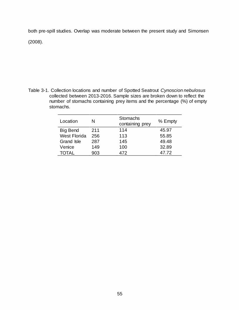
55
both pre-spill studies. Overlap was moderate between the present study and Simonsen
(2008).
Table 3-1. Collection locations and number of Spotted Seatrout Cynoscion nebulosus
collected between 2013-2016. Sample sizes are broken down to reflect the number of stomachs containing prey items and the percentage (%) of empty
stomachs.
Location N Stomachs
containing prey % Empty
Big Bend 211 114 45.97
West Florida 256 113 55.85
Grand Isle 287 145 49.48
Venice 149 100 32.89
TOTAL 903 472 47.72
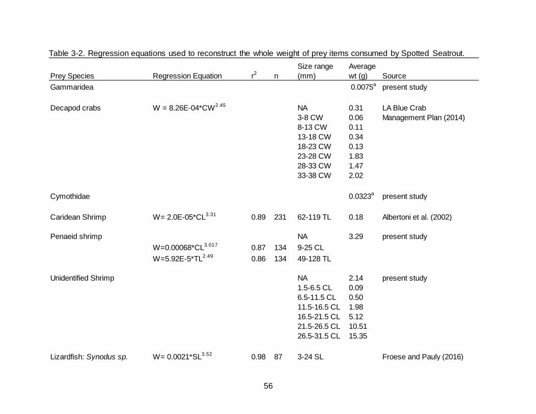
56
Table 3-2. Regression equations used to reconstruct the whole weight of prey items consumed by Spotted Seatrout.
Prey Species Regression Equation r2 n
Size range
(mm)
Average
wt (g) Source
Gammaridea 0.0075a present study
Decapod crabs W = 8.26E-04*CW2.45 NA 0.31 LA Blue Crab
3-8 CW 0.06 Management Plan (2014)
8-13 CW 0.11
13-18 CW 0.34
18-23 CW 0.13
23-28 CW 1.83
28-33 CW 1.47
33-38 CW 2.02
Cymothidae 0.0323a present study
Caridean Shrimp W= 2.0E-05*CL3.31 0.89 231 62-119 TL 0.18 Albertoni et al. (2002)
Penaeid shrimp NA 3.29 present study
W=0.00068*CL3.017 0.87 134 9-25 CL
W=5.92E-5*TL2.49 0.86 134 49-128 TL
Unidentified Shrimp NA 2.14 present study
1.5-6.5 CL 0.09
6.5-11.5 CL 0.50
11.5-16.5 CL 1.98
16.5-21.5 CL 5.12
21.5-26.5 CL 10.51
26.5-31.5 CL 15.35
Lizardfish: Synodus sp. W= 0.0021*SL3.52 0.98 87 3-24 SL Froese and Pauly (2016)
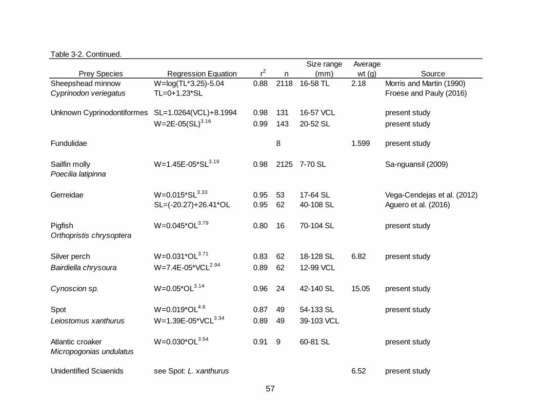
57
Prey Species Regression Equation r2 n
Size range
(mm)
Average
wt (g) Source
Sheepshead minnow W=log(TL*3.25)-5.04 0.88 2118 16-58 TL 2.18 Morris and Martin (1990)
Cyprinodon veriegatus TL=0+1.23*SL Froese and Pauly (2016)
Unknown Cyprinodontiformes SL=1.0264(VCL)+8.1994 0.98 131 16-57 VCL present study
W=2E-05(SL)3.16 0.99 143 20-52 SL present study
Fundulidae 8 1.599 present study
Sailfin molly W=1.45E-05*SL3.19 0.98 2125 7-70 SL Sa-nguansil (2009)
Poecilia latipinna
Gerreidae W=0.015*SL3.33 0.95 53 17-64 SL Vega-Cendejas et al. (2012)
SL=(-20.27)+26.41*OL 0.95 62 40-108 SL Aguero et al. (2016)
Pigfish W=0.045*OL3.79 0.80 16 70-104 SL present study
Orthopristis chrysoptera
Silver perch W=0.031*OL3.71 0.83 62 18-128 SL 6.82 present study
Bairdiella chrysoura W=7.4E-05*VCL2.94 0.89 62 12-99 VCL
Cynoscion sp. W=0.05*OL3.14 0.96 24 42-140 SL 15.05 present study
Spot W=0.019*OL4.6 0.87 49 54-133 SL present study
Leiostomus xanthurus W=1.39E-05*VCL3.34 0.89 49 39-103 VCL
Atlantic croaker W=0.030*OL3.54 0.91 9 60-81 SL present study
Micropogonias undulatus
Unidentified Sciaenids see Spot: L. xanthurus 6.52 present study
Table 3-2. Continued.
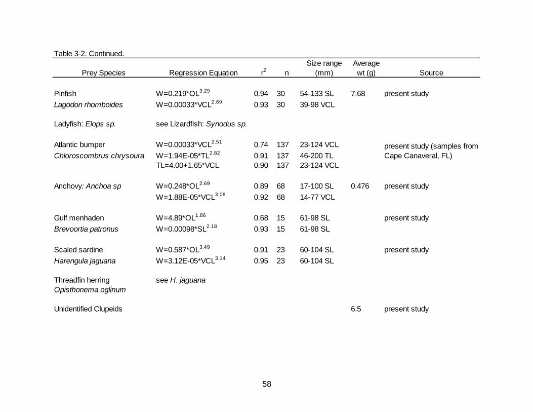
58
Prey Species Regression Equation r2 n
Size range
(mm)
Average
wt (g) Source
Pinfish W=0.219*OL3.29 0.94 30 54-133 SL 7.68 present study
Lagodon rhomboides W=0.00033*VCL2.69 0.93 30 39-98 VCL
Ladyfish: Elops sp. see Lizardfish: Synodus sp.
Atlantic bumper W=0.00033*VCL2.51 0.74 137 23-124 VCL
Chloroscombrus chrysoura W=1.94E-05*TL2.82 0.91 137 46-200 TL
TL=4.00+1.65*VCL 0.90 137 23-124 VCL
Anchovy: Anchoa sp W=0.248*OL2.69 0.89 68 17-100 SL 0.476 present study
W=1.88E-05*VCL3.08 0.92 68 14-77 VCL
Gulf menhaden W=4.89*OL1.86 0.68 15 61-98 SL present study
Brevoortia patronus W=0.00098*SL2.18 0.93 15 61-98 SL
Scaled sardine W=0.587*OL3.49 0.91 23 60-104 SL present study
Harengula jaguana W=3.12E-05*VCL3.14 0.95 23 60-104 SL
Threadfin herring see H. jaguana
Opisthonema oglinum
Unidentified Clupeids 6.5 present study
Table 3-2. Continued.
present study (samples from
Cape Canaveral, FL)
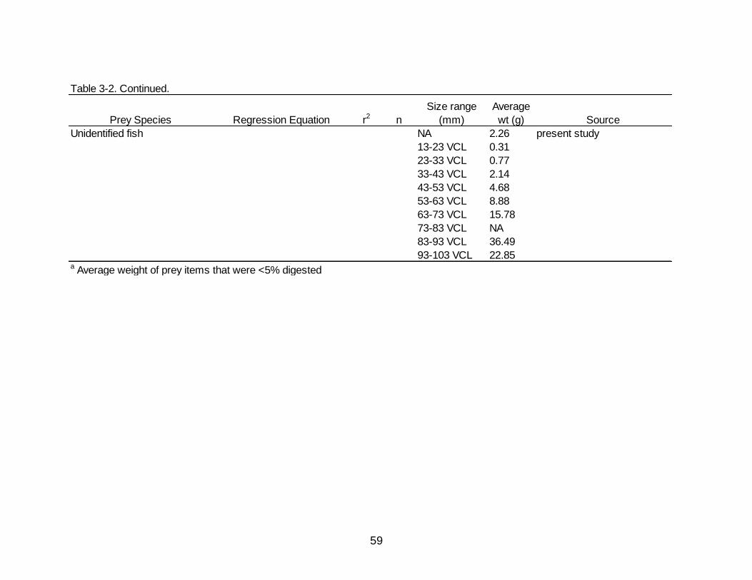
59
Prey Species Regression Equation r2 n
Size range
(mm)
Average
wt (g) Source
Unidentified fish NA 2.26 present study
13-23 VCL 0.31
23-33 VCL 0.77
33-43 VCL 2.14
43-53 VCL 4.68
53-63 VCL 8.88
63-73 VCL 15.78
73-83 VCL NA
83-93 VCL 36.49
93-103 VCL 22.85a Average weight of prey items that were <5% digested
Table 3-2. Continued.
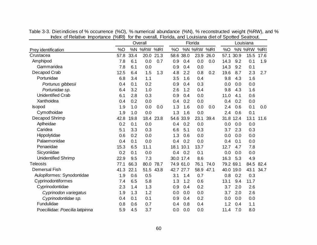
60
Table 3-3. Diet indicies of % occurrence (%O), % numerical abundance (%N), % reconstructed weight (%RW), and % Index of Relative Importance (%IRI) for the overall, Florida, and Louisiana diet of Spotted Seatrout.
%O %N %RW %IRI %O %N %RW %IRI %O %N %RW %IRI
57.8 33.4 20.0 21.3 58.6 38.0 23.9 26.0 57.1 30.9 15.5 17.6
7.8 6.1 0.0 0.7 0.9 0.4 0.0 0.0 14.3 9.2 0.1 1.9
7.8 6.1 0.0 0.9 0.4 0.0 14.3 9.2 0.1
12.5 6.4 1.5 1.3 4.8 2.2 0.8 0.2 19.6 8.7 2.3 2.7
6.8 3.4 1.1 3.5 1.6 0.4 9.8 4.3 1.6
Portunus gibbesii 0.4 0.1 0.2 0.9 0.4 0.3 0.0 0.0 0.0
Portunidae sp. 6.4 3.2 1.0 2.6 1.2 0.4 9.8 4.3 1.6
6.1 2.8 0.3 0.9 0.4 0.0 11.0 4.1 0.6
0.4 0.2 0.0 0.4 0.2 0.0 0.4 0.2 0.0
1.9 1.0 0.0 0.0 1.3 1.6 0.0 0.0 2.4 0.6 0.1 0.0
1.9 1.0 0.0 1.3 1.6 0.0 2.4 0.6 0.1
42.8 19.8 18.4 23.8 54.6 33.9 23.1 39.4 31.8 12.4 13.1 11.6
0.2 0.1 0.0 0.4 0.2 0.0 0.0 0.0 0.0
5.1 3.3 0.3 6.6 5.1 0.3 3.7 2.3 0.3
0.6 0.2 0.0 1.3 0.6 0.0 0.0 0.0 0.0
0.4 0.1 0.0 0.4 0.2 0.0 0.4 0.1 0.0
15.3 6.5 11.1 18.1 10.1 13.7 12.7 4.7 7.8
0.2 0.1 0.0 0.4 0.2 0.1 0.0 0.0 0.0
22.9 9.5 7.3 30.0 17.4 8.6 16.3 5.3 4.9
77.1 66.3 80.0 78.7 74.9 61.0 76.1 74.0 79.2 69.1 84.5 82.4
41.3 22.1 51.5 43.8 42.7 27.7 58.9 47.1 40.0 19.0 43.1 34.7
1.9 0.6 0.5 3.1 1.4 0.7 0.8 0.2 0.3
7.4 6.5 5.8 1.3 1.2 0.6 13.1 9.4 11.7
2.3 1.4 1.3 0.9 0.4 0.2 3.7 2.0 2.6
Cyprinodon variegatus 1.9 1.3 1.2 0.0 0.0 0.0 3.7 2.0 2.6
Cyprinodontidae sp. 0.4 0.1 0.1 0.9 0.4 0.2 0.0 0.0 0.0
0.8 0.6 0.7 0.4 0.8 0.4 1.2 0.4 1.1
5.9 4.5 3.7 0.0 0.0 0.0 11.4 7.0 8.0
Prey identification
Palaemonidae
Penaeidae
Sicyoniidae
Unidentified Shrimp
Teleosts
Demersal Fish
Isopod
Cymothoidae
Decapod Shrimp
Aplheidae
Caridea
Overall Florida Louisiana
Aulopiformes: Synodontidae
Cyprinodontiformes
Cyprinodontidae
Fundulidae
Poeciliidae: Poecilia latipinna
Crustacea
Hippolytidae
Amphipod
Gammaridea
Decapod Crab
Portunidae
Unidentified Crab
Xanthoidea
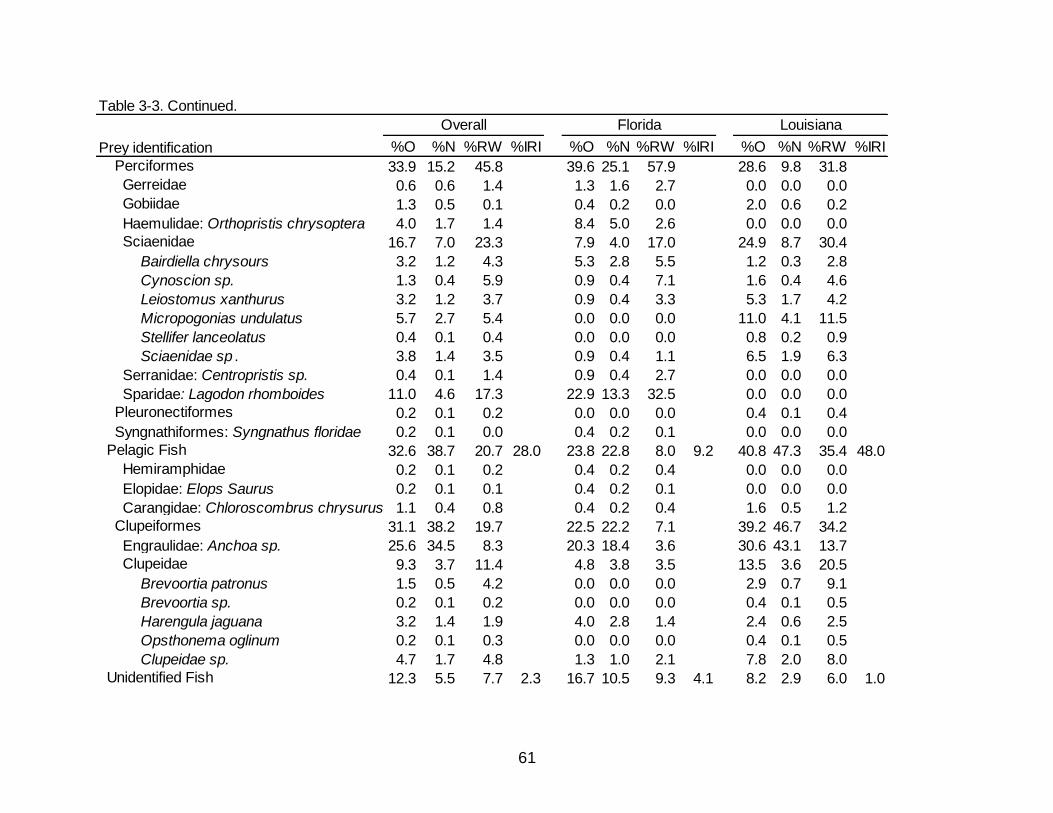
61
%O %N %RW %IRI %O %N %RW %IRI %O %N %RW %IRI
33.9 15.2 45.8 39.6 25.1 57.9 28.6 9.8 31.8
0.6 0.6 1.4 1.3 1.6 2.7 0.0 0.0 0.0
1.3 0.5 0.1 0.4 0.2 0.0 2.0 0.6 0.2
4.0 1.7 1.4 8.4 5.0 2.6 0.0 0.0 0.0
16.7 7.0 23.3 7.9 4.0 17.0 24.9 8.7 30.4
Bairdiella chrysours 3.2 1.2 4.3 5.3 2.8 5.5 1.2 0.3 2.8
Cynoscion sp. 1.3 0.4 5.9 0.9 0.4 7.1 1.6 0.4 4.6
Leiostomus xanthurus 3.2 1.2 3.7 0.9 0.4 3.3 5.3 1.7 4.2
Micropogonias undulatus 5.7 2.7 5.4 0.0 0.0 0.0 11.0 4.1 11.5
Stellifer lanceolatus 0.4 0.1 0.4 0.0 0.0 0.0 0.8 0.2 0.9
Sciaenidae sp . 3.8 1.4 3.5 0.9 0.4 1.1 6.5 1.9 6.3
0.4 0.1 1.4 0.9 0.4 2.7 0.0 0.0 0.0
11.0 4.6 17.3 22.9 13.3 32.5 0.0 0.0 0.0
0.2 0.1 0.2 0.0 0.0 0.0 0.4 0.1 0.4
0.2 0.1 0.0 0.4 0.2 0.1 0.0 0.0 0.0
32.6 38.7 20.7 28.0 23.8 22.8 8.0 9.2 40.8 47.3 35.4 48.0
0.2 0.1 0.2 0.4 0.2 0.4 0.0 0.0 0.0
0.2 0.1 0.1 0.4 0.2 0.1 0.0 0.0 0.0
1.1 0.4 0.8 0.4 0.2 0.4 1.6 0.5 1.2
31.1 38.2 19.7 22.5 22.2 7.1 39.2 46.7 34.2
25.6 34.5 8.3 20.3 18.4 3.6 30.6 43.1 13.7
9.3 3.7 11.4 4.8 3.8 3.5 13.5 3.6 20.5
Brevoortia patronus 1.5 0.5 4.2 0.0 0.0 0.0 2.9 0.7 9.1
Brevoortia sp. 0.2 0.1 0.2 0.0 0.0 0.0 0.4 0.1 0.5
Harengula jaguana 3.2 1.4 1.9 4.0 2.8 1.4 2.4 0.6 2.5
Opsthonema oglinum 0.2 0.1 0.3 0.0 0.0 0.0 0.4 0.1 0.5
Clupeidae sp. 4.7 1.7 4.8 1.3 1.0 2.1 7.8 2.0 8.0
12.3 5.5 7.7 2.3 16.7 10.5 9.3 4.1 8.2 2.9 6.0 1.0
Prey identification
Florida Louisiana
Engraulidae: Anchoa sp.
Clupeidae
Unidentified Fish
Syngnathiformes: Syngnathus floridae
Pelagic Fish
Hemiramphidae
Elopidae: Elops Saurus
Carangidae: Chloroscombrus chrysurus
Clupeiformes
Pleuronectiformes
Perciformes
Gerreidae
Overall
Table 3-3. Continued.
Gobiidae
Haemulidae: Orthopristis chrysoptera
Sciaenidae
Serranidae: Centropristis sp.
Sparidae: Lagodon rhomboides
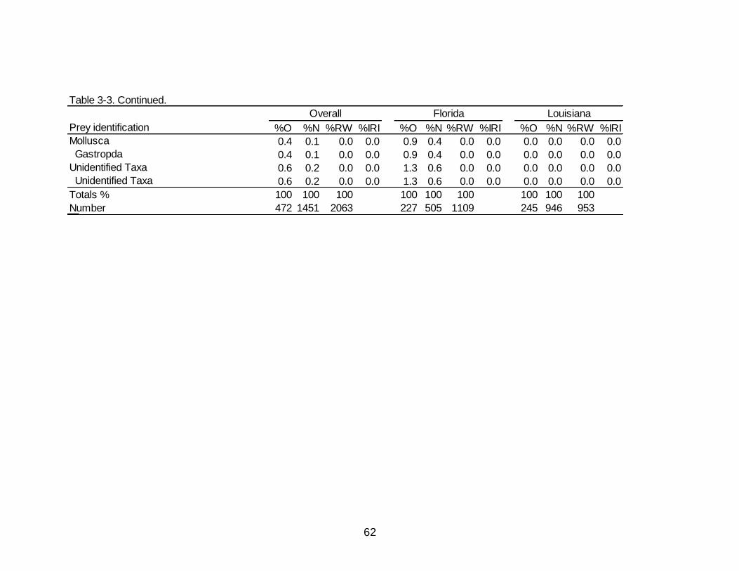
62
%O %N %RW %IRI %O %N %RW %IRI %O %N %RW %IRI
0.4 0.1 0.0 0.0 0.9 0.4 0.0 0.0 0.0 0.0 0.0 0.0
0.4 0.1 0.0 0.0 0.9 0.4 0.0 0.0 0.0 0.0 0.0 0.0
0.6 0.2 0.0 0.0 1.3 0.6 0.0 0.0 0.0 0.0 0.0 0.0
0.6 0.2 0.0 0.0 1.3 0.6 0.0 0.0 0.0 0.0 0.0 0.0
Totals % 100 100 100 100 100 100 100 100 100
Number 472 1451 2063 227 505 1109 245 946 953
Overall Florida Louisiana
Prey identification
Mollusca
Gastropda
Unidentified Taxa
Unidentified Taxa
Table 3-3. Continued.
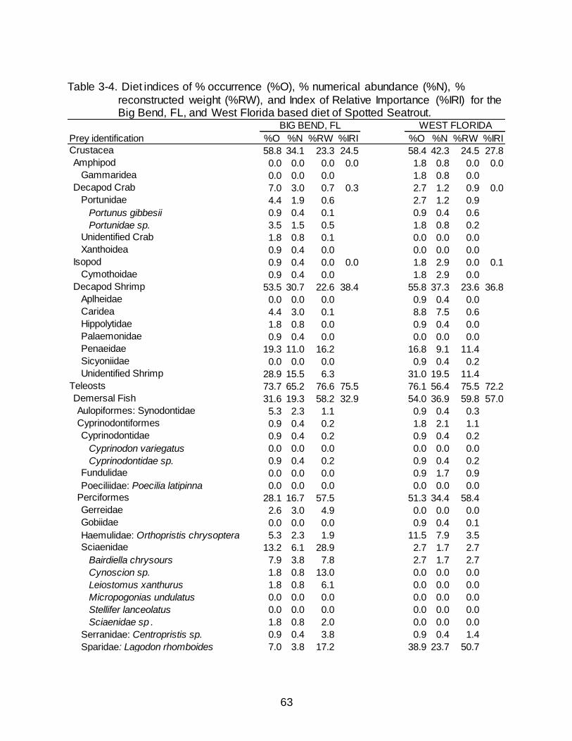
63
Table 3-4. Diet indices of % occurrence (%O), % numerical abundance (%N), %
reconstructed weight (%RW), and Index of Relative Importance (%IRI) for the Big Bend, FL, and West Florida based diet of Spotted Seatrout.
%O %N %RW %IRI %O %N %RW %IRI
58.8 34.1 23.3 24.5 58.4 42.3 24.5 27.8
0.0 0.0 0.0 0.0 1.8 0.8 0.0 0.0
0.0 0.0 0.0 1.8 0.8 0.0
7.0 3.0 0.7 0.3 2.7 1.2 0.9 0.0
4.4 1.9 0.6 2.7 1.2 0.9
Portunus gibbesii 0.9 0.4 0.1 0.9 0.4 0.6
Portunidae sp. 3.5 1.5 0.5 1.8 0.8 0.2
1.8 0.8 0.1 0.0 0.0 0.0
0.9 0.4 0.0 0.0 0.0 0.0
0.9 0.4 0.0 0.0 1.8 2.9 0.0 0.1
0.9 0.4 0.0 1.8 2.9 0.0
53.5 30.7 22.6 38.4 55.8 37.3 23.6 36.8
0.0 0.0 0.0 0.9 0.4 0.0
4.4 3.0 0.1 8.8 7.5 0.6
1.8 0.8 0.0 0.9 0.4 0.0
0.9 0.4 0.0 0.0 0.0 0.0
19.3 11.0 16.2 16.8 9.1 11.4
0.0 0.0 0.0 0.9 0.4 0.2
28.9 15.5 6.3 31.0 19.5 11.4
73.7 65.2 76.6 75.5 76.1 56.4 75.5 72.2
31.6 19.3 58.2 32.9 54.0 36.9 59.8 57.0
5.3 2.3 1.1 0.9 0.4 0.3
0.9 0.4 0.2 1.8 2.1 1.1
0.9 0.4 0.2 0.9 0.4 0.2
Cyprinodon variegatus 0.0 0.0 0.0 0.0 0.0 0.0
Cyprinodontidae sp. 0.9 0.4 0.2 0.9 0.4 0.2
0.0 0.0 0.0 0.9 1.7 0.9
0.0 0.0 0.0 0.0 0.0 0.0
28.1 16.7 57.5 51.3 34.4 58.4
2.6 3.0 4.9 0.0 0.0 0.0
0.0 0.0 0.0 0.9 0.4 0.1
5.3 2.3 1.9 11.5 7.9 3.5
13.2 6.1 28.9 2.7 1.7 2.7
Bairdiella chrysours 7.9 3.8 7.8 2.7 1.7 2.7
Cynoscion sp. 1.8 0.8 13.0 0.0 0.0 0.0
Leiostomus xanthurus 1.8 0.8 6.1 0.0 0.0 0.0
Micropogonias undulatus 0.0 0.0 0.0 0.0 0.0 0.0
Stellifer lanceolatus 0.0 0.0 0.0 0.0 0.0 0.0
Sciaenidae sp . 1.8 0.8 2.0 0.0 0.0 0.0
0.9 0.4 3.8 0.9 0.4 1.4
7.0 3.8 17.2 38.9 23.7 50.7
Serranidae: Centropristis sp.
Sparidae: Lagodon rhomboides
Poeciliidae: Poecilia latipinna
Perciformes
Gerreidae
Gobiidae
Haemulidae: Orthopristis chrysoptera
Sciaenidae
Fundulidae
Caridea
Hippolytidae
Palaemonidae
Penaeidae
Sicyoniidae
Unidentified Shrimp
Teleosts
Demersal Fish
Aulopiformes: Synodontidae
Cyprinodontiformes
Cyprinodontidae
Aplheidae
Crustacea
Amphipod
Gammaridea
Decapod Crab
Portunidae
Unidentified Crab
Xanthoidea
Isopod
Cymothoidae
Decapod Shrimp
Prey identification
BIG BEND, FL WEST FLORIDA
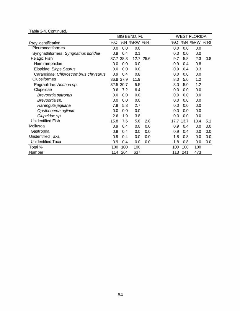
64
%O %N %RW %IRI %O %N %RW %IRI
0.0 0.0 0.0 0.0 0.0 0.0
0.9 0.4 0.1 0.0 0.0 0.0
37.7 38.3 12.7 25.6 9.7 5.8 2.3 0.8
0.0 0.0 0.0 0.9 0.4 0.8
0.0 0.0 0.0 0.9 0.4 0.3
0.9 0.4 0.8 0.0 0.0 0.0
36.8 37.9 11.9 8.0 5.0 1.2
32.5 30.7 5.5 8.0 5.0 1.2
9.6 7.2 6.4 0.0 0.0 0.0
Brevoortia patronus 0.0 0.0 0.0 0.0 0.0 0.0
Brevoortia sp. 0.0 0.0 0.0 0.0 0.0 0.0
Harengula jaguana 7.9 5.3 2.7 0.0 0.0 0.0
Opsthonema oglinum 0.0 0.0 0.0 0.0 0.0 0.0
Clupeidae sp. 2.6 1.9 3.8 0.0 0.0 0.0
15.8 7.6 5.8 2.8 17.7 13.7 13.4 5.1
0.9 0.4 0.0 0.0 0.9 0.4 0.0 0.0
0.9 0.4 0.0 0.0 0.9 0.4 0.0 0.0
0.9 0.4 0.0 0.0 1.8 0.8 0.0 0.0
0.9 0.4 0.0 0.0 1.8 0.8 0.0 0.0
100 100 100 100 100 100
114 264 637 113 241 473
BIG BEND, FL WEST FLORIDA
Unidentified Taxa
Unidentified Taxa
Total %
Pleuronectiformes
Syngnathiformes: Syngnathus floridae
Pelagic Fish
Hemiramphidae
Elopidae: Elops Saurus
Carangidae: Chloroscombrus chrysurus
Number
Clupeiformes
Engraulidae: Anchoa sp.
Clupeidae
Unidentified Fish
Mollusca
Gastropda
Table 3-4. Continued.
Prey identification
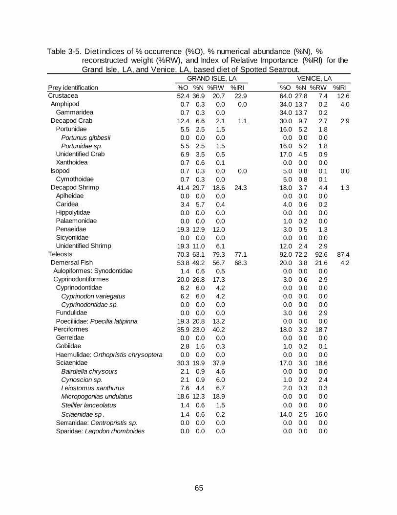
65
Table 3-5. Diet indices of % occurrence (%O), % numerical abundance (%N), % reconstructed weight (%RW), and Index of Relative Importance (%IRI) for the
Grand Isle, LA, and Venice, LA, based diet of Spotted Seatrout.
%O %N %RW %IRI %O %N %RW %IRI
52.4 36.9 20.7 22.9 64.0 27.8 7.4 12.6
0.7 0.3 0.0 0.0 34.0 13.7 0.2 4.0
0.7 0.3 0.0 34.0 13.7 0.2
12.4 6.6 2.1 1.1 30.0 9.7 2.7 2.9
5.5 2.5 1.5 16.0 5.2 1.8
Portunus gibbesii 0.0 0.0 0.0 0.0 0.0 0.0
Portunidae sp. 5.5 2.5 1.5 16.0 5.2 1.8
6.9 3.5 0.5 17.0 4.5 0.9
0.7 0.6 0.1 0.0 0.0 0.0
0.7 0.3 0.0 0.0 5.0 0.8 0.1 0.0
0.7 0.3 0.0 5.0 0.8 0.1
41.4 29.7 18.6 24.3 18.0 3.7 4.4 1.3
0.0 0.0 0.0 0.0 0.0 0.0
3.4 5.7 0.4 4.0 0.6 0.2
0.0 0.0 0.0 0.0 0.0 0.0
0.0 0.0 0.0 1.0 0.2 0.0
19.3 12.9 12.0 3.0 0.5 1.3
0.0 0.0 0.0 0.0 0.0 0.0
19.3 11.0 6.1 12.0 2.4 2.9
70.3 63.1 79.3 77.1 92.0 72.2 92.6 87.4
53.8 49.2 56.7 68.3 20.0 3.8 21.6 4.2
1.4 0.6 0.5 0.0 0.0 0.0
20.0 26.8 17.3 3.0 0.6 2.9
6.2 6.0 4.2 0.0 0.0 0.0
Cyprinodon variegatus 6.2 6.0 4.2 0.0 0.0 0.0
Cyprinodontidae sp. 0.0 0.0 0.0 0.0 0.0 0.0
0.0 0.0 0.0 3.0 0.6 2.9
19.3 20.8 13.2 0.0 0.0 0.0
35.9 23.0 40.2 18.0 3.2 18.7
0.0 0.0 0.0 0.0 0.0 0.0
2.8 1.6 0.3 1.0 0.2 0.1
0.0 0.0 0.0 0.0 0.0 0.0
30.3 19.9 37.9 17.0 3.0 18.6
Bairdiella chrysours 2.1 0.9 4.6 0.0 0.0 0.0
Cynoscion sp. 2.1 0.9 6.0 1.0 0.2 2.4
Leiostomus xanthurus 7.6 4.4 6.7 2.0 0.3 0.3
Micropogonias undulatus 18.6 12.3 18.9 0.0 0.0 0.0
Stellifer lanceolatus 1.4 0.6 1.5 0.0 0.0 0.0
Sciaenidae sp . 1.4 0.6 0.2 14.0 2.5 16.0
0.0 0.0 0.0 0.0 0.0 0.0
0.0 0.0 0.0 0.0 0.0 0.0
GRAND ISLE, LA
Perciformes
Gerreidae
Gobiidae
Haemulidae: Orthopristis chrysoptera
Sciaenidae
Teleosts
Demersal Fish
Serranidae: Centropristis sp.
Sparidae: Lagodon rhomboides
Poeciliidae: Poecilia latipinna
Aulopiformes: Synodontidae
Cyprinodontiformes
Cyprinodontidae
Fundulidae
Caridea
Hippolytidae
Palaemonidae
Penaeidae
Sicyoniidae
Unidentified Shrimp
Prey identification
Aplheidae
Crustacea
Amphipod
Gammaridea
Decapod Crab
Portunidae
Unidentified Crab
Xanthoidea
Isopod
Cymothoidae
Decapod Shrimp
VENICE, LA
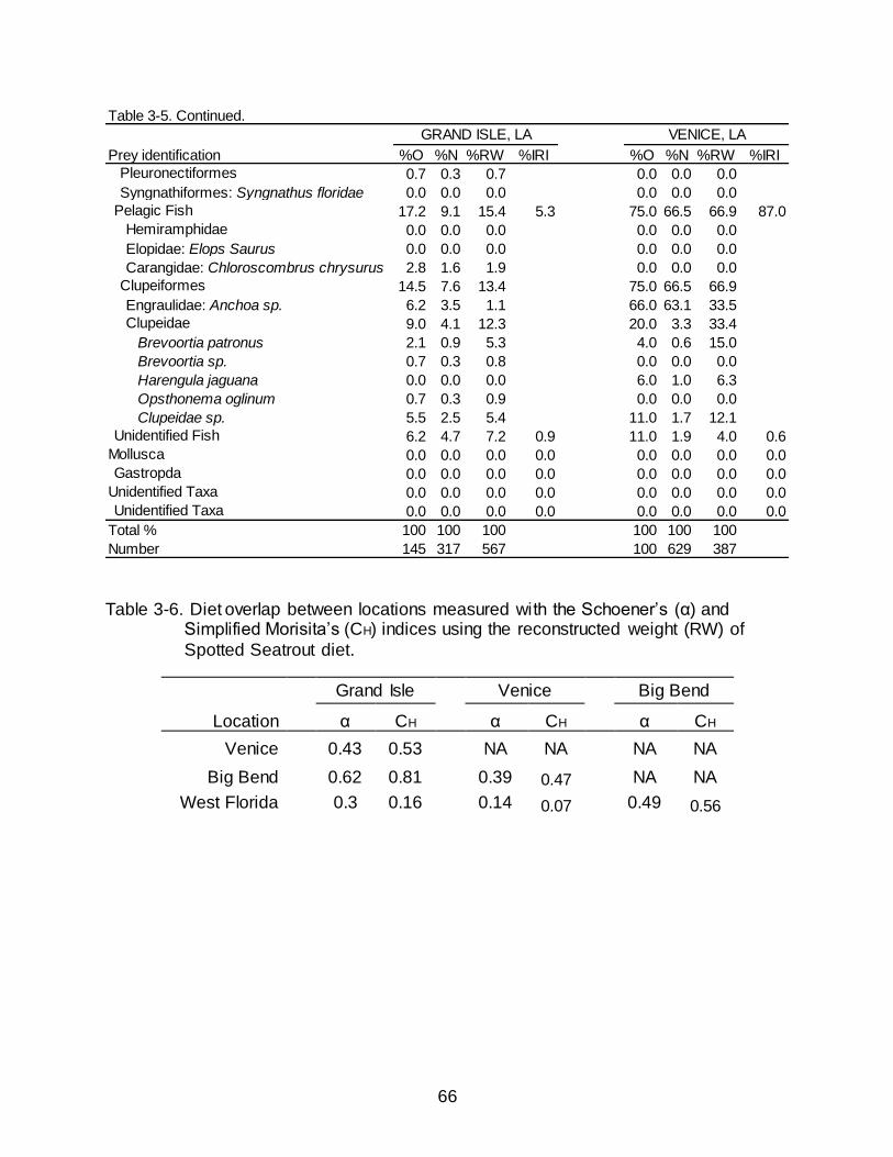
66
Table 3-6. Diet overlap between locations measured with the Schoener’s (α) and
Simplified Morisita’s (CH) indices using the reconstructed weight (RW) of
Spotted Seatrout diet.
Location
Grand Isle Venice Big Bend
α CH α CH α CH
Venice 0.43 0.53 NA NA NA NA
Big Bend 0.62 0.81 0.39 0.47 NA NA
West Florida 0.3 0.16 0.14 0.07 0.49 0.56
%O %N %RW %IRI %O %N %RW %IRI
0.7 0.3 0.7 0.0 0.0 0.0
0.0 0.0 0.0 0.0 0.0 0.0
17.2 9.1 15.4 5.3 75.0 66.5 66.9 87.0
0.0 0.0 0.0 0.0 0.0 0.0
0.0 0.0 0.0 0.0 0.0 0.0
2.8 1.6 1.9 0.0 0.0 0.0
14.5 7.6 13.4 75.0 66.5 66.9
6.2 3.5 1.1 66.0 63.1 33.5
9.0 4.1 12.3 20.0 3.3 33.4
Brevoortia patronus 2.1 0.9 5.3 4.0 0.6 15.0
Brevoortia sp. 0.7 0.3 0.8 0.0 0.0 0.0
Harengula jaguana 0.0 0.0 0.0 6.0 1.0 6.3
Opsthonema oglinum 0.7 0.3 0.9 0.0 0.0 0.0
Clupeidae sp. 5.5 2.5 5.4 11.0 1.7 12.1
6.2 4.7 7.2 0.9 11.0 1.9 4.0 0.6
0.0 0.0 0.0 0.0 0.0 0.0 0.0 0.0
0.0 0.0 0.0 0.0 0.0 0.0 0.0 0.0
0.0 0.0 0.0 0.0 0.0 0.0 0.0 0.0
0.0 0.0 0.0 0.0 0.0 0.0 0.0 0.0
100 100 100 100 100 100
145 317 567 100 629 387
Unidentified Taxa
Unidentified Taxa
Total %
Number
Clupeidae
Unidentified Fish
Mollusca
Gastropda
Table 3-5. Continued.
Prey identification
GRAND ISLE, LA VENICE, LA
Clupeiformes
Engraulidae: Anchoa sp.
Pleuronectiformes
Syngnathiformes: Syngnathus floridae
Pelagic Fish
Hemiramphidae
Elopidae: Elops Saurus
Carangidae: Chloroscombrus chrysurus
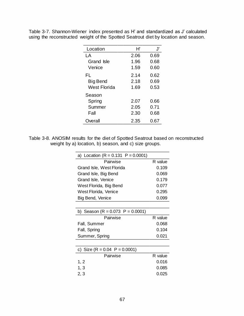
67
Table 3-7. Shannon-Wiener index presented as H’ and standardized as J’ calculated using the reconstructed weight of the Spotted Seatrout diet by location and season.
Location H' J'
LA 2.06 0.69
Grand Isle 1.96 0.68
Venice 1.59 0.60
FL 2.14 0.62
Big Bend 2.18 0.69
West Florida 1.69 0.53
Season
Spring 2.07 0.66
Summer 2.05 0.71
Fall 2.30 0.68
Overall 2.35 0.67
Table 3-8. ANOSIM results for the diet of Spotted Seatrout based on reconstructed
weight by a) location, b) season, and c) size groups.
a) Location (R = 0.131 P = 0.0001)
Pairwise R value
Grand Isle, West Florida 0.109
Grand Isle, Big Bend 0.069
Grand Isle, Venice 0.179
West Florida, Big Bend 0.077
West Florida, Venice 0.295
Big Bend, Venice 0.099
b) Season (R = 0.073 P = 0.0001)
Pairwise R value
Fall, Summer 0.068
Fall, Spring 0.104
Summer, Spring 0.021
c) Size (R = 0.04 P = 0.0001)
Pairwise R value
1, 2 0.016
1, 3 0.085
2, 3 0.025
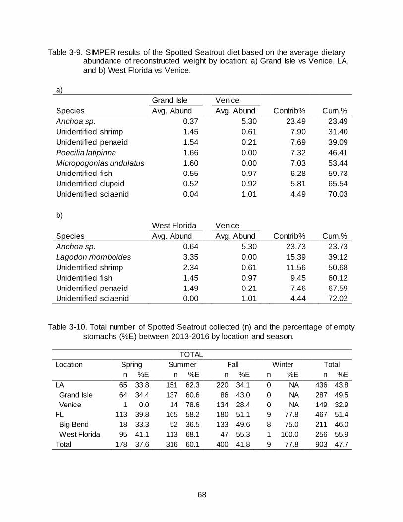
68
Table 3-9. SIMPER results of the Spotted Seatrout diet based on the average dietary abundance of reconstructed weight by location: a) Grand Isle vs Venice, LA,
and b) West Florida vs Venice.
a)
Grand Isle Venice
Species Avg. Abund Avg. Abund Contrib% Cum.%
Anchoa sp. 0.37 5.30 23.49 23.49
Unidentified shrimp 1.45 0.61 7.90 31.40
Unidentified penaeid 1.54 0.21 7.69 39.09
Poecilia latipinna 1.66 0.00 7.32 46.41
Micropogonias undulatus 1.60 0.00 7.03 53.44
Unidentified fish 0.55 0.97 6.28 59.73
Unidentified clupeid 0.52 0.92 5.81 65.54
Unidentified sciaenid 0.04 1.01 4.49 70.03
b)
West Florida Venice
Species Avg. Abund Avg. Abund Contrib% Cum.%
Anchoa sp. 0.64 5.30 23.73 23.73
Lagodon rhomboides 3.35 0.00 15.39 39.12
Unidentified shrimp 2.34 0.61 11.56 50.68
Unidentified fish 1.45 0.97 9.45 60.12
Unidentified penaeid 1.49 0.21 7.46 67.59
Unidentified sciaenid 0.00 1.01 4.44 72.02
Table 3-10. Total number of Spotted Seatrout collected (n) and the percentage of empty
stomachs (%E) between 2013-2016 by location and season.
TOTAL
Location Spring Summer Fall Winter Total
n %E n %E n %E n %E n %E
LA 65 33.8 151 62.3 220 34.1 0 NA 436 43.8
Grand Isle 64 34.4 137 60.6 86 43.0 0 NA 287 49.5
Venice 1 0.0 14 78.6 134 28.4 0 NA 149 32.9
FL 113 39.8 165 58.2 180 51.1 9 77.8 467 51.4
Big Bend 18 33.3 52 36.5 133 49.6 8 75.0 211 46.0
West Florida 95 41.1 113 68.1 47 55.3 1 100.0 256 55.9
Total 178 37.6 316 60.1 400 41.8 9 77.8 903 47.7
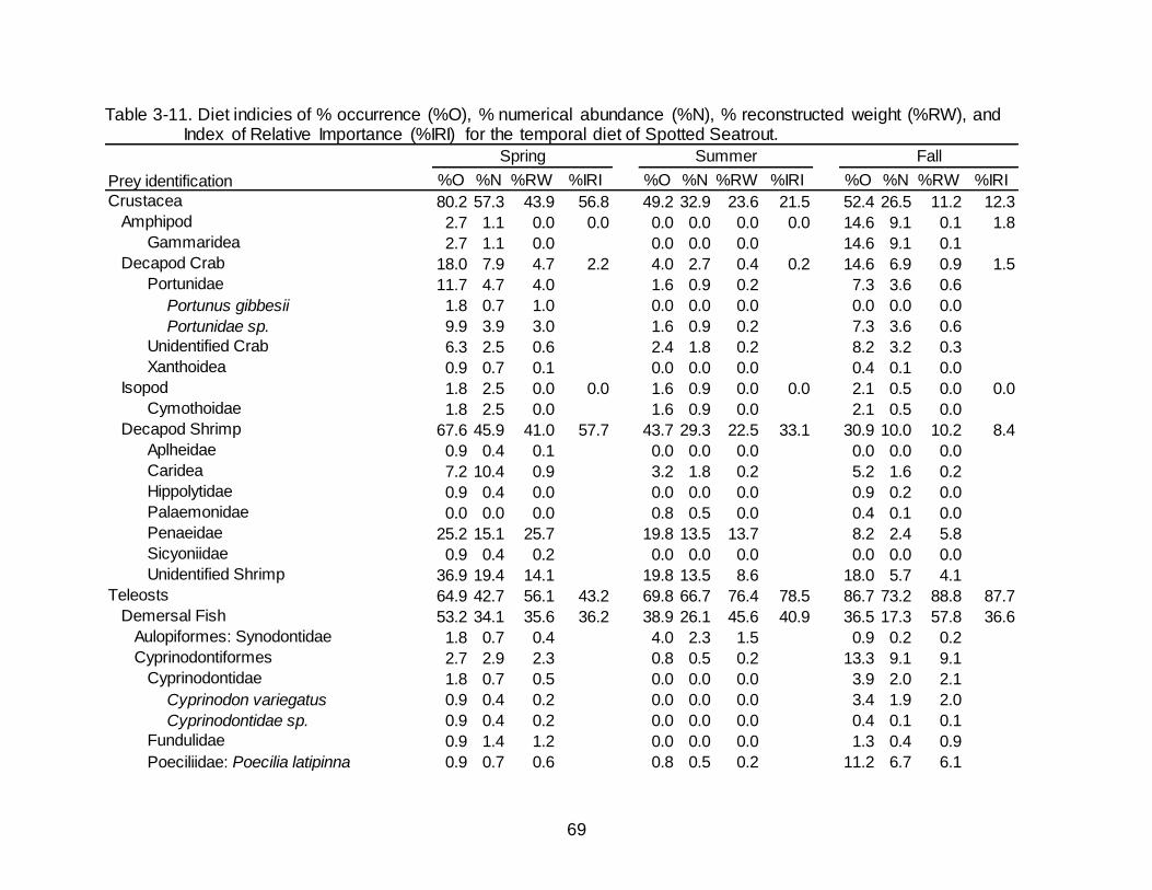
69
Table 3-11. Diet indicies of % occurrence (%O), % numerical abundance (%N), % reconstructed weight (%RW), and Index of Relative Importance (%IRI) for the temporal diet of Spotted Seatrout.
%O %N %RW %IRI %O %N %RW %IRI %O %N %RW %IRI
80.2 57.3 43.9 56.8 49.2 32.9 23.6 21.5 52.4 26.5 11.2 12.3
2.7 1.1 0.0 0.0 0.0 0.0 0.0 0.0 14.6 9.1 0.1 1.8
2.7 1.1 0.0 0.0 0.0 0.0 14.6 9.1 0.1
18.0 7.9 4.7 2.2 4.0 2.7 0.4 0.2 14.6 6.9 0.9 1.5
11.7 4.7 4.0 1.6 0.9 0.2 7.3 3.6 0.6
Portunus gibbesii 1.8 0.7 1.0 0.0 0.0 0.0 0.0 0.0 0.0
Portunidae sp. 9.9 3.9 3.0 1.6 0.9 0.2 7.3 3.6 0.6
6.3 2.5 0.6 2.4 1.8 0.2 8.2 3.2 0.3
0.9 0.7 0.1 0.0 0.0 0.0 0.4 0.1 0.0
1.8 2.5 0.0 0.0 1.6 0.9 0.0 0.0 2.1 0.5 0.0 0.0
1.8 2.5 0.0 1.6 0.9 0.0 2.1 0.5 0.0
67.6 45.9 41.0 57.7 43.7 29.3 22.5 33.1 30.9 10.0 10.2 8.4
0.9 0.4 0.1 0.0 0.0 0.0 0.0 0.0 0.0
7.2 10.4 0.9 3.2 1.8 0.2 5.2 1.6 0.2
0.9 0.4 0.0 0.0 0.0 0.0 0.9 0.2 0.0
0.0 0.0 0.0 0.8 0.5 0.0 0.4 0.1 0.0
25.2 15.1 25.7 19.8 13.5 13.7 8.2 2.4 5.8
0.9 0.4 0.2 0.0 0.0 0.0 0.0 0.0 0.0
36.9 19.4 14.1 19.8 13.5 8.6 18.0 5.7 4.1
64.9 42.7 56.1 43.2 69.8 66.7 76.4 78.5 86.7 73.2 88.8 87.7
53.2 34.1 35.6 36.2 38.9 26.1 45.6 40.9 36.5 17.3 57.8 36.6
1.8 0.7 0.4 4.0 2.3 1.5 0.9 0.2 0.2
2.7 2.9 2.3 0.8 0.5 0.2 13.3 9.1 9.1
1.8 0.7 0.5 0.0 0.0 0.0 3.9 2.0 2.1
Cyprinodon variegatus 0.9 0.4 0.2 0.0 0.0 0.0 3.4 1.9 2.0
Cyprinodontidae sp. 0.9 0.4 0.2 0.0 0.0 0.0 0.4 0.1 0.1
0.9 1.4 1.2 0.0 0.0 0.0 1.3 0.4 0.9
0.9 0.7 0.6 0.8 0.5 0.2 11.2 6.7 6.1
Aulopiformes: Synodontidae
Cyprinodontiformes
Cyprinodontidae
Fundulidae
Poeciliidae: Poecilia latipinna
Demersal Fish
Isopod
Cymothoidae
Decapod Shrimp
Aplheidae
Caridea
Hippolytidae
Palaemonidae
Penaeidae
Sicyoniidae
Unidentified Shrimp
Teleosts
Xanthoidea
Spring Summer Fall
Crustacea
Prey identification
Amphipod
Gammaridea
Decapod Crab
Portunidae
Unidentified Crab
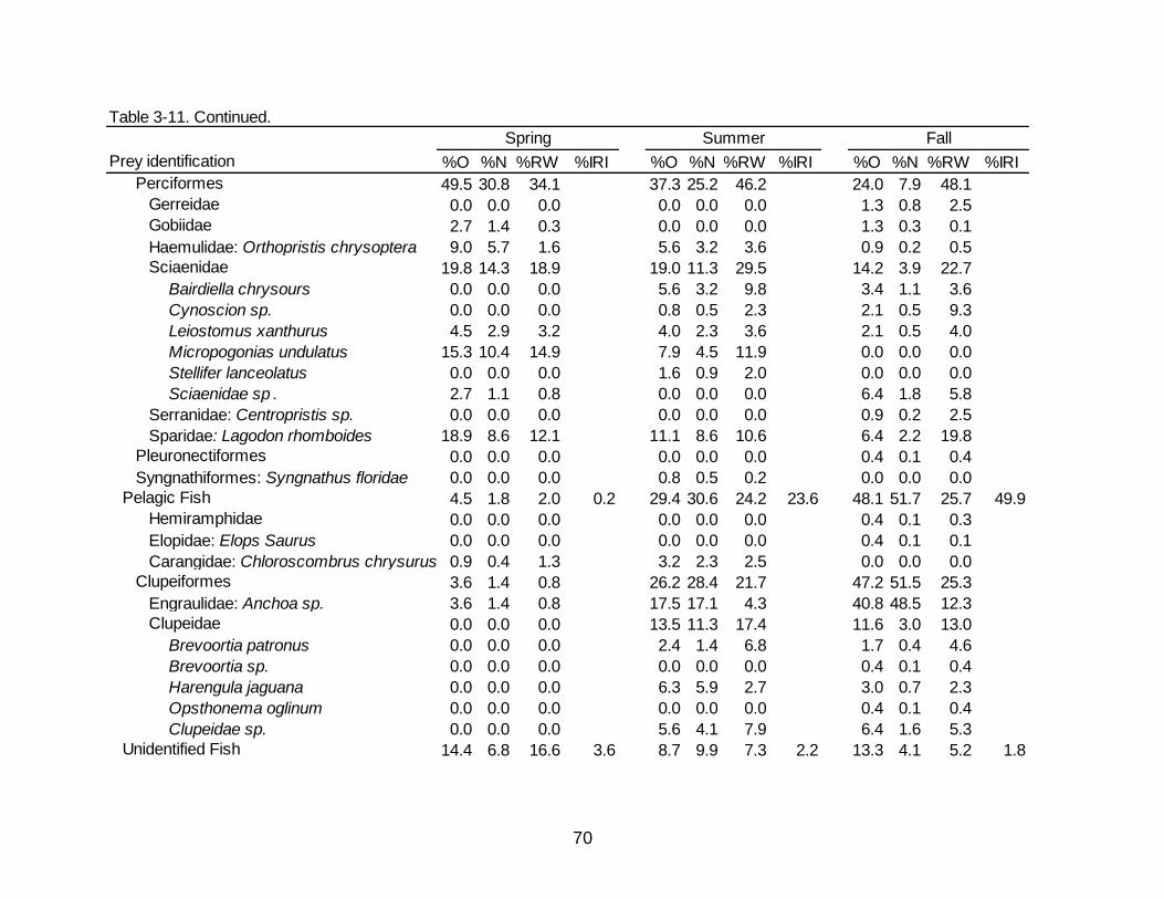
70
%O %N %RW %IRI %O %N %RW %IRI %O %N %RW %IRI
49.5 30.8 34.1 37.3 25.2 46.2 24.0 7.9 48.1
0.0 0.0 0.0 0.0 0.0 0.0 1.3 0.8 2.5
2.7 1.4 0.3 0.0 0.0 0.0 1.3 0.3 0.1
9.0 5.7 1.6 5.6 3.2 3.6 0.9 0.2 0.5
19.8 14.3 18.9 19.0 11.3 29.5 14.2 3.9 22.7
Bairdiella chrysours 0.0 0.0 0.0 5.6 3.2 9.8 3.4 1.1 3.6
Cynoscion sp. 0.0 0.0 0.0 0.8 0.5 2.3 2.1 0.5 9.3
Leiostomus xanthurus 4.5 2.9 3.2 4.0 2.3 3.6 2.1 0.5 4.0
Micropogonias undulatus 15.3 10.4 14.9 7.9 4.5 11.9 0.0 0.0 0.0
Stellifer lanceolatus 0.0 0.0 0.0 1.6 0.9 2.0 0.0 0.0 0.0
Sciaenidae sp . 2.7 1.1 0.8 0.0 0.0 0.0 6.4 1.8 5.8
0.0 0.0 0.0 0.0 0.0 0.0 0.9 0.2 2.5
18.9 8.6 12.1 11.1 8.6 10.6 6.4 2.2 19.8
0.0 0.0 0.0 0.0 0.0 0.0 0.4 0.1 0.4
0.0 0.0 0.0 0.8 0.5 0.2 0.0 0.0 0.0
4.5 1.8 2.0 0.2 29.4 30.6 24.2 23.6 48.1 51.7 25.7 49.9
0.0 0.0 0.0 0.0 0.0 0.0 0.4 0.1 0.3
0.0 0.0 0.0 0.0 0.0 0.0 0.4 0.1 0.1
0.9 0.4 1.3 3.2 2.3 2.5 0.0 0.0 0.0
3.6 1.4 0.8 26.2 28.4 21.7 47.2 51.5 25.3
3.6 1.4 0.8 17.5 17.1 4.3 40.8 48.5 12.3
0.0 0.0 0.0 13.5 11.3 17.4 11.6 3.0 13.0
Brevoortia patronus 0.0 0.0 0.0 2.4 1.4 6.8 1.7 0.4 4.6
Brevoortia sp. 0.0 0.0 0.0 0.0 0.0 0.0 0.4 0.1 0.4
Harengula jaguana 0.0 0.0 0.0 6.3 5.9 2.7 3.0 0.7 2.3
Opsthonema oglinum 0.0 0.0 0.0 0.0 0.0 0.0 0.4 0.1 0.4
Clupeidae sp. 0.0 0.0 0.0 5.6 4.1 7.9 6.4 1.6 5.3
14.4 6.8 16.6 3.6 8.7 9.9 7.3 2.2 13.3 4.1 5.2 1.8
Engraulidae: Anchoa sp.
Clupeidae
Unidentified Fish
Clupeiformes
Gobiidae
Haemulidae: Orthopristis chrysoptera
Sciaenidae
Serranidae: Centropristis sp.
Sparidae: Lagodon rhomboides
Pleuronectiformes
Syngnathiformes: Syngnathus floridae
Pelagic Fish
Hemiramphidae
Elopidae: Elops Saurus
Carangidae: Chloroscombrus chrysurus
Spring Summer Fall
Prey identification
Perciformes
Gerreidae
Table 3-11. Continued.
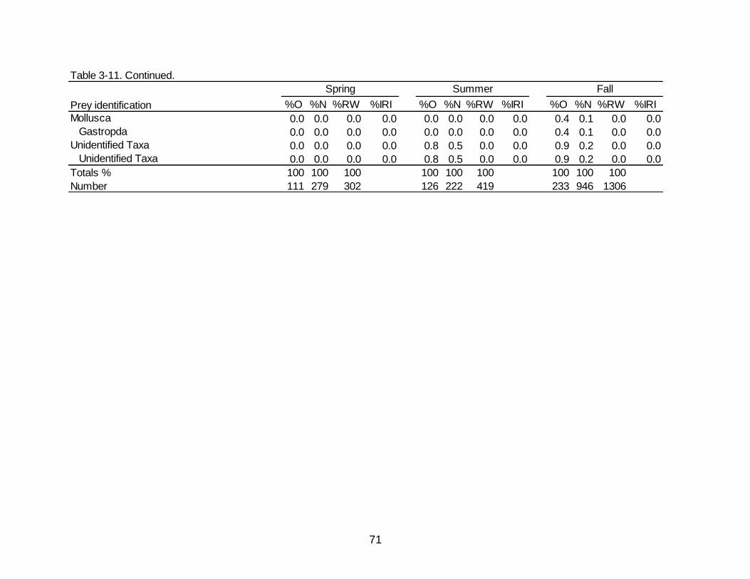
71
%O %N %RW %IRI %O %N %RW %IRI %O %N %RW %IRI
0.0 0.0 0.0 0.0 0.0 0.0 0.0 0.0 0.4 0.1 0.0 0.0
0.0 0.0 0.0 0.0 0.0 0.0 0.0 0.0 0.4 0.1 0.0 0.0
0.0 0.0 0.0 0.0 0.8 0.5 0.0 0.0 0.9 0.2 0.0 0.0
0.0 0.0 0.0 0.0 0.8 0.5 0.0 0.0 0.9 0.2 0.0 0.0
Totals % 100 100 100 100 100 100 100 100 100
Number 111 279 302 126 222 419 233 946 1306
Fall
Mollusca
Gastropda
Unidentified Taxa
Unidentified Taxa
Prey identification
Summer
Table 3-11. Continued.
Spring
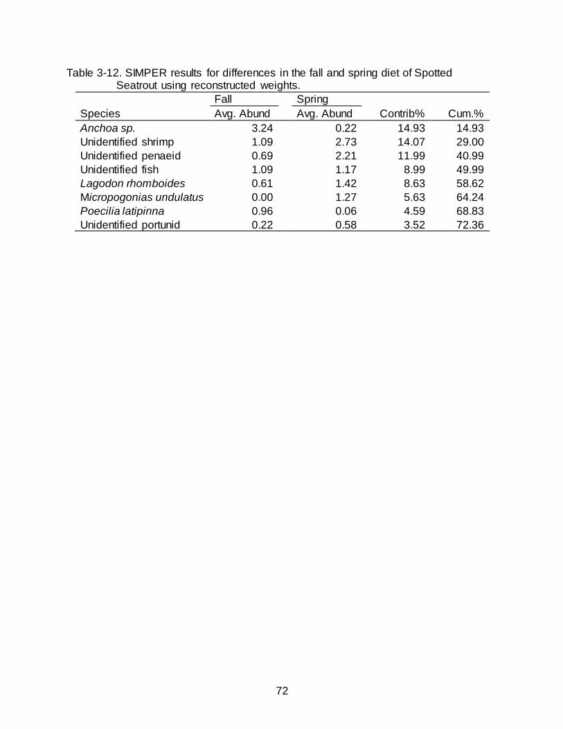
72
Table 3-12. SIMPER results for differences in the fall and spring diet of Spotted Seatrout using reconstructed weights.
Fall Spring
Species Avg. Abund Avg. Abund Contrib% Cum.%
Anchoa sp. 3.24 0.22 14.93 14.93
Unidentified shrimp 1.09 2.73 14.07 29.00
Unidentified penaeid 0.69 2.21 11.99 40.99
Unidentified fish 1.09 1.17 8.99 49.99
Lagodon rhomboides 0.61 1.42 8.63 58.62
Micropogonias undulatus 0.00 1.27 5.63 64.24
Poecilia latipinna 0.96 0.06 4.59 68.83
Unidentified portunid 0.22 0.58 3.52 72.36
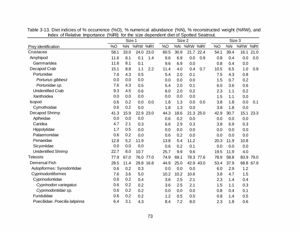
73
Table 3-13. Diet indicies of % occurrence (%O), % numerical abundance (%N), % reconstructed weight (%RW), and Index of Relative Importance (%IRI) for the size dependent diet of Spotted Seatrout.
%O %N %RW %IRI %O %N %RW %IRI %O %N %RW %IRI
58.1 33.0 24.0 23.0 60.5 30.9 21.7 22.4 54.1 39.4 16.1 21.0
11.6 8.1 0.1 1.4 9.6 6.9 0.0 0.9 0.8 0.4 0.0 0.0
11.6 8.1 0.1 9.6 6.9 0.0 0.8 0.4 0.0
15.1 8.8 1.1 2.2 11.4 4.0 0.4 0.7 10.5 6.5 1.0 0.9
7.6 4.3 0.5 5.4 2.0 0.1 7.5 4.3 0.8
Portunus gibbesii 0.0 0.0 0.0 0.0 0.0 0.0 1.5 0.7 0.2
Portunidae sp. 7.6 4.3 0.5 5.4 2.0 0.1 6.0 3.6 0.6
9.3 4.5 0.6 6.0 2.0 0.2 2.3 1.1 0.2
0.0 0.0 0.0 0.0 0.0 0.0 1.5 1.1 0.0
0.6 0.2 0.0 0.0 1.8 1.3 0.0 0.0 3.8 1.8 0.0 0.1
0.6 0.2 0.0 1.8 1.3 0.0 3.8 1.8 0.0
41.3 15.9 22.9 23.0 44.3 18.6 21.3 25.0 42.9 30.7 15.1 23.3
0.0 0.0 0.0 0.6 0.2 0.0 0.0 0.0 0.0
4.7 2.1 0.3 6.6 2.9 0.3 3.8 6.9 0.3
1.7 0.5 0.0 0.0 0.0 0.0 0.0 0.0 0.0
0.6 0.2 0.0 0.6 0.2 0.0 0.0 0.0 0.0
12.8 5.2 11.9 13.8 5.4 11.2 20.3 11.9 10.8
0.0 0.0 0.0 0.6 0.2 0.1 0.0 0.0 0.0
22.7 8.0 10.7 25.7 9.9 9.6 19.5 11.9 4.0
77.9 67.0 76.0 77.0 74.9 69.1 78.3 77.6 78.9 58.8 83.9 79.0
28.5 11.4 29.8 16.8 44.9 25.0 42.9 43.0 53.4 37.9 68.8 67.9
0.6 0.2 0.3 0.0 0.0 0.0 6.0 2.9 1.2
7.6 3.6 5.0 10.2 10.2 10.6 3.8 4.7 1.5
0.6 0.2 0.4 3.6 2.5 2.1 2.3 1.4 0.4
Cyprinodon variegatus 0.6 0.2 0.2 3.6 2.5 2.1 1.5 1.1 0.3
Cyprinodontidae sp. 0.6 0.2 0.2 0.0 0.0 0.0 0.8 0.4 0.1
0.6 0.2 0.2 1.2 0.5 0.5 0.8 1.4 0.5
6.4 3.1 4.3 8.4 7.2 8.0 2.3 1.8 0.6
Size 3
Poeciliidae: Poecilia latipinna
Hippolytidae
Palaemonidae
Penaeidae
Sicyoniidae
Unidentified Shrimp
Teleosts
Demersal Fish
Aulopiformes: Synodontidae
Cyprinodontiformes
Cyprinodontidae
Fundulidae
Caridea
Crustacea
Amphipod
Gammaridea
Decapod Crab
Portunidae
Unidentified Crab
Xanthoidea
Isopod
Cymothoidae
Decapod Shrimp
Aplheidae
Prey identification
Size 1 Size 2
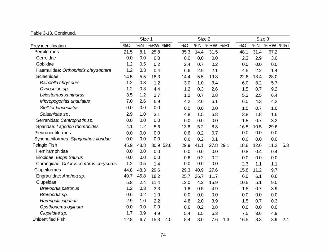
74
%O %N %RW %IRI %O %N %RW %IRI %O %N %RW %IRI
21.5 8.1 25.8 35.3 14.4 31.5 48.1 31.4 67.2
0.0 0.0 0.0 0.0 0.0 0.0 2.3 2.9 3.0
1.2 0.5 0.2 2.4 0.7 0.2 0.0 0.0 0.0
1.2 0.3 0.4 6.6 2.9 2.1 4.5 2.2 1.4
14.5 5.5 18.3 14.4 5.5 19.8 22.6 13.4 28.0
Bairdiella chrysours 1.2 0.3 1.2 3.0 1.0 3.4 6.0 3.2 5.7
Cynoscion sp. 1.2 0.3 4.4 1.2 0.3 2.6 1.5 0.7 9.2
Leiostomus xanthurus 3.5 1.2 2.7 1.2 0.7 0.8 5.3 2.5 6.4
Micropogonias undulatus 7.0 2.6 6.9 4.2 2.0 6.1 6.0 4.3 4.2
Stellifer lanceolatus 0.0 0.0 0.0 0.0 0.0 0.0 1.5 0.7 1.0
Sciaenidae sp . 2.9 1.0 3.1 4.8 1.5 6.8 3.8 1.8 1.6
0.0 0.0 0.0 0.0 0.0 0.0 1.5 0.7 3.2
4.1 1.2 5.6 13.8 5.2 8.8 16.5 10.5 29.6
0.0 0.0 0.0 0.6 0.2 0.7 0.0 0.0 0.0
0.0 0.0 0.0 0.6 0.2 0.1 0.0 0.0 0.0
45.9 48.8 30.9 52.6 29.9 41.1 27.8 29.1 18.8 12.6 11.2 5.3
0.0 0.0 0.0 0.0 0.0 0.0 0.8 0.4 0.4
0.0 0.0 0.0 0.6 0.2 0.2 0.0 0.0 0.0
1.2 0.5 1.4 0.0 0.0 0.0 2.3 1.1 1.1
44.8 48.3 29.6 29.3 40.9 27.6 15.8 11.2 9.7
40.7 45.8 18.2 25.7 36.7 11.7 6.0 6.1 0.6
5.8 2.4 11.4 12.0 4.2 15.9 10.5 5.1 9.0
Brevoortia patronus 1.2 0.3 3.3 1.8 0.5 4.9 1.5 0.7 3.9
Brevoortia sp. 0.6 0.2 1.0 0.0 0.0 0.0 0.0 0.0 0.0
Harengula jaguana 2.9 1.0 2.2 4.8 2.0 3.9 1.5 0.7 0.3
Opsthonema oglinum 0.0 0.0 0.0 0.6 0.2 0.8 0.0 0.0 0.0
Clupeidae sp. 1.7 0.9 4.9 5.4 1.5 6.3 7.5 3.6 4.9
12.8 6.7 15.3 4.0 8.4 3.0 7.6 1.3 16.5 8.3 3.9 2.4
Size 3
Engraulidae: Anchoa sp.
Clupeidae
Unidentified Fish
Syngnathiformes: Syngnathus floridae
Pelagic Fish
Hemiramphidae
Elopidae: Elops Saurus
Carangidae: Chloroscombrus chrysurus
Clupeiformes
Sparidae: Lagodon rhomboides
Table 3-13. Continued.
Prey identification
Size 1 Size 2
Pleuronectiformes
Perciformes
Gerreidae
Gobiidae
Haemulidae: Orthopristis chrysoptera
Sciaenidae
Serranidae: Centropristis sp.
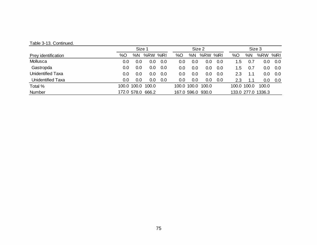
75
%O %N %RW %IRI %O %N %RW %IRI %O %N %RW %IRI
0.0 0.0 0.0 0.0 0.0 0.0 0.0 0.0 1.5 0.7 0.0 0.0
0.0 0.0 0.0 0.0 0.0 0.0 0.0 0.0 1.5 0.7 0.0 0.0
0.0 0.0 0.0 0.0 0.0 0.0 0.0 0.0 2.3 1.1 0.0 0.0
0.0 0.0 0.0 0.0 0.0 0.0 0.0 0.0 2.3 1.1 0.0 0.0
100.0 100.0 100.0 100.0 100.0 100.0 100.0 100.0 100.0
172.0 578.0 666.2 167.0 596.0 930.0 133.0 277.0 1336.3
Table 3-13. Continued.
Prey identification
Size 1 Size 2 Size 3
Unidentified Taxa
Total %
Number
Mollusca
Gastropda
Unidentified Taxa
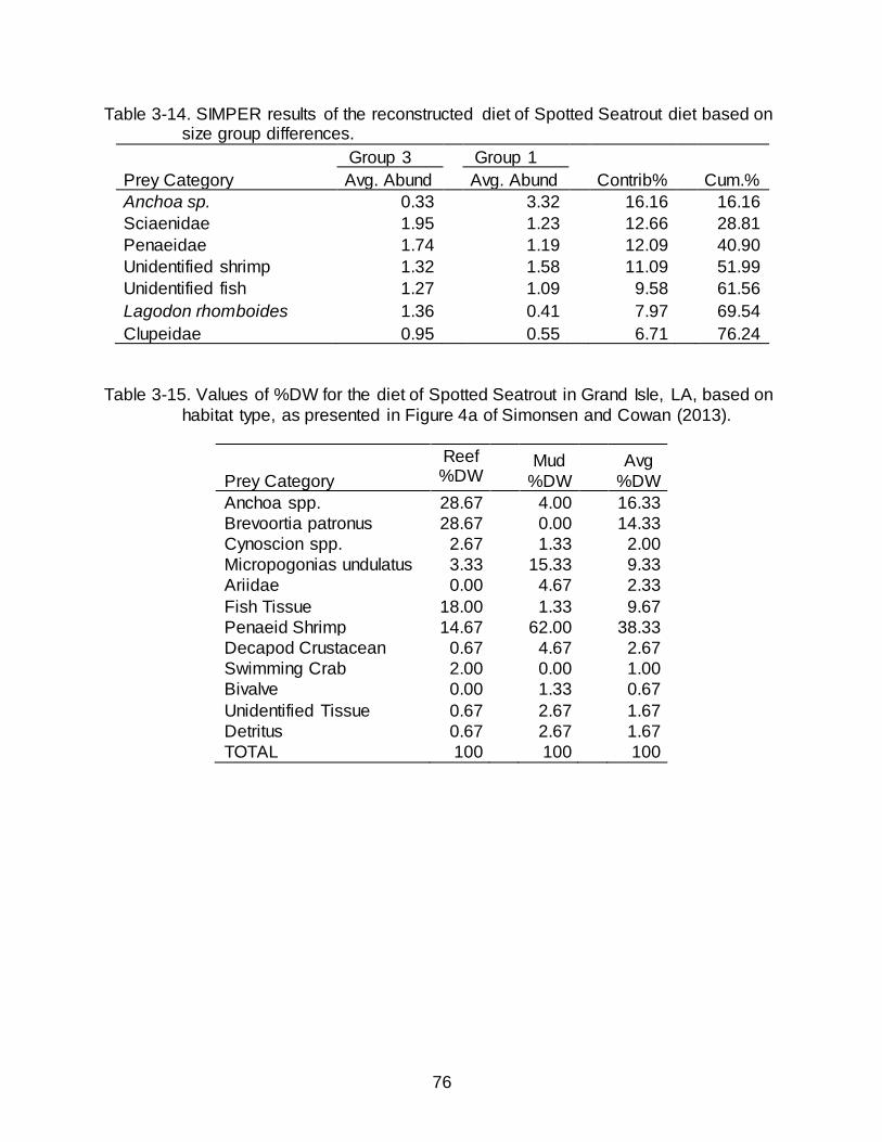
76
Table 3-14. SIMPER results of the reconstructed diet of Spotted Seatrout diet based on size group differences.
Group 3 Group 1
Prey Category Avg. Abund Avg. Abund Contrib% Cum.%
Anchoa sp. 0.33 3.32 16.16 16.16
Sciaenidae 1.95 1.23 12.66 28.81
Penaeidae 1.74 1.19 12.09 40.90
Unidentified shrimp 1.32 1.58 11.09 51.99
Unidentified fish 1.27 1.09 9.58 61.56
Lagodon rhomboides 1.36 0.41 7.97 69.54
Clupeidae 0.95 0.55 6.71 76.24
Table 3-15. Values of %DW for the diet of Spotted Seatrout in Grand Isle, LA, based on
habitat type, as presented in Figure 4a of Simonsen and Cowan (2013).
Prey Category
Reef %DW
Mud
%DW Avg
%DW
Anchoa spp. 28.67 4.00 16.33
Brevoortia patronus 28.67 0.00 14.33
Cynoscion spp. 2.67 1.33 2.00
Micropogonias undulatus 3.33 15.33 9.33
Ariidae 0.00 4.67 2.33
Fish Tissue 18.00 1.33 9.67
Penaeid Shrimp 14.67 62.00 38.33
Decapod Crustacean 0.67 4.67 2.67
Swimming Crab 2.00 0.00 1.00
Bivalve 0.00 1.33 0.67
Unidentified Tissue 0.67 2.67 1.67
Detritus 0.67 2.67 1.67
TOTAL 100 100 100
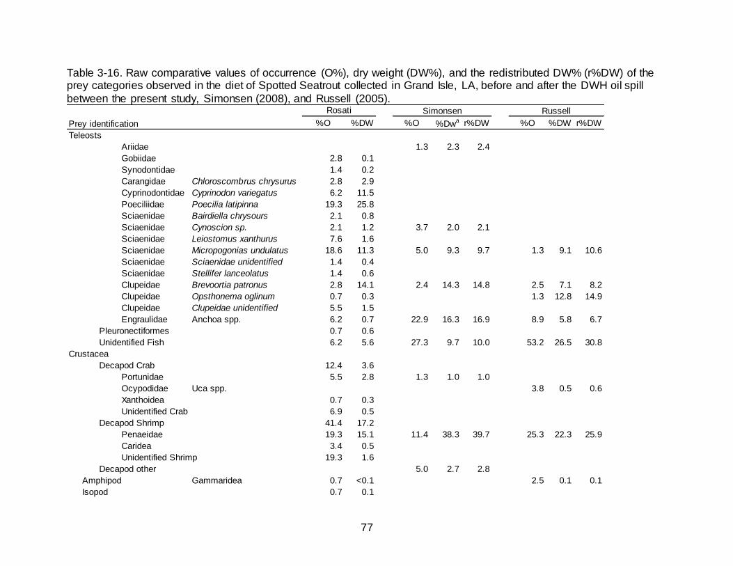
77
Table 3-16. Raw comparative values of occurrence (O%), dry weight (DW%), and the redistributed DW% (r%DW) of the prey categories observed in the diet of Spotted Seatrout collected in Grand Isle, LA, before and after the DWH oil spill
between the present study, Simonsen (2008), and Russell (2005).
%O %DW %O %Dwa r%DW %O %DW r%DW
Teleosts
Ariidae 1.3 2.3 2.4
Gobiidae 2.8 0.1
Synodontidae 1.4 0.2
Carangidae Chloroscombrus chrysurus 2.8 2.9
Cyprinodontidae Cyprinodon variegatus 6.2 11.5
Poeciliidae Poecilia latipinna 19.3 25.8
Sciaenidae Bairdiella chrysours 2.1 0.8
Sciaenidae Cynoscion sp. 2.1 1.2 3.7 2.0 2.1
Sciaenidae Leiostomus xanthurus 7.6 1.6
Sciaenidae Micropogonias undulatus 18.6 11.3 5.0 9.3 9.7 1.3 9.1 10.6
Sciaenidae Sciaenidae unidentified 1.4 0.4
Sciaenidae Stellifer lanceolatus 1.4 0.6
Clupeidae Brevoortia patronus 2.8 14.1 2.4 14.3 14.8 2.5 7.1 8.2
Clupeidae Opsthonema oglinum 0.7 0.3 1.3 12.8 14.9
Clupeidae Clupeidae unidentified 5.5 1.5
Engraulidae Anchoa spp. 6.2 0.7 22.9 16.3 16.9 8.9 5.8 6.7
Pleuronectiformes 0.7 0.6
Unidentified Fish 6.2 5.6 27.3 9.7 10.0 53.2 26.5 30.8
Crustacea
Decapod Crab 12.4 3.6
Portunidae 5.5 2.8 1.3 1.0 1.0
Ocypodidae Uca spp. 3.8 0.5 0.6
Xanthoidea 0.7 0.3
Unidentified Crab 6.9 0.5
Decapod Shrimp 41.4 17.2
Penaeidae 19.3 15.1 11.4 38.3 39.7 25.3 22.3 25.9
Caridea 3.4 0.5
Unidentified Shrimp 19.3 1.6
Decapod other 5.0 2.7 2.8
Amphipod Gammaridea 0.7 <0.1 2.5 0.1 0.1
Isopod 0.7 0.1
Prey identification
Rosati Simonsen Russell
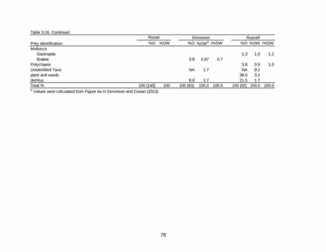
78
Table 3-16. Continued
%O %DW %O %DWb r%DW %O %DW r%DW
Mollusca
Gastropda 1.3 1.0 1.2
Bivalve 3.8 0.67 0.7
Polychaete 3.8 0.9 1.0
Unidentified Taxa NA 1.7 NA 9.1
plant and seeds 38.0 3.1
detritus 8.8 1.7 21.5 1.7
Total % 100 (145) 100 100 (83) 100.0 100.0 100 (92) 100.0 100.0a Values were calculated from Figure 4a in Simonsen and Cowan (2013)
Prey identification
Rosati Simonsen Russell
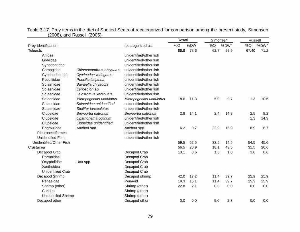
79
Table 3-17. Prey items in the diet of Spotted Seatrout recategorized for comparison among the present study, Simonsen (2008), and Russell (2005).
recategorized as: %O %DW %O %DWa %O %DWa
Teleosts 86.9 78.6 62.7 55.9 67.40 71.2
Ariidae unidentified/other fish
Gobiidae unidentified/other fish
Synodontidae unidentified/other fish
Carangidae Chloroscombrus chrysurus unidentified/other fish
Cyprinodontidae Cyprinodon variegatus unidentified/other fish
Poeciliidae Poecilia latipinna unidentified/other fish
Sciaenidae Bairdiella chrysours unidentified/other fish
Sciaenidae Cynoscion sp. unidentified/other fish
Sciaenidae Leiostomus xanthurus unidentified/other fish
Sciaenidae Micropogonias undulatus Micropogonias undulatus 18.6 11.3 5.0 9.7 1.3 10.6
Sciaenidae Sciaenidae unidentified unidentified/other fish
Sciaenidae Stellifer lanceolatus unidentified/other fish
Clupeidae Brevoortia patronus Brevoortia patronus 2.8 14.1 2.4 14.8 2.5 8.2
Clupeidae Opsthonema oglinum unidentified/other fish 1.3 14.9
Clupeidae Clupeidae unidentified unidentified/other fish
Engraulidae Anchoa spp. Anchoa spp. 6.2 0.7 22.9 16.9 8.9 6.7
Pleuronectiformes unidentified/other fish
Unidentified Fish unidentified/other fish
Unidentified/Other Fish 59.5 52.5 32.5 14.5 54.5 45.6
Crustacea 56.5 20.9 18.1 43.5 31.5 26.6
Decapod Crab Decapod Crab 13.1 3.6 1.3 1.0 3.8 0.6
Portunidae Decapod Crab
Ocypodidae Uca spp. Decapod Crab
Xanthoidea Decapod Crab
Unidentified Crab Decapod Crab
Decapod Shrimp Decapod shrimp 42.0 17.2 11.4 39.7 25.3 25.9
Penaeidae Penaeid 19.3 15.1 11.4 39.7 25.3 25.9
Shrimp (other) Shrimp (other) 22.8 2.1 0.0 0.0 0.0 0.0
Caridea Shrimp (other)
Unidentified Shrimp Shrimp (other)
Decapod other Decapod other 0.0 0.0 5.0 2.8 0.0 0.0
Rosati Simonsen Russell
Prey identification
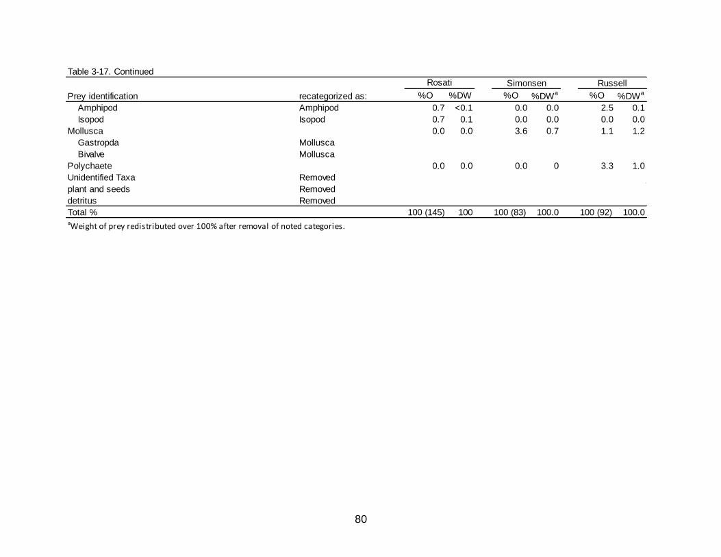
80
Table 3-17. Continued
recategorized as: %O %DW %O %DWa %O %DWa
Amphipod Amphipod 0.7 <0.1 0.0 0.0 2.5 0.1
Isopod Isopod 0.7 0.1 0.0 0.0 0.0 0.0
Mollusca 0.0 0.0 3.6 0.7 1.1 1.2
Gastropda Mollusca
Bivalve Mollusca
Polychaete 0.0 0.0 0.0 0 3.3 1.0
Unidentified Taxa Removed
plant and seeds Removed
detritus Removed
Total % 100 (145) 100 100 (83) 100.0 100 (92) 100.0aWeight of prey redistributed over 100% after removal of noted categories.
Prey identification
Rosati Simonsen Russell
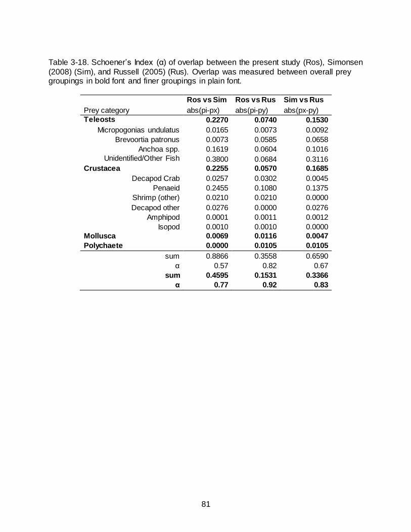
81
Table 3-18. Schoener’s Index (α) of overlap between the present study (Ros), Simonsen
(2008) (Sim), and Russell (2005) (Rus). Overlap was measured between overall prey groupings in bold font and finer groupings in plain font.
Prey category
Ros vs Sim Ros vs Rus Sim vs Rus
abs(pi-px) abs(pi-py) abs(px-py)
Teleosts 0.2270 0.0740 0.1530
Micropogonias undulatus 0.0165 0.0073 0.0092
Brevoortia patronus 0.0073 0.0585 0.0658
Anchoa spp. 0.1619 0.0604 0.1016
Unidentified/Other Fish 0.3800 0.0684 0.3116
Crustacea 0.2255 0.0570 0.1685
Decapod Crab 0.0257 0.0302 0.0045
Penaeid 0.2455 0.1080 0.1375
Shrimp (other) 0.0210 0.0210 0.0000
Decapod other 0.0276 0.0000 0.0276
Amphipod 0.0001 0.0011 0.0012
Isopod 0.0010 0.0010 0.0000
Mollusca 0.0069 0.0116 0.0047
Polychaete 0.0000 0.0105 0.0105
sum 0.8866 0.3558 0.6590
α 0.57 0.82 0.67
sum 0.4595 0.1531 0.3366
α 0.77 0.92 0.83
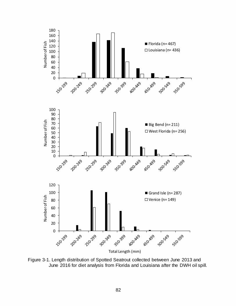
82
Figure 3-1. Length distribution of Spotted Seatrout collected between June 2013 and
June 2016 for diet analysis from Florida and Louisiana after the DWH oil spill.
020406080
100120140160180
Nu
mb
er o
f Fis
h Florida (n= 467)
Louisiana (n= 436)
0102030405060708090
100
Nu
mb
er o
f Fis
h
Big Bend (n= 211)
West Florida (n= 256)
0
20
40
60
80
100
120
Nu
mb
er o
f Fis
h
Total Length (mm)
Grand Isle (n= 287)
Venice (n= 149)
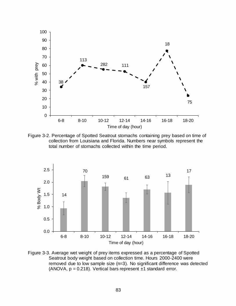
83
Figure 3-2. Percentage of Spotted Seatrout stomachs containing prey based on time of
collection from Louisiana and Florida. Numbers near symbols represent the
total number of stomachs collected within the time period.
Figure 3-3. Average wet weight of prey items expressed as a percentage of Spotted
Seatrout body weight based on collection time. Hours 2000-2400 were
removed due to low sample size (n=3). No significant difference was detected (ANOVA, p = 0.218). Vertical bars represent ±1 standard error.
38
113282 111
157
18
75
0
10
20
30
40
50
60
70
80
90
100
6-8 8-10 10-12 12-14 14-16 16-18 18-20
% w
ith pre
y
Time of day (hour)
14
70
159 61 63 1317
0.0
0.5
1.0
1.5
2.0
2.5
6-8 8-10 10-12 12-14 14-16 16-18 18-20
% B
ody
Wt
Time of day (hour)
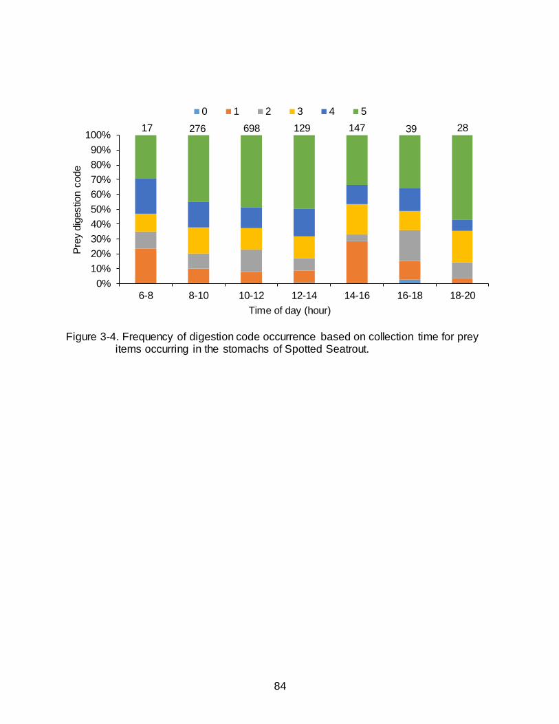
84
Figure 3-4. Frequency of digestion code occurrence based on collection time for prey
items occurring in the stomachs of Spotted Seatrout.
17 276 698 129 147 39 28
0%
10%
20%
30%
40%
50%
60%
70%
80%
90%
100%
6-8 8-10 10-12 12-14 14-16 16-18 18-20
Pre
y dig
estio
n c
ode
Time of day (hour)
0 1 2 3 4 5
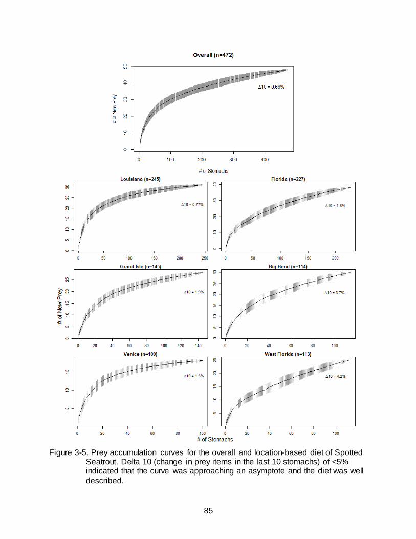
85
Figure 3-5. Prey accumulation curves for the overall and location-based diet of Spotted
Seatrout. Delta 10 (change in prey items in the last 10 stomachs) of <5% indicated that the curve was approaching an asymptote and the diet was well
described.
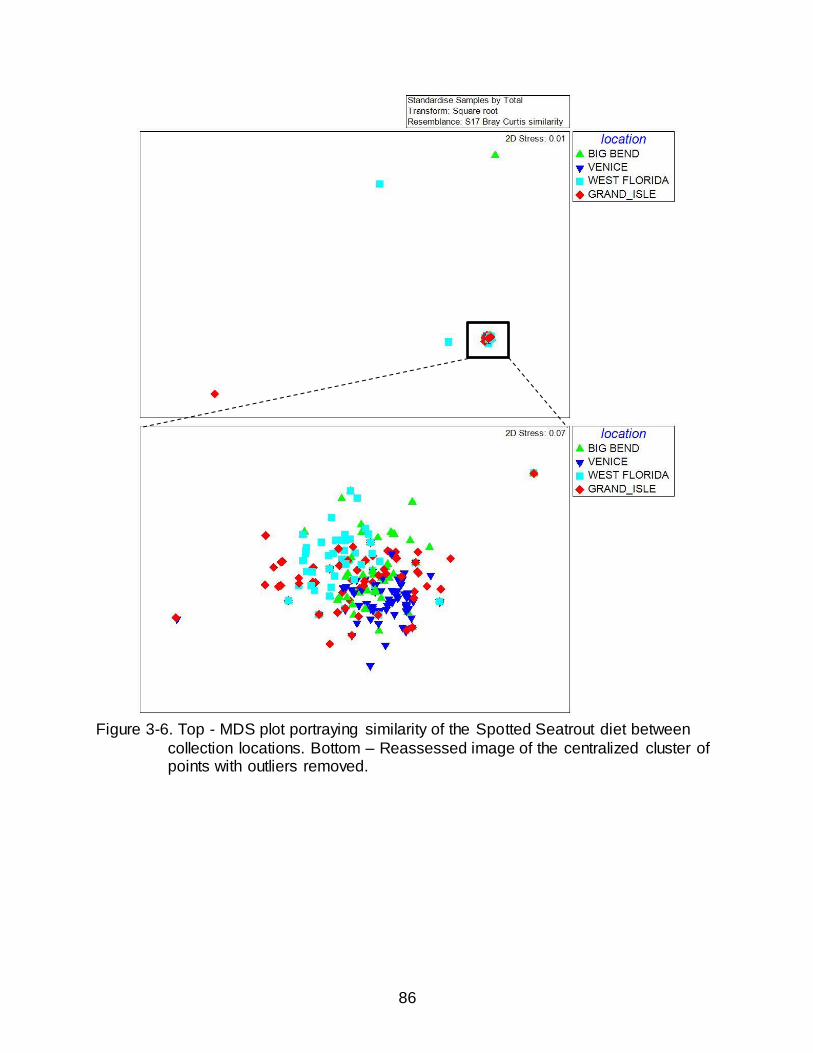
86
Figure 3-6. Top - MDS plot portraying similarity of the Spotted Seatrout diet between
collection locations. Bottom – Reassessed image of the centralized cluster of points with outliers removed.
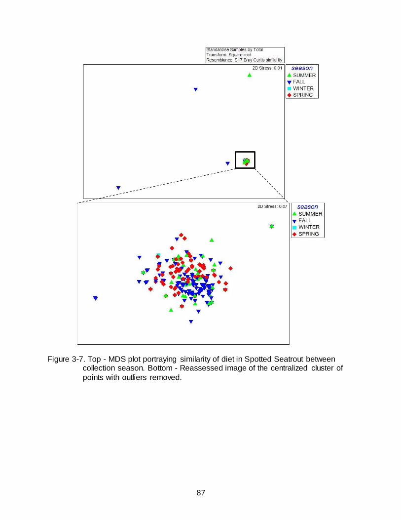
87
Figure 3-7. Top - MDS plot portraying similarity of diet in Spotted Seatrout between collection season. Bottom - Reassessed image of the centralized cluster of
points with outliers removed.
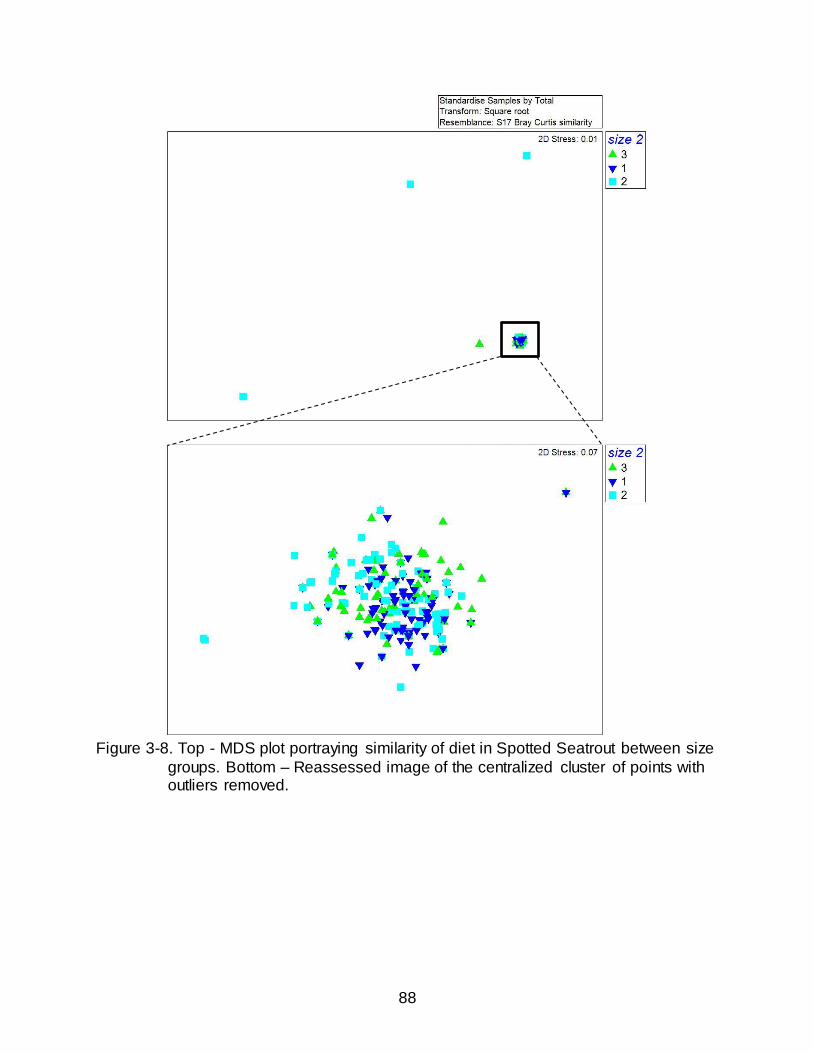
88
Figure 3-8. Top - MDS plot portraying similarity of diet in Spotted Seatrout between size
groups. Bottom – Reassessed image of the centralized cluster of points with outliers removed.
89
CHAPTER 4 DISCUSSION
Feeding Chronology
Most fishes exhibit predictive behaviors within a diel cycle that often lead to
changes in habitat, feeding intensity, and diet (Johnson and Dropkin 1993; Bowen
1996). Therefore, studies on the diets of fish must consider factors such as time of day,
light, water temperature, and the risk of predation which may influence feeding
behavior, and ultimately the diet, of fishes (Garvey and Chipps 2013). Based on mean
stomach content weight, digestion percentages of prey, and the frequency of empty
stomachs each as a function of time, Spotted Seatrout collected from FL and LA
appeared to have two diel feeding periods: a peak in feeding activity during the early to
mid-morning (0800-1000 h), and a smaller peak during the mid-afternoon (1600-1800
h). The sample size of Spotted Seatrout collected with stomach contents from 1600-
1800 h was small relative to the number of Spotted Seatrout with empty stomachs in the
surrounding time blocks, therefore, it is possible that only a small portion of Spotted
Seatrout feed at that time. Fishes of the same species typically display similar diel
behavioral patterns (Reebs 2003), however, deviations from this rhythm by specific
populations (Fraser et al. 1995; Valdimarsson et al. 2000), individuals at various
temperatures (Fraser et al. 1993), and by individuals of the same cohort experiencing
similar abiotic conditions (Sanchez-Vazquez et al. 1995; Alanara and Brannas 1997;
Metcalfe et al. 1998) have been documented. Diel cycles may also be altered in
response to changes in food availability or predator distribution (Bowen and Allanson
1982). Because of these potential variations, a comprehensive diet study must consider
diel activity when describing the diet of fishes.
90
Little has been previously published on the diel feeding activity of Spotted
Seatrout. Darnell (1958) identified peak stomach fullness at 1100 h followed by 8 h of
decreasing fullness in Spotted Seatrout collected in Lake Pontchartrain, LA. Darnell’s
results suggest peak feeding activity during the late-morning hours, and is relatively
consistent with the analysis of diel feeding activity of Spotted Seatrout collected in the
present study from southeastern Louisiana and the west coast of Florida. Darnell,
however, did not have stomach samples collected after 1700 h, whereas in the present
study an increase of minimally digested prey items accompanied by the decrease of
empty stomachs occurred between 1600-1800 h, suggesting a second period of late
afternoon feeding. Diet studies on other estuarine predators that have considered diel
activity have observed contributions of prey types that were previously thought to be of
little importance. Rock (2009) found mysids and other small bodied crustaceans
contributing to the nocturnal diet of Common Snook Centropomus undecimalis, which
were previously thought to only feed diurnally (McMichael et al. 1989). This oversight
may have led previous studies to over- or under-estimate the importance of prey
species occurring only during daylight hours in the diet of Common Snook. In the
present study, few Spotted Seatrout were collected during or after dusk, but fishermen
have reported Spotted Seatrout feeding at night near well-lit areas, such as dock and
bridge lights. However, such feeding behavior may only be indicative of the
opportunistic feeding behavior of Spotted Seatrout, due to the artificial attraction of
susceptible prey types to lights at night. This further suggests that Spotted Seatrout are
highly visual predators that rely on ambient conditions such as light availability and
water clarity to effectively forage (Minello and Zimmerman 1983). It is therefore
91
suggested that future studies on the diet of Spotted Seatrout incorporate a 24 h
sampling period to further confirm feeding periodicity, and potentially identify other
important prey that may not be present during daytime feeding.
Contemporary Diet of Spotted Seatrout
The contemporary diet of Spotted Seatrout analyzed in this study exhibited high
similarity and moderate overlap across locations spanning from Grand Isle, LA, to
Venice, LA, and from Horseshoe Beach, FL, to Charlotte Harbor, FL. Demersal fishes
(mainly Sciaenidae and Sparidae), pelagic fish (mainly Engraulidae and Clupeidae), and
decapod shrimp (mainly Penaeidae) were well represented in diet indices, and
appeared to be dominant prey items of Spotted Seatrout in southeastern Louisiana and
along the gulf coast of Florida. Pelagic fish made considerable contributions to the diet
of Spotted Seatrout in this study, however, their occurrence was strongly seasonal and
peaked during the fall. The contribution of pelagic fish by weight was similar between
summer and fall but the numerical abundance, particularly of Clupeiformes, doubled
from summer to fall. This is reflective of the increases in occurrence and numerical
abundance of smaller engraulids and subsequent decrease in numerical abundance of
larger clupeids, such as Gulf Menhaden, during the fall. The contribution of decapod
shrimp was also strongly seasonal, as occurrence, numerical abundance, and
reconstructed weight all peaked in the spring and declined through summer and fall.
Similar consistencies, both spatially and temporally, have been identified in other
recent post-spill diet studies of Spotted Seatrout in the northern Gulf of Mexico (Barnes
2014; Richards 2014). Richards (2014) identified fishes in the Engraulidae and
Sciaenidae families and penaeid shrimp as the most numerically abundant and
92
frequently occurring items in the diet of Spotted Seatrout in Apalachicola Bay, FL.
Similarly, engraulids, sciaenids, and penaeids were main contributors to the IRI
conducted by Barnes (2014) on Spotted Seatrout from Mississippi Sound, MS. The
seasonal comparison made by Barnes was limited to spring and summer because only
two fish contained prey in the fall and no fish were collected during the winter. Spotted
Seatrout collected by Barnes during the summer had seven prey categories while fish in
the spring contained only three prey categories (two of which were unidentified fish and
penaeid shrimp), which suggests a difference due to prey availability. Barnes (2014)
concluded little about the seasonal variation in diet due to small sample sizes during fall
and winter, therefore, the most recent seasonal diet observations of the Spotted
Seatrout are limited to Apalachicola Bay from 2010-2012 (Richards 2014). Richards
observed a large occurrence of penaeid shrimp during the spring, but also identified
natural annual variation in the occurrence of shrimp in the diet. Richards suggested
these seasonal changes appeared to be driven by differences in the seasonal
abundance and distribution of penaeid shrimp, as well as the natural variation in annual
abundance of other prey categories. The estuarine abundance of penaeid shrimp is
highly dependent on environmental conditions such as salinity and temperature
(Zimmerman and Minello 1984; Zein-Eldin and Renaud 1986; Jones et al. 2002). The
seasonal variation in the presence and absence of species in estuarine and coastal
habitats is also highly variable (McErlean et al 1973; Livingston 1976; Minello and
Zimmerman 1991; Jones et al. 2002; Akin et al. 2003). Given the generalist diet and
suggestive opportunistic feeding of Spotted Seatrout it is logical that they would feed on
readily available and seasonally abundant prey items.
93
The diet of Spotted Seatrout collected from Venice, LA, exhibited greater
variation when compared to other locations, especially West Florida, as indicated by
MDS, ANOSIM, and measures of overlap. Identified prey items were generally
consistent among locations, but the proportions of reconstructed weight in which they
contributed to the diet of Venice and West Florida were highly variable. These
differences could have been due to factors including sampling bias and variations in
habitat. The strong presence of engraulids and relative absence of penaeids in the diet
of Spotted Seatrout collected in Venice compared to West Florida could be due to
sampling bias. Of the 100 fish with stomach contents collected from Venice, 96 were
captured on a single sampling trip during the fall, a time when bay anchovies are most
abundant in the estuary (Robinette 1983). Further, only four fish with stomach contents
were collected from Venice during the spring and summer, seasons when penaeid
shrimp greatly contributed to the diet at other locations. An alternative explanation for
the detected difference could be attributed to variations in species assemblages due to
habitat type. Relatively similar IRI values across locations and coarser levels of prey
identification (i.e. fish versus shrimp and not family or species specific) suggest that for
Spotted Seatrout, a fish is a fish and a shrimp is a shrimp, but variations in available
species may exist between locations. Bays and estuaries of West Florida are rich with
seagrass beds, which are largely absent from the Mississippi River delta where Venice
is located (Comp and Seaman 1985; Peterson and Turner 1994). This is reflected in the
presence of seagrass associated families in the diet of West Florida Spotted Seatrout,
such as Sparidae (pinfish) and Haemulidae (pigfish), which were absent in the diet of
Spotted Seatrout from Venice.
94
Spotted Seatrout in the largest size group (size 3 > 350 mm TL) consumed more
demersal fish by %O, %N, and %RW than Spotted Seatrout in the smallest size group
(size 1: 150 – 299 mm TL). In general, larger Spotted Seatrout tended to consume
larger prey fishes (i.e. sciaenids, Lagodon rhomboides) than smaller Spotted Seatrout
which consumed greater amounts of smaller prey fish (Anchoa sp.). The greater
abundance of fish prey in the diet of large Spotted Seatrout is likely due to two reasons:
1) increased size and hence increased gape allows for consumption of larger prey; and
2) increased energetic demands. The allometric growth of fish is correlated to increases
in gape width and allows for the consumption of larger prey, which has been observed
in many predatory fish species (Scharf et al. 2000). Larger fish also have increased
energetic demands, often associated with increased fecundity, which can be met by
increasing consumption of calorie rich prey, such as fish (Persson 1988). Large adult
Spotted Seatrout have higher fecundity (Brown-Peterson et al. 2002) and subsequently
greater energetic demands than smaller adult Spotted Seatrout. Bioenergetically, an
increase in egg production requires an increase in energy intake to maintain a balanced
energy budget (Warren and Davis 1967). Therefore, to meet higher energy demands,
larger adult Spotted Seatrout must increase their consumption of prey items, such as
fish, that have high energy content. A greater amount of fish was also observed in the
diet of large adult Spotted Seatrout in previous studies conducted at Cedar Key and
Apalachicola, FL, and Lake Pontchartrain, LA (Moody 1950; Darnell 1958; Richards
2014).
Pre- and Post- DWH comparison of the Spotted Seatrout Diet
At its core, the diet of adult Spotted Seatrout before and after the DWH oil spill,
particularly in Barataria Bay, LA, has been comprised of primarily fish and shrimp. Any
95
observed differences between the pre- and post-spill studies compared here,
particularly those pertaining to the occurrence and dry weight of fish and crustaceans,
were difficult to attribute to the DWH oil spill. In pre-spill Barataria Bay, LA, Spotted
Seatrout collected between 2003-2007 exhibited high variability in the dietary
contributions of fish and shrimp (Russell 2005; Simonsen 2008). Russell (2005)
observed approximately 15% more fish and 13% less penaeid shrimp by DW compared
to Simonsen (2008). Comparatively, the present post-spill study, based on Spotted
Seatrout collected in 2013-2016, observed relatively small differences in the dietary
contribution by DW of fish (+7%) and penaeid shrimp (-10%) when compared to
Russell, but relatively large differences in fish (+23%) and shrimp (-23%) compared to
Simonsen. This resulted in the diets of the present study and the pre-spill study by
Russell being more similar than the comparison between the pre-spill studies of Russell
and Simonsen. Therefore, the observed differences in pre-and post-spill diet of Spotted
Seatrout from Barataria Bay, LA, could possibly be attributed to natural annual variation
in their diet based on the availability of fish or shrimp, as opposed to direct food web
changes following the DWH oil spill. Furthermore, no large shifts or variations in prey
resource utilization nor increases or decreases in the consumption of lower or higher
trophic level prey types, as seen in other species (Norberg 2015, Tarnecki and
Patterson 2015), were observed in the post-spill Spotted Seatrout diet.
Comparisons of dietary overlap, or how much of the diet was shared between
studies, can also help identify changes in diet or feeding behavior. Despite the observed
variations in proportional usage among prey resources between the pre-spill and
present post-spill study, dietary overlap was moderate to high and suggests that
96
Spotted Seatrout have had little relative change in their diet between 2003-2007 (before
the DWH oil spill) and 2013-2016 (3 years after the DWH oil spill). Diet overlap was also
greater between the present study and the pre-spill study of Russell (2005), than the
overlap between the two pre-spill studies of Russell (2005) and Simonsen (2008),
further reiterating the large variation in prey resource utilization among studies.
Additionally, while not directly compared here, the dietary breadth observed in Spotted
Seatrout collected in Barataria Bay, LA, during the present study (J’=0.69) was similar to
Russell’s pre-spill study (J’=0.73). This suggests that Spotted Seatrout have maintained
a broad generalist diet both before and after the DWH oil spill, which is consistent with
other pre-spill descriptions. The large amount of different fishes identified in the diet of
Spotted Seatrout suggests they are primarily piscivorous but will readily feed on other
available prey types. Further, the wide dietary breadth suggests high plasticity,
increasing the resiliency of Spotted Seatrout if a prey resource is reduced or eliminated.
Contrarily, predators with a narrow diet limited to few prey types, could be greatly
affected in the event a prey resource became limited. Carnivorous fishes, such as the
Spotted Seatrout, have been deemed highly important to the estuarine food web and
models indicate that, in a trophic ecology sense, they are relatively insensitive to oil, and
in turn, help stabilize ecosystem resiliency (McCann et al. 2017). This is likely due in
part to the observed broad diet of Spotted Seatrout and their ability to prey upon
multiple taxa and maintain their ecological role within the estuary and nearshore waters.
The resolution of prey identification in the present study was generally higher
than in previous diet studies of Spotted Seatrout. This was made clear in the large
number of identified fishes in the present study relative to the large amount of
97
unidentified fish observed in the pre-spill studies (Russell 2005; Simonsen 2008). The
low resolution in prey identification among the pre-spill studies of Russell and Simonsen
was an issue when making pre- and post-spill dietary comparisons, especially when
questions of diet alterations were considered. Decisions regarding whether Spotted
Seatrout have increased diet diversity after the DWH oil spill were difficult to make when
the resolution of prey identification among studies was so marked. It was possible that
prey diversity in the pre-spill diet was lost by being pooled into ‘unidentified’ categories,
or contrarily, those prey types were never encountered. However, many of the
additional prey items identified in the present study have been previously observed in
the diet of Spotted Seatrout by researchers prior to the DWH oil spill (Gunter 1945;
Moody 1950; Darnell 1958, Overstreet 1982), suggesting the diet in recent pre-spill
studies was either not well described or prey were unidentified. Higher taxonomic
resolution would increase the likelihood of identifying changes in the prey base of
predatory fishes. Many of the prey resource categories identified in the present study
needed to be reclassified to higher taxonomic levels to make the comparison between
the pre-and post-spill diet of Spotted Seatrout, and thus reduced our ability to identify
potential biologically significant differences in the consumption of specific prey. Because
of this limitation, only very large differences in the diet of Spotted Seatrout would have
been identified.
The increased resolution of prey identification in the present study was likely due
to the use of otoliths to identify prey fishes and sampling during peak feeding times.
Many species of fish have uniquely shaped otoliths which can aid in identification, often
to the family and genus taxonomic level, as well as aid in the reconstruction of whole
98
prey weight (Harkonen 1986; Baremore and Bethea 2010). It is unclear whether
previous Spotted Seatrout diet studies used otoliths as an aid in prey fish identification,
but their increased percentages of unidentified fish suggests not. Additionally, targeting
Spotted Seatrout during known feeding times decreases the elapsed time since feeding,
which results in collecting stomachs with recently consumed prey, enhancing the prey
identification process and increasing taxonomic resolution.
The quality of pre-spill data was a factor in my ability to draw comparison and
make more decisive conclusions regarding potential impacts of the DWH oil spill on the
diet of Spotted Seatrout. It was difficult to say if the diet of Spotted Seatrout was well
described by previous studies due to a lack of prey accumulation curves. Additionally,
there is an inherent bias in using partial and digested prey weights (Russell 2005;
Simonsen 2008) as opposed to the reconstructed weight of a prey item (present study),
because of the variation in time since prey consumption and therefore how much
digestion has occurred (Bromley 1994; Bowen 1996; Garvey and Chipps 2013). For
example, a consumed anchovy weighing 3 g will weigh far less 3 h after consumption
when it is 50% digested as opposed to 1 h after consumption when only 10% digested.
In contrast, if a regression equation is used to reconstruct the whole weight of the
anchovy when it was consumed, then the original weight of the anchovy stays the same
regardless of digestion state. Typically, diet studies do not utilize reconstructed weights
of prey items as it can be very time consuming to build length-weight regressions,
however, it is important to reconstruct the diet fully when considering biological
implications. Using partial prey weights is likely to lead to the underestimation of prey
utilization, and when used with models dependent on these data, will underestimate
99
meal size and energy intake (e.g. there are more calories in 3 g of anchovy than 1 g of
anchovy). Further, the digestion rate of different prey items varies, with shrimp and crab
digesting slower than fish due to their exoskeleton (Bromley 1994). This is another
reason to sample throughout the diel cycle and use reconstructed weights or risk
underestimating or completely missing important prey resources (Bromley 1994; Rock
2009). Variation in digestion and capture times could therefore explain some of the
observed differences in the DW contribution between fish and shrimp among the three
comparative diet studies from Barataria Bay, LA.
Indirect effects of ecosystem disturbances, such as the DWH oil spill, have a
proven history of disrupting trophic interactions and altering the predator-prey dynamics
within a system (Alonso et al. 2002; Link and Garrison 2002; Peterson et al. 2003;
Tarnecki and Patterson 2015). The present study observed a similar post-spill diet of
Spotted Seatrout across most of its range in the north-eastern Gulf of Mexico, and prey
resource categories were consistent with other post-spill diet studies of Spotted
Seatrout (Barnes 2011, Richards 2014). No large shift in prey resource categories was
detected, suggesting little change in the overall diet between oiled and non-oiled
regions and pre- and post-spill diets. The dissimilarities that existed between sites, such
as those between Venice, LA, and West Florida, may have been due to differences in
species assemblages and the natural variation in annual prey abundance opposed to
true dietary changes, which could have led to trophic level shifts such as those identified
in other post-spill diet studies (Norberg 2015; Tarnecki and Patterson 2015). Without
having site-specific density and abundance data for individual prey species, it was
difficult to disregard the natural annual variation in diet and prey abundance as a
100
potential factor. The pre-and post-spill comparison of the Spotted Seatrout diet in
Barataria Bay determined that there was high dietary overlap and similar prey
categories utilized, but moderate differences in the proportions by dry weight existed.
The variation in proportional usage may have been due to the bias in using digested
prey weights as opposed to reconstructed whole prey weight to assess diet. However,
this bias is unlikely to account for the overall natural variation in prey resource utilization
observed among pre-spill diets. Furthermore, the comparison between pre-spill studies
was less similar than comparison between pre- and post-spill studies, suggestive of
high annual variation in resource utilization, and the variation in the post-spill diet did not
appear greater than what occurred in Barataria Bay, LA, prior to the DWH oil spill.
Multiple techniques are available for diet analysis, and replication of results and
the ability to draw future comparisons, while limiting bias, should be kept in mind when
deciding on an appropriate study design. In light of the DWH oil spill, it has been made
clear that increasing monitoring programs to improve available baseline data to assess
before and after conditions is imperative. This study therefore also provides a source of
highly detailed baseline dietary data for the Spotted Seatrout across locations in the
northern Gulf of Mexico, useful in the event of another potential large-scale ecosystem
disturbance.

101
APPENDIX WET AND DRY WEIGHTS
Wet and dry weight values of prey categories identified in the post-DWH oil spill diet of Spotted Seatrout. Values are presented for diets based on location, season, and size.
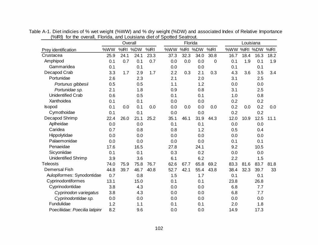
102
Table A-1. Diet indicies of % wet weight (%WW) and % dry weight (%DW) and associated Index of Relative Importance (%IRI) for the overall, Florida, and Louisiana diet of Spotted Seatrout.
%WW %IRI %DW %IRI %WW %IRI %DW %IRI %WW %IRI %DW %IRI
25.9 24.1 24.1 23.3 37.3 32.3 34.0 30.8 16.7 18.4 16.3 18.2
0.1 0.7 0.1 0.7 0.0 0.0 0.0 0 0.1 1.9 0.1 1.9
0.1 0.1 0.0 0.0 0.1 0.1
3.3 1.7 2.9 1.7 2.2 0.3 2.1 0.3 4.3 3.6 3.5 3.4
2.6 2.3 2.1 2.0 3.1 2.5
Portunus gibbesii 0.5 0.5 1.1 1.2 0.0 0.0
Portunidae sp. 2.1 1.8 0.9 0.8 3.1 2.5
0.6 0.5 0.1 0.1 1.0 0.8
0.1 0.1 0.0 0.0 0.2 0.2
0.1 0.0 0.1 0.0 0.0 0.0 0.0 0.0 0.2 0.0 0.2 0.0
0.1 0.1 0.0 0.0 0.2 0.2
22.4 26.0 21.1 25.2 35.1 46.1 31.9 44.3 12.0 10.9 12.5 11.1
0.0 0.0 0.1 0.1 0.0 0.0
0.7 0.8 0.8 1.2 0.5 0.4
0.0 0.0 0.0 0.0 0.0 0.0
0.0 0.0 0.0 0.0 0.1 0.1
17.6 16.5 27.8 24.1 9.2 10.5
0.1 0.1 0.3 0.2 0.0 0.0
3.9 3.6 6.1 6.2 2.2 1.5
74.0 75.9 75.8 76.7 62.6 67.7 65.8 69.2 83.3 81.6 83.7 81.8
44.8 39.7 46.7 40.8 52.7 42.1 55.4 43.8 38.4 32.3 39.7 33
0.7 0.8 1.5 1.7 0.1 0.1
13.1 15.0 0.1 0.1 23.8 26.8
3.8 4.3 0.0 0.0 6.8 7.7
Cyprinodon variegatus 3.8 4.3 0.0 0.0 6.8 7.7
Cyprinodontidae sp. 0.0 0.0 0.0 0.0 0.0 0.0
1.2 1.1 0.1 0.1 2.0 1.8
8.2 9.6 0.0 0.0 14.9 17.3
Aulopiformes: Synodontidae
Cyprinodontiformes
Cyprinodontidae
Fundulidae
Poeciliidae: Poecilia latipinna
Demersal Fish
Isopod
Cymothoidae
Decapod Shrimp
Aplheidae
Caridea
Hippolytidae
Palaemonidae
Penaeidae
Sicyoniidae
Unidentified Shrimp
Teleosts
Xanthoidea
Crustacea
Prey identification
LouisianaFloridaOverall
Amphipod
Gammaridea
Decapod Crab
Portunidae
Unidentified Crab
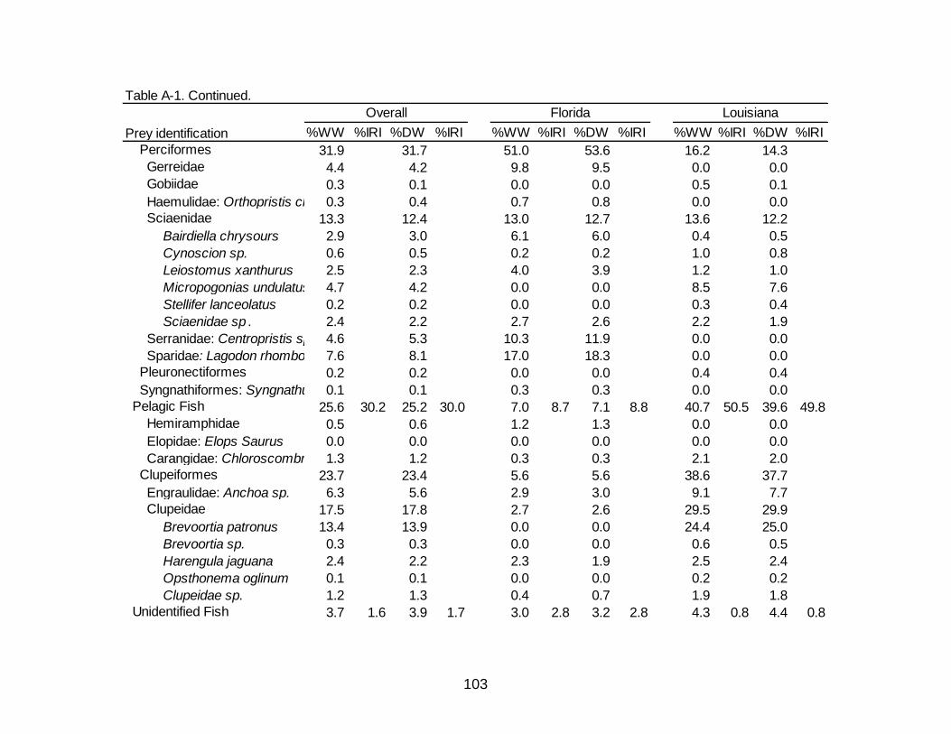
103
%WW %IRI %DW %IRI %WW %IRI %DW %IRI %WW %IRI %DW %IRI
31.9 31.7 51.0 53.6 16.2 14.3
4.4 4.2 9.8 9.5 0.0 0.0
0.3 0.1 0.0 0.0 0.5 0.1
0.3 0.4 0.7 0.8 0.0 0.0
13.3 12.4 13.0 12.7 13.6 12.2
Bairdiella chrysours 2.9 3.0 6.1 6.0 0.4 0.5
Cynoscion sp. 0.6 0.5 0.2 0.2 1.0 0.8
Leiostomus xanthurus 2.5 2.3 4.0 3.9 1.2 1.0
Micropogonias undulatus 4.7 4.2 0.0 0.0 8.5 7.6
Stellifer lanceolatus 0.2 0.2 0.0 0.0 0.3 0.4
Sciaenidae sp . 2.4 2.2 2.7 2.6 2.2 1.9
4.6 5.3 10.3 11.9 0.0 0.0
7.6 8.1 17.0 18.3 0.0 0.0
0.2 0.2 0.0 0.0 0.4 0.4
0.1 0.1 0.3 0.3 0.0 0.0
25.6 30.2 25.2 30.0 7.0 8.7 7.1 8.8 40.7 50.5 39.6 49.8
0.5 0.6 1.2 1.3 0.0 0.0
0.0 0.0 0.0 0.0 0.0 0.0
1.3 1.2 0.3 0.3 2.1 2.0
23.7 23.4 5.6 5.6 38.6 37.7
6.3 5.6 2.9 3.0 9.1 7.7
17.5 17.8 2.7 2.6 29.5 29.9
Brevoortia patronus 13.4 13.9 0.0 0.0 24.4 25.0
Brevoortia sp. 0.3 0.3 0.0 0.0 0.6 0.5
Harengula jaguana 2.4 2.2 2.3 1.9 2.5 2.4
Opsthonema oglinum 0.1 0.1 0.0 0.0 0.2 0.2
Clupeidae sp. 1.2 1.3 0.4 0.7 1.9 1.8
3.7 1.6 3.9 1.7 3.0 2.8 3.2 2.8 4.3 0.8 4.4 0.8
Engraulidae: Anchoa sp.
Clupeidae
Unidentified Fish
Clupeiformes
Gobiidae
Haemulidae: Orthopristis chrysoptera
Sciaenidae
Serranidae: Centropristis sp.
Sparidae: Lagodon rhomboides
Pleuronectiformes
Syngnathiformes: Syngnathus floridae
Pelagic Fish
Hemiramphidae
Elopidae: Elops Saurus
Carangidae: Chloroscombrus chrysurus
Perciformes
Gerreidae
Prey identification
Overall Florida Louisiana
Table A-1. Continued.
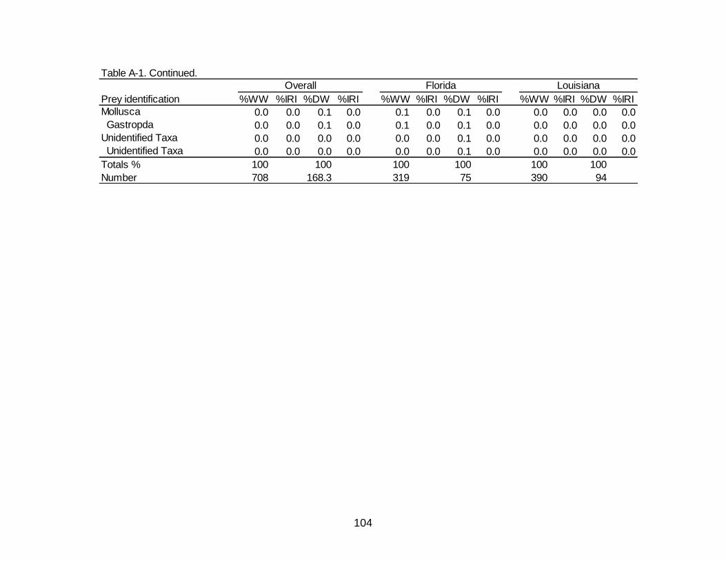
104
%WW %IRI %DW %IRI %WW %IRI %DW %IRI %WW %IRI %DW %IRI
0.0 0.0 0.1 0.0 0.1 0.0 0.1 0.0 0.0 0.0 0.0 0.0
0.0 0.0 0.1 0.0 0.1 0.0 0.1 0.0 0.0 0.0 0.0 0.0
0.0 0.0 0.0 0.0 0.0 0.0 0.1 0.0 0.0 0.0 0.0 0.0
0.0 0.0 0.0 0.0 0.0 0.0 0.1 0.0 0.0 0.0 0.0 0.0
Totals % 100 100 100 100 100 100
Number 708 168.3 319 75 390 94
Mollusca
Gastropda
Unidentified Taxa
Unidentified Taxa
Prey identification
Overall Florida Louisiana
Table A-1. Continued.
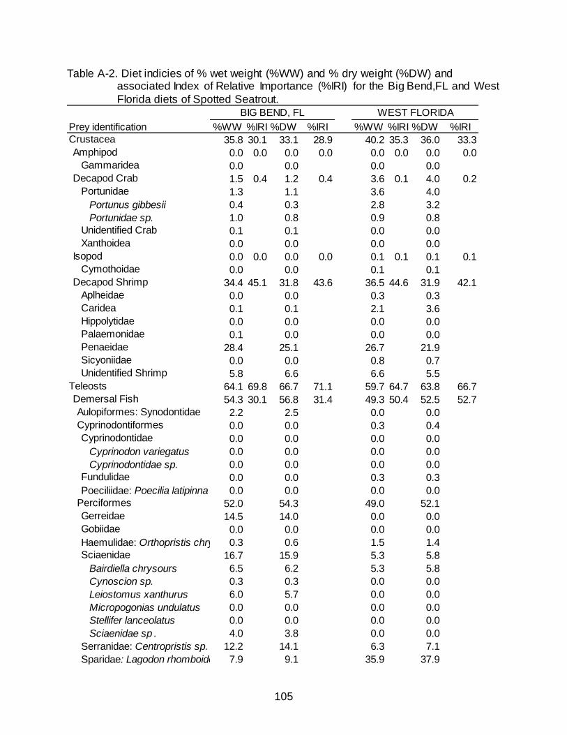
105
Table A-2. Diet indicies of % wet weight (%WW) and % dry weight (%DW) and associated Index of Relative Importance (%IRI) for the Big Bend,FL and West
Florida diets of Spotted Seatrout.
%WW %IRI %DW %IRI %WW %IRI %DW %IRI
35.8 30.1 33.1 28.9 40.2 35.3 36.0 33.3
0.0 0.0 0.0 0.0 0.0 0.0 0.0 0.0
0.0 0.0 0.0 0.0
1.5 0.4 1.2 0.4 3.6 0.1 4.0 0.2
1.3 1.1 3.6 4.0
Portunus gibbesii 0.4 0.3 2.8 3.2
Portunidae sp. 1.0 0.8 0.9 0.8
0.1 0.1 0.0 0.0
0.0 0.0 0.0 0.0
0.0 0.0 0.0 0.0 0.1 0.1 0.1 0.1
0.0 0.0 0.1 0.1
34.4 45.1 31.8 43.6 36.5 44.6 31.9 42.1
0.0 0.0 0.3 0.3
0.1 0.1 2.1 3.6
0.0 0.0 0.0 0.0
0.1 0.0 0.0 0.0
28.4 25.1 26.7 21.9
0.0 0.0 0.8 0.7
5.8 6.6 6.6 5.5
64.1 69.8 66.7 71.1 59.7 64.7 63.8 66.7
54.3 30.1 56.8 31.4 49.3 50.4 52.5 52.7
2.2 2.5 0.0 0.0
0.0 0.0 0.3 0.4
0.0 0.0 0.0 0.0
Cyprinodon variegatus 0.0 0.0 0.0 0.0
Cyprinodontidae sp. 0.0 0.0 0.0 0.0
0.0 0.0 0.3 0.3
0.0 0.0 0.0 0.0
52.0 54.3 49.0 52.1
14.5 14.0 0.0 0.0
0.0 0.0 0.0 0.0
0.3 0.6 1.5 1.4
16.7 15.9 5.3 5.8
Bairdiella chrysours 6.5 6.2 5.3 5.8
Cynoscion sp. 0.3 0.3 0.0 0.0
Leiostomus xanthurus 6.0 5.7 0.0 0.0
Micropogonias undulatus 0.0 0.0 0.0 0.0
Stellifer lanceolatus 0.0 0.0 0.0 0.0
Sciaenidae sp . 4.0 3.8 0.0 0.0
12.2 14.1 6.3 7.1
7.9 9.1 35.9 37.9
WEST FLORIDABIG BEND, FL
Serranidae: Centropristis sp.
Sparidae: Lagodon rhomboides
Sciaenidae
Teleosts
Demersal Fish
Aulopiformes: Synodontidae
Cyprinodontiformes
Cyprinodontidae
Fundulidae
Poeciliidae: Poecilia latipinna
Perciformes
Gerreidae
Gobiidae
Haemulidae: Orthopristis chrysoptera
Amphipod
Gammaridea
Decapod Crab
Portunidae
Unidentified Shrimp
Unidentified Crab
Xanthoidea
Isopod
Cymothoidae
Decapod Shrimp
Aplheidae
Caridea
Hippolytidae
Palaemonidae
Penaeidae
Sicyoniidae
Prey identification
Crustacea
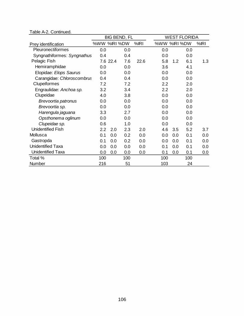
106
%WW %IRI %DW %IRI %WW %IRI %DW %IRI
0.0 0.0 0.0 0.0
0.4 0.4 0.0 0.0
7.6 22.4 7.6 22.6 5.8 1.2 6.1 1.3
0.0 0.0 3.6 4.1
0.0 0.0 0.0 0.0
0.4 0.4 0.0 0.0
7.2 7.2 2.2 2.0
3.2 3.4 2.2 2.0
4.0 3.8 0.0 0.0
Brevoortia patronus 0.0 0.0 0.0 0.0
Brevoortia sp. 0.0 0.0 0.0 0.0
Harengula jaguana 3.3 2.7 0.0 0.0
Opsthonema oglinum 0.0 0.0 0.0 0.0
Clupeidae sp. 0.6 1.0 0.0 0.0
2.2 2.0 2.3 2.0 4.6 3.5 5.2 3.7
0.1 0.0 0.2 0.0 0.0 0.0 0.1 0.0
0.1 0.0 0.2 0.0 0.0 0.0 0.1 0.0
0.0 0.0 0.0 0.0 0.1 0.0 0.1 0.0
0.0 0.0 0.0 0.0 0.1 0.0 0.1 0.0
100 100 100 100
216 51 103 24
Unidentified Taxa
Unidentified Taxa
Total %
Number
BIG BEND, FL WEST FLORIDA
Clupeiformes
Engraulidae: Anchoa sp.
Clupeidae
Unidentified Fish
Mollusca
Gastropda
Pleuronectiformes
Syngnathiformes: Syngnathus floridae
Pelagic Fish
Hemiramphidae
Elopidae: Elops Saurus
Carangidae: Chloroscombrus chrysurus
Table A-2. Continued.
Prey identification

107
Table A-3. Diet indicies of % wet weight (%WW) and % dry weight (%DW) and associated Index of Relative Importance (%IRI) for the Grand Isle, LA and
Venice diets of Spotted Seatrout.
%WW %IRI %DW %IRI %WW %IRI %DW %IRI
20.8 23.2 20.9 23.2 64.0 13.5 7.0 12.8
0.0 0.0 0.0 0.0 34.0 3.9 0.3 3.9
0.0 0.0 34.0 0.3
4.1 1.6 3.6 1.6 30.0 1.5 3.4 3.2
3.1 2.8 16.0 2.1
Portunus gibbesii 0.0 0.0 0.0 0.0
Portunidae sp. 3.1 2.8 16.0 2.1
0.7 0.5 17.0 1.3
0.3 0.3 0.0 0.0
0.1 0.0 0.1 0.0 5.0 0.1 0.4 0.0
0.1 0.1 5.0 0.4
16.6 23.6 17.2 23.7 18.0 1.0 2.9 1.0
0.0 0.0 0.0 0.0
0.6 0.5 4.0 0.3
0.0 0.0 0.0 0.0
0.0 0.0 1.0 0.2
13.3 15.1 3.0 1.3
0.0 0.0 0.0 0.0
2.6 1.6 12.0 1.1
79.2 76.8 79.1 76.8 92.0 86.5 93.0 87.2
52.5 67.5 54.1 67.9 20.0 2.5 10.5 2.3
0.2 0.2 0.0 0.0
33.3 37.3 3.0 5.6
10.5 11.5 0.0 0.0
Cyprinodon variegatus 10.5 11.5 0.0 0.0
Cyprinodontidae sp. 0.0 0.0 0.0 0.0
0.0 0.0 3.0 5.6
22.8 25.8 0.0 0.0
21.7 18.9 18.0 5.0
0.0 0.0 0.0 0.0
0.6 0.1 1.0 0.2
0.0 0.0 0.0 0.0
17.8 15.9 17.0 4.8
Bairdiella chrysours 0.6 0.8 0.0 0.0
Cynoscion sp. 1.5 1.2 1.0 0.0
Leiostomus xanthurus 1.8 1.6 2.0 0.0
Micropogonias undulatus 13.0 11.3 0.0 0.0
Stellifer lanceolatus 0.5 0.6 0.0 0.0
Sciaenidae sp . 0.5 0.4 14.0 4.8
0.0 0.0 0.0 0.0
0.0 0.0 0.0 0.0Sparidae: Lagodon rhomboides
Perciformes
Gerreidae
Gobiidae
Haemulidae: Orthopristis chrysoptera
Sciaenidae
Serranidae: Centropristis sp.
Poeciliidae: Poecilia latipinna
Hippolytidae
Palaemonidae
Penaeidae
Sicyoniidae
Unidentified Shrimp
Teleosts
Demersal Fish
Aulopiformes: Synodontidae
Cyprinodontiformes
Cyprinodontidae
Fundulidae
Caridea
Crustacea
Amphipod
Gammaridea
Decapod Crab
Portunidae
Unidentified Crab
Xanthoidea
Isopod
Cymothoidae
Decapod Shrimp
Aplheidae
Prey identification
GRAND ISLE, LA VENICE, LA
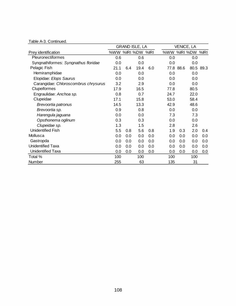
108
%WW %IRI %DW %IRI %WW %IRI %DW %IRI
0.6 0.6 0.0 0.0
0.0 0.0 0.0 0.0
21.1 6.4 19.4 6.0 77.8 88.6 80.5 89.3
0.0 0.0 0.0 0.0
0.0 0.0 0.0 0.0
3.2 2.9 0.0 0.0
17.9 16.5 77.8 80.5
0.8 0.7 24.7 22.0
17.1 15.8 53.0 58.4
Brevoortia patronus 14.5 13.3 42.9 48.6
Brevoortia sp. 0.9 0.8 0.0 0.0
Harengula jaguana 0.0 0.0 7.3 7.3
Opsthonema oglinum 0.3 0.3 0.0 0.0
Clupeidae sp. 1.3 1.5 2.8 2.6
5.5 0.8 5.6 0.8 1.9 0.3 2.0 0.4
0.0 0.0 0.0 0.0 0.0 0.0 0.0 0.0
0.0 0.0 0.0 0.0 0.0 0.0 0.0 0.0
0.0 0.0 0.0 0.0 0.0 0.0 0.0 0.0
0.0 0.0 0.0 0.0 0.0 0.0 0.0 0.0
100 100 100 100
255 63 135 31
Unidentified Taxa
Total %
Number
Engraulidae: Anchoa sp.
Clupeidae
Unidentified Fish
Mollusca
Gastropda
Unidentified Taxa
Clupeiformes
Table A-3. Continued.
Prey identification
GRAND ISLE, LA
Syngnathiformes: Syngnathus floridae
Pelagic Fish
Hemiramphidae
Elopidae: Elops Saurus
Carangidae: Chloroscombrus chrysurus
VENICE, LA
Pleuronectiformes
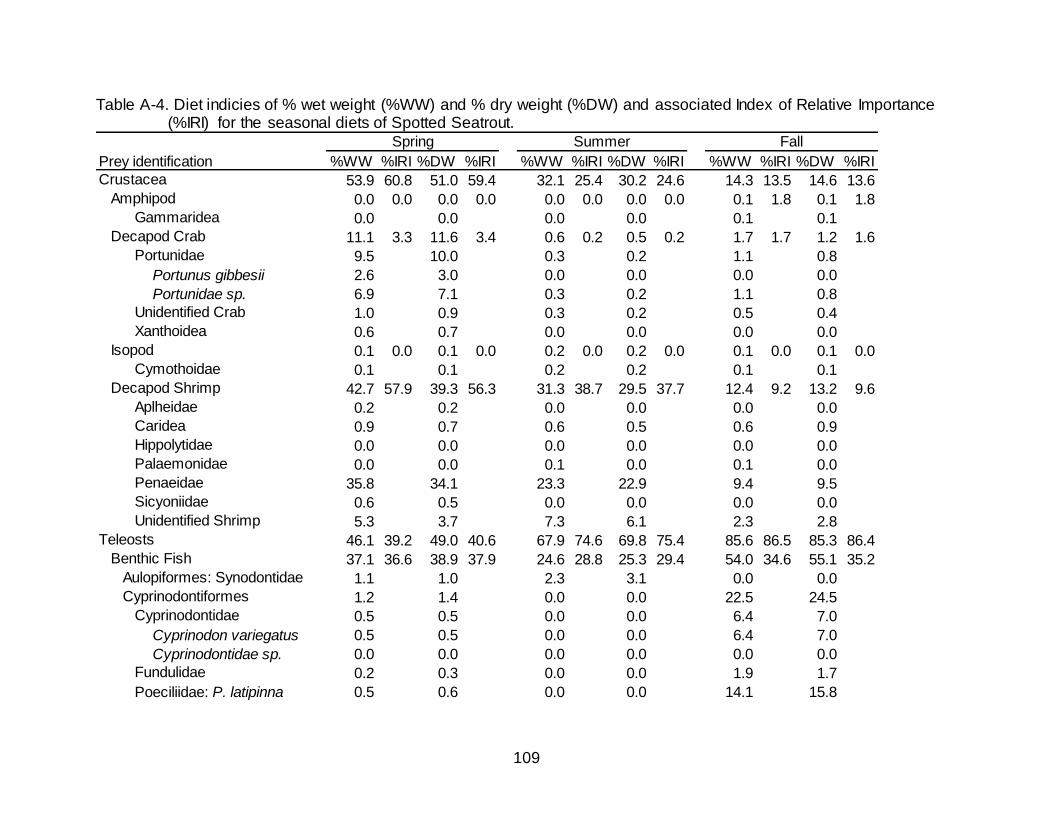
109
Table A-4. Diet indicies of % wet weight (%WW) and % dry weight (%DW) and associated Index of Relative Importance (%IRI) for the seasonal diets of Spotted Seatrout.
%WW %IRI %DW %IRI %WW %IRI %DW %IRI %WW %IRI %DW %IRI
53.9 60.8 51.0 59.4 32.1 25.4 30.2 24.6 14.3 13.5 14.6 13.6
0.0 0.0 0.0 0.0 0.0 0.0 0.0 0.0 0.1 1.8 0.1 1.8
0.0 0.0 0.0 0.0 0.1 0.1
11.1 3.3 11.6 3.4 0.6 0.2 0.5 0.2 1.7 1.7 1.2 1.6
9.5 10.0 0.3 0.2 1.1 0.8
Portunus gibbesii 2.6 3.0 0.0 0.0 0.0 0.0
Portunidae sp. 6.9 7.1 0.3 0.2 1.1 0.8
1.0 0.9 0.3 0.2 0.5 0.4
0.6 0.7 0.0 0.0 0.0 0.0
0.1 0.0 0.1 0.0 0.2 0.0 0.2 0.0 0.1 0.0 0.1 0.0
0.1 0.1 0.2 0.2 0.1 0.1
42.7 57.9 39.3 56.3 31.3 38.7 29.5 37.7 12.4 9.2 13.2 9.6
0.2 0.2 0.0 0.0 0.0 0.0
0.9 0.7 0.6 0.5 0.6 0.9
0.0 0.0 0.0 0.0 0.0 0.0
0.0 0.0 0.1 0.0 0.1 0.0
35.8 34.1 23.3 22.9 9.4 9.5
0.6 0.5 0.0 0.0 0.0 0.0
5.3 3.7 7.3 6.1 2.3 2.8
46.1 39.2 49.0 40.6 67.9 74.6 69.8 75.4 85.6 86.5 85.3 86.4
37.1 36.6 38.9 37.9 24.6 28.8 25.3 29.4 54.0 34.6 55.1 35.2
1.1 1.0 2.3 3.1 0.0 0.0
1.2 1.4 0.0 0.0 22.5 24.5
0.5 0.5 0.0 0.0 6.4 7.0
Cyprinodon variegatus 0.5 0.5 0.0 0.0 6.4 7.0
Cyprinodontidae sp. 0.0 0.0 0.0 0.0 0.0 0.0
0.2 0.3 0.0 0.0 1.9 1.7
0.5 0.6 0.0 0.0 14.1 15.8
Palaemonidae
Penaeidae
Sicyoniidae
Unidentified Shrimp
Teleosts
Benthic Fish
Aulopiformes: Synodontidae
Cyprinodontiformes
Cyprinodontidae
Fundulidae
Poeciliidae: P. latipinna
Hippolytidae
Amphipod
Gammaridea
Decapod Crab
Portunidae
Unidentified Crab
Xanthoidea
Isopod
Cymothoidae
Decapod Shrimp
Aplheidae
Caridea
Fall
Crustacea
Prey identification
Spring Summer
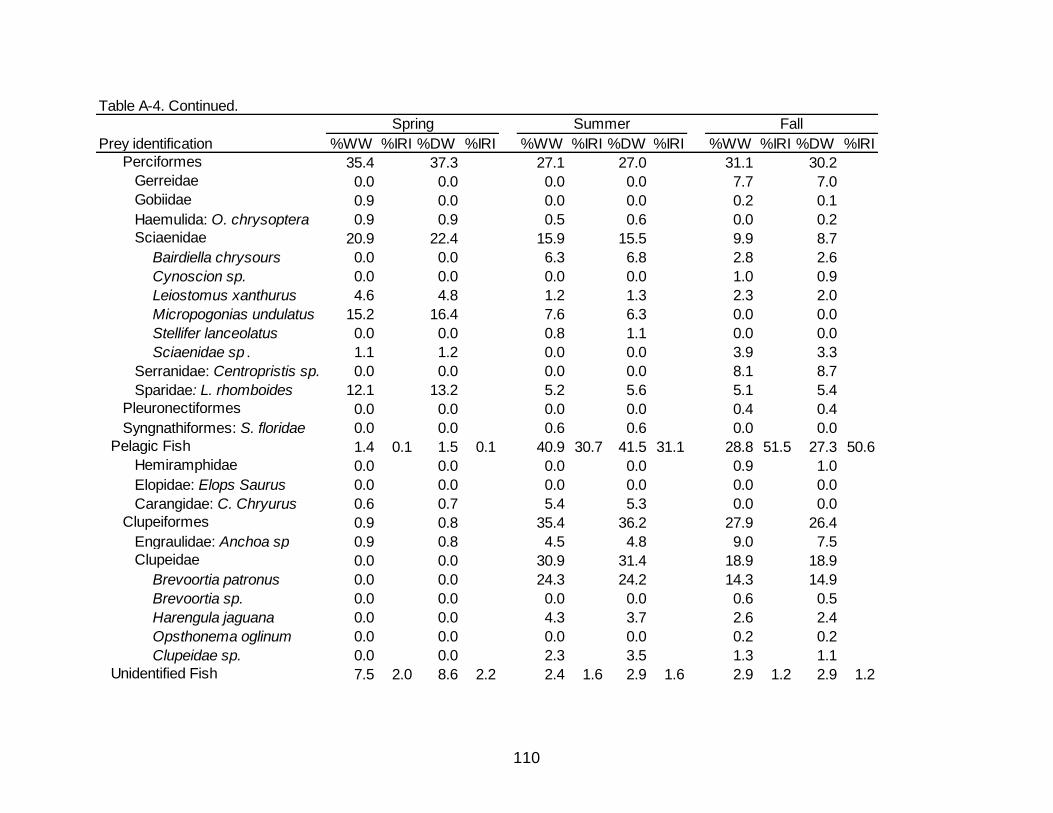
110
%WW %IRI %DW %IRI %WW %IRI %DW %IRI %WW %IRI %DW %IRI
35.4 37.3 27.1 27.0 31.1 30.2
0.0 0.0 0.0 0.0 7.7 7.0
0.9 0.0 0.0 0.0 0.2 0.1
0.9 0.9 0.5 0.6 0.0 0.2
20.9 22.4 15.9 15.5 9.9 8.7
Bairdiella chrysours 0.0 0.0 6.3 6.8 2.8 2.6
Cynoscion sp. 0.0 0.0 0.0 0.0 1.0 0.9
Leiostomus xanthurus 4.6 4.8 1.2 1.3 2.3 2.0
Micropogonias undulatus 15.2 16.4 7.6 6.3 0.0 0.0
Stellifer lanceolatus 0.0 0.0 0.8 1.1 0.0 0.0
Sciaenidae sp . 1.1 1.2 0.0 0.0 3.9 3.3
0.0 0.0 0.0 0.0 8.1 8.7
12.1 13.2 5.2 5.6 5.1 5.4
0.0 0.0 0.0 0.0 0.4 0.4
0.0 0.0 0.6 0.6 0.0 0.0
1.4 0.1 1.5 0.1 40.9 30.7 41.5 31.1 28.8 51.5 27.3 50.6
0.0 0.0 0.0 0.0 0.9 1.0
0.0 0.0 0.0 0.0 0.0 0.0
0.6 0.7 5.4 5.3 0.0 0.0
0.9 0.8 35.4 36.2 27.9 26.4
0.9 0.8 4.5 4.8 9.0 7.5
0.0 0.0 30.9 31.4 18.9 18.9
Brevoortia patronus 0.0 0.0 24.3 24.2 14.3 14.9
Brevoortia sp. 0.0 0.0 0.0 0.0 0.6 0.5
Harengula jaguana 0.0 0.0 4.3 3.7 2.6 2.4
Opsthonema oglinum 0.0 0.0 0.0 0.0 0.2 0.2
Clupeidae sp. 0.0 0.0 2.3 3.5 1.3 1.1
7.5 2.0 8.6 2.2 2.4 1.6 2.9 1.6 2.9 1.2 2.9 1.2
Engraulidae: Anchoa sp
Clupeidae
Unidentified Fish
Clupeiformes
Gobiidae
Haemulida: O. chrysoptera
Sciaenidae
Serranidae: Centropristis sp.
Sparidae: L. rhomboides
Pleuronectiformes
Syngnathiformes: S. floridae
Pelagic Fish
Hemiramphidae
Elopidae: Elops Saurus
Carangidae: C. Chryurus
Fall
Perciformes
Gerreidae
Prey identification
Spring Summer
Table A-4. Continued.
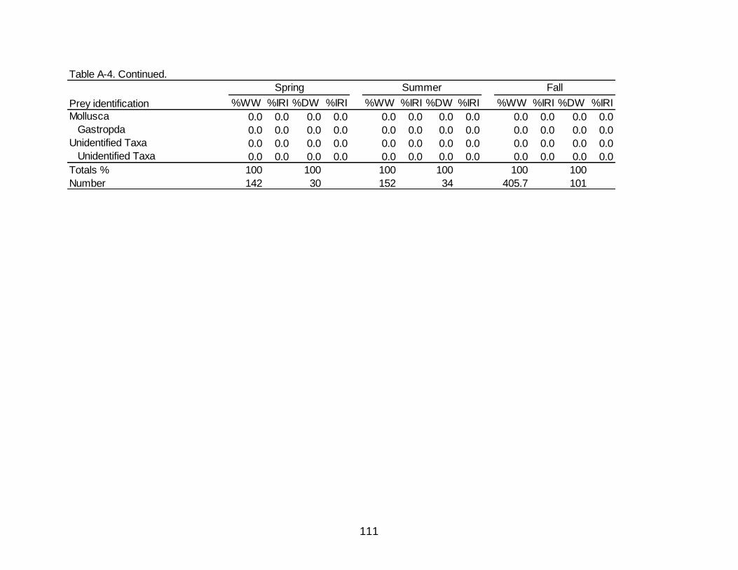
111
%WW %IRI %DW %IRI %WW %IRI %DW %IRI %WW %IRI %DW %IRI
0.0 0.0 0.0 0.0 0.0 0.0 0.0 0.0 0.0 0.0 0.0 0.0
0.0 0.0 0.0 0.0 0.0 0.0 0.0 0.0 0.0 0.0 0.0 0.0
0.0 0.0 0.0 0.0 0.0 0.0 0.0 0.0 0.0 0.0 0.0 0.0
0.0 0.0 0.0 0.0 0.0 0.0 0.0 0.0 0.0 0.0 0.0 0.0
Totals % 100 100 100 100 100 100
Number 142 30 152 34 405.7 101
Mollusca
Gastropda
Unidentified Taxa
Unidentified Taxa
Spring FallSummer
Prey identification
Table A-4. Continued.
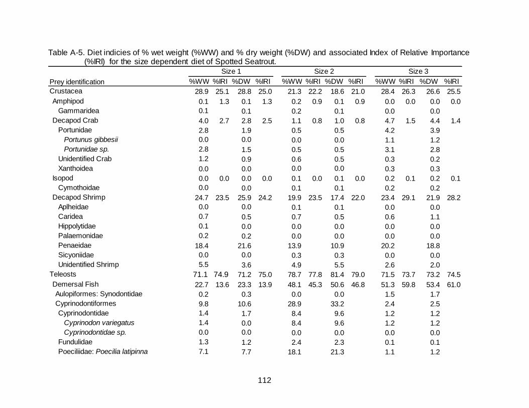
112
Table A-5. Diet indicies of % wet weight (%WW) and % dry weight (%DW) and associated Index of Relative Importance (%IRI) for the size dependent diet of Spotted Seatrout.
%WW %IRI %DW %IRI %WW %IRI %DW %IRI %WW %IRI %DW %IRI
28.9 25.1 28.8 25.0 21.3 22.2 18.6 21.0 28.4 26.3 26.6 25.5
0.1 1.3 0.1 1.3 0.2 0.9 0.1 0.9 0.0 0.0 0.0 0.0
0.1 0.1 0.2 0.1 0.0 0.0
4.0 2.7 2.8 2.5 1.1 0.8 1.0 0.8 4.7 1.5 4.4 1.4
2.8 1.9 0.5 0.5 4.2 3.9
Portunus gibbesii 0.0 0.0 0.0 0.0 1.1 1.2
Portunidae sp. 2.8 1.5 0.5 0.5 3.1 2.8
1.2 0.9 0.6 0.5 0.3 0.2
0.0 0.0 0.0 0.0 0.3 0.3
0.0 0.0 0.0 0.0 0.1 0.0 0.1 0.0 0.2 0.1 0.2 0.1
0.0 0.0 0.1 0.1 0.2 0.2
24.7 23.5 25.9 24.2 19.9 23.5 17.4 22.0 23.4 29.1 21.9 28.2
0.0 0.0 0.1 0.1 0.0 0.0
0.7 0.5 0.7 0.5 0.6 1.1
0.1 0.0 0.0 0.0 0.0 0.0
0.2 0.2 0.0 0.0 0.0 0.0
18.4 21.6 13.9 10.9 20.2 18.8
0.0 0.0 0.3 0.3 0.0 0.0
5.5 3.6 4.9 5.5 2.6 2.0
71.1 74.9 71.2 75.0 78.7 77.8 81.4 79.0 71.5 73.7 73.2 74.5
22.7 13.6 23.3 13.9 48.1 45.3 50.6 46.8 51.3 59.8 53.4 61.0
0.2 0.3 0.0 0.0 1.5 1.7
9.8 10.6 28.9 33.2 2.4 2.5
1.4 1.7 8.4 9.6 1.2 1.2
Cyprinodon variegatus 1.4 0.0 8.4 9.6 1.2 1.2
Cyprinodontidae sp. 0.0 0.0 0.0 0.0 0.0 0.0
1.3 1.2 2.4 2.3 0.1 0.1
7.1 7.7 18.1 21.3 1.1 1.2Poeciliidae: Poecilia latipinna
Teleosts
Demersal Fish
Aulopiformes: Synodontidae
Cyprinodontiformes
Cyprinodontidae
Fundulidae
Unidentified Shrimp
Unidentified Crab
Xanthoidea
Isopod
Cymothoidae
Decapod Shrimp
Aplheidae
Caridea
Hippolytidae
Palaemonidae
Penaeidae
Sicyoniidae
Size 3
Crustacea
Amphipod
Gammaridea
Decapod Crab
Portunidae
Prey identification
Size 1 Size 2
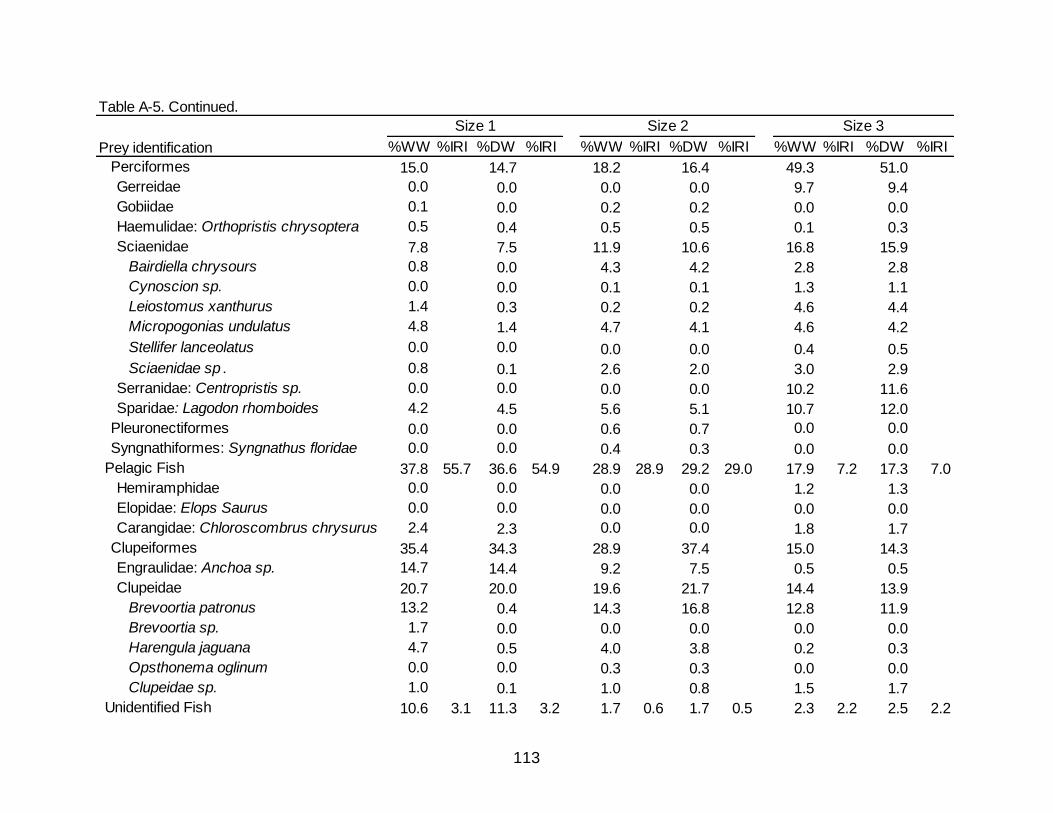
113
%WW %IRI %DW %IRI %WW %IRI %DW %IRI %WW %IRI %DW %IRI
15.0 14.7 18.2 16.4 49.3 51.0
0.0 0.0 0.0 0.0 9.7 9.4
0.1 0.0 0.2 0.2 0.0 0.0
0.5 0.4 0.5 0.5 0.1 0.3
7.8 7.5 11.9 10.6 16.8 15.9
Bairdiella chrysours 0.8 0.0 4.3 4.2 2.8 2.8
Cynoscion sp. 0.0 0.0 0.1 0.1 1.3 1.1
Leiostomus xanthurus 1.4 0.3 0.2 0.2 4.6 4.4
Micropogonias undulatus 4.8 1.4 4.7 4.1 4.6 4.2
Stellifer lanceolatus 0.0 0.0 0.0 0.0 0.4 0.5
Sciaenidae sp . 0.8 0.1 2.6 2.0 3.0 2.9
0.0 0.0 0.0 0.0 10.2 11.6
4.2 4.5 5.6 5.1 10.7 12.0
0.0 0.0 0.6 0.7 0.0 0.0
0.0 0.0 0.4 0.3 0.0 0.0
37.8 55.7 36.6 54.9 28.9 28.9 29.2 29.0 17.9 7.2 17.3 7.0
0.0 0.0 0.0 0.0 1.2 1.3
0.0 0.0 0.0 0.0 0.0 0.0
2.4 2.3 0.0 0.0 1.8 1.7
35.4 34.3 28.9 37.4 15.0 14.3
14.7 14.4 9.2 7.5 0.5 0.5
20.7 20.0 19.6 21.7 14.4 13.9
Brevoortia patronus 13.2 0.4 14.3 16.8 12.8 11.9
Brevoortia sp. 1.7 0.0 0.0 0.0 0.0 0.0
Harengula jaguana 4.7 0.5 4.0 3.8 0.2 0.3
Opsthonema oglinum 0.0 0.0 0.3 0.3 0.0 0.0
Clupeidae sp. 1.0 0.1 1.0 0.8 1.5 1.7
10.6 3.1 11.3 3.2 1.7 0.6 1.7 0.5 2.3 2.2 2.5 2.2
Sparidae: Lagodon rhomboides
Pleuronectiformes
Syngnathiformes: Syngnathus floridae
Pelagic Fish
Hemiramphidae
Elopidae: Elops Saurus
Carangidae: Chloroscombrus chrysurus
Clupeiformes
Engraulidae: Anchoa sp.
Clupeidae
Unidentified Fish
Serranidae: Centropristis sp.
Table A-5. Continued.
Prey identification
Size 1
Perciformes
Gerreidae
Gobiidae
Haemulidae: Orthopristis chrysoptera
Sciaenidae
Size 2 Size 3
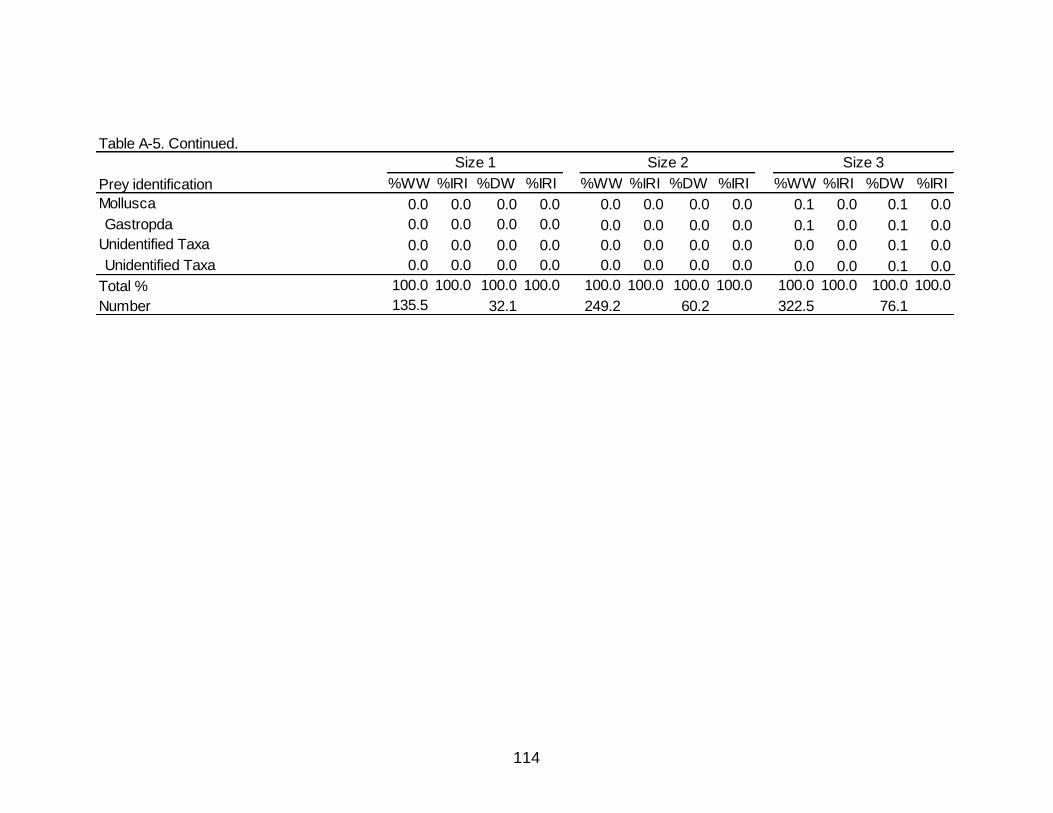
114
%WW %IRI %DW %IRI %WW %IRI %DW %IRI %WW %IRI %DW %IRI
0.0 0.0 0.0 0.0 0.0 0.0 0.0 0.0 0.1 0.0 0.1 0.0
0.0 0.0 0.0 0.0 0.0 0.0 0.0 0.0 0.1 0.0 0.1 0.0
0.0 0.0 0.0 0.0 0.0 0.0 0.0 0.0 0.0 0.0 0.1 0.0
0.0 0.0 0.0 0.0 0.0 0.0 0.0 0.0 0.0 0.0 0.1 0.0
100.0 100.0 100.0 100.0 100.0 100.0 100.0 100.0 100.0 100.0 100.0 100.0
135.5 32.1 249.2 60.2 322.5 76.1
Unidentified Taxa
Unidentified Taxa
Total %
Number
Prey identification
Size 1 Size 2 Size 3
Mollusca
Gastropda
Table A-5. Continued.
115
LIST OF REFERENCES
Abele, L. G., and W. Kim. 1986. An illustrated guide to the marine decapod crustaceans
of Florida. State of Florida Department of Environmental Regulation, Technical Series, 8(1).
Able, K. W., P. C. López-Duarte, F. J. Fodrie, O. P. Jensen, C. W. Martin, B. J. Roberts,
J. Valenti, K. O’Connor, and S. C. Halbert. 2014. Fish assemblages in Louisiana
salt marshes: Effects of the Macondo oil spill. Estuaries and Coasts:1-14.
Adkins, G., J. Tarver, P. Bowman, and B. Savoie. 1979. A study of the commercial finfish in coastal Louisiana. Louisiana Department of Wildlife and Fisheries Technical Bulletin Number 29. 87 p.
Akin, S., Winemiller, K. O., & Gelwick, F. P. 2003. Seasonal and spatial variations in fish
and macrocrustacean assemblage structure in Mad Island Marsh estuary, Texas. Estuarine, Coastal and Shelf Science, 57(1), 269-282.
Alanärä, A. and E. Brännäs. 1997. Diurnal and nocturnal feeding activity in arctic char and rainbow trout. Canadian Journal of Fisheries and Aquatic Sciences 54: 2894-
2900. Alonso, M. K., E. A. Crespo, N. A. García, S. N. Pedraza, P. A. Mariotti, and N. J. Mora.
2002. Fishery and ontogenetic driven changes in the diet of the Spiny Dogfish, Squalus acanthias, in Patagonian waters, Argentina. Environmental Biology of
Fishes 63(2):193-202. Atlas, R. M., D. M. Stoeckel, S. A. Faith, A. Minard-Smith, J. R. Thorn, and M. J.
Benotti. 2015. Oil Biodegradation and Oil-degrading Microbial Populations in Marsh Sediments Impacted by Oil from the Deepwater Horizon Well Blowout.
Environmental science & technology. Baker Jr, W. B., and G. Matlock. 1993. Movement of spotted seatrout tagged in Trinity
Bay, Texas. Northeast Gulf Science 13(1):29-34.
Baltz, D. M., C. Rakocinski, and J. W. Fleeger. 1993. Microhabitat use by marsh-edge fishes in a Louisiana estuary. Environmental Biology of Fishes 36(2):109-126.
Baremore, I. E., and D. M. Bethea. 2010. A guide to otoliths from fishes of the Gulf of Mexico. NOAA Technical Memorandum, NMFS-SEFSC-599.
Baremore, I. E. 2007. Feeding ecology of the Atlantic angel shark in the northeastern
Gulf of Mexico. Master’s thesis, Department of Fisheries and Aquatic Sciences,
University of Florida, Gainesville, Florida.
116
Barnes, B. T. 2014. Seasonal Differences in Diet of Two Predatory Fishes in Relation to Reef Type in the Inshore Northern Gulf of Mexico. Master's thesis. University of
Southern Mississippi, Hattiesburg, Mississippi.
Bedee, C. D., D. A. DeVries, S. A. Bortone, and C. L. Palmer. 2003. Estuary-specific age and growth of spotted seatrout in the northern Gulf of Mexico. Pages 57-77 in S. A. Bortone, editor. Biology of the spotted seatrout. CRC Press, Boca Raton,
FL.
Berens, E. J. 2005. Gastric evacuation and digestion state indices for gag, Mycteroperca microlepis, consuming fish and crustacean prey. Master’s thesis, Department of Fisheries and Aquatic Sciences, University of Florida, Gainesville,
Florida.
Bergman, E., and L. A. Greenberg. 1994. Competition between a planktivore, a benthivore, and a species with ontogenetic diet shifts. Ecology:1233-1245.
Bodkin, J., B. Ballachey, T. Dean, A. Fukuyama, S. Jewett, L. McDonald, D. Monson, C. O'Clair, and G. VanBlaricom. 2002. Sea otter population status and the process
of recovery from the 1989 Exxon Valdez' oil spill. Marine Ecology Progress Series 241(237):253.
Bowen, S. H., and D. R. Allanson. 1982. Behavioral and trophic plasticity of juvenile Tilapia mossambica in utilization of the unstable littoral habitat. Environmental
Biology of Fishes 7:357-362. Bowen, S. H. 1996. Quantitative description of the diet. Pages 513-529 in B.R. Murphy
and D.W. Willis, editors. Fisheries Techniques, 2nd edition. American Fisheries
Society, Bethesda, Maryland.
Bowling, B. 2012. Identification guide to marine organisms of Texas. Texas Parks and
Wildlife Department. Available: http://txmarspecies.tamug.edu/ (May 2017).
Bragg, J. R., R. C. Prince, E. J. Harner, and R. M. Atlas. 1994. Effectiveness of
bioremediation for the Exxon Valdez oil spill. Nature 368:413–418. Bromley, P.J. 1994. The role of gastric evacuation experiments in quantifying the
feeding rates of predatory fish. Reviews in Fish Biology and Fisheries 4:36-66.
Brown-Peterson, N. J., M. S. Peterson, D. L. Nieland, M. D. Murphy, R. G. Taylor, and J. R. Warren. 2002. Reproductive biology of female spotted seatrout, Cynoscion nebulosus, in the Gulf of Mexico: differences among estuaries? Environmental
Biology of Fishes 63(4):405-415.
117
Brown-Peterson, N. J., and J. W. Warren. 2001. The reproductive biology of spotted seatrout, Cynoscion nebulosus, along the Mississippi Gulf Coast. Gulf of Mexico
Science 19(1):61-73.
Brown, N., and R. Arnolos. 1988. Reproductive Biology of the Spotted Seatrout, Cynoscion nebulosus, in South Texas. Fishery Bulletin 86(2).
Bue, B. G., S. Sharr, and J. E. Seeb. 1998. Evidence of damage to pink salmon populations inhabiting Prince William Sound, Alaska, two generations after the
Exxon Valdez oil spill. Transactions of the American Fisheries Society 127(1):35-43.
Carpenter, K. E., editor. 2002. The living marine resources of the Western Central Atlantic. Rome: FAO.
Carr, W. E., and C. A. Adams. 1973. Food habits of juvenile marine fishes occupying
seagrass beds in the estuarine zone near Crystal River, Florida. Transactions of
the American Fisheries Society 102(3):511-540.
Carriger, J. F., and M. G. Barron. 2011. Minimizing risks from spilled oil to ecosystem services using influence diagrams: The Deepwater Horizon spill response. Environmental science & technology 45(18):7631-7639.
Cheek, A. O., C. A. Landry, S. L. Steele, and S. Manning. 2009. Diel hypoxia in marsh
creeks impairs the reproductive capacity of estuarine fish populations. Marine Ecology-Progress Series 392:211-221.
Chesney, E. J., D. M. Baltz, and R. G. Thomas. 2000. Louisiana estuarine and coastal fisheries and habitats: Perspectives from a fish's eye view. Ecological
Applications 10(2):350-366. Christensen, V., and C. J. Walters. 2004. Ecopath with Ecosim: methods, capabilities
and limitations. Ecological modelling 172(2):109-139.
Clarke, K. R., & Gorley, R. N. 2006. PRIMER V6: user manual-tutorial. Plymouth Marine Laboratory.
Clarke, K.R., and R.M. Warwick. 2001. Change in marine communities: an approach to statistical analysis and interpretation, 2nd edition. PRIMER-E: Plymouth
Comp, G., and W. Seaman Jr. 1985. Estuarine habitat and fishery resources of Florida.
Florida Aquatic Habitat and Fishery Resources:337-435.
Cortés, E. 1997. A critical review of methods of studying fish feeding based on analysis
of stomach contents: application to elasmobranch fishes. Canadian Journal of Fisheries and Aquatic Sciences 54(3):726-738.
118
Darnell, R. M. 1958. Food Habits of Fishes and Larger Invertebrat of Lake
Pontchartrain, Louisiana, an Estuarine Community. publications of the Institute of Marine Science 5:353-416.
Dubansky, B., A. Whitehead, J. T. Miller, C. D. Rice, and F. Galvez. 2013. Multitissue
molecular, genomic, and developmental effects of the Deepwater Horizon oil spill
on resident Gulf killifish (Fundulus grandis). Environmental science & technology 47(10):5074-5082.
Eggleston, D. B., J. J. Grover, and R. N. Lipcius. 1998. Ontogenetic diet shifts in
Nassau grouper: trophic linkages and predatory impact. Bulletin of Marine
Science 63(1):111-126.
Esler, D., A. Schmutz, and L. Jarvis. 2000. Winter survival of adult female harlequin ducks in relation to history of contamination by the Exxon Valdez oil spill. Journal of Wildlife Management 64:839-847.
Fodrie, F., and K. Heck Jr. 2011. Response of Coastal Fishes to the Gulf of Mexico Oil
Disaster. PloS one 6(7):e21609. Fraser, N. H. C., N. B. Metcalfe, and J.E. Thorpe. 1993. Temperature-dependent switch
between diurnal and nocturnal foraging in salmon. Proceedings of the Royal Society of London Series B 252: 135-139.
Fraser, N. H. C., J. Heggenes, N. B. Metcalfe, and J. E. Thorpe. 1995. Low summer
temperatures cause juvenile Atlantic salmon to become nocturnal. Canadian
Journal of Zoology 73: 446-451. Fulton, E. A., J. S. Link, I. C. Kaplan, M. Savina‐Rolland, P. Johnson, C. Ainsworth, P.
Horne, R. Gorton, R. J. Gamble, and A. D. Smith. 2011. Lessons in modelling
and management of marine ecosystems: the Atlantis experience. Fish and Fisheries 12(2):171-188.
Galarowicz, T. L., J. A. Adams, and D. H. Wahl. 2006. The influence of prey availability
on ontogenetic diet shifts of a juvenile piscivore. Canadian Journal of Fisheries
and Aquatic Sciences 63(8):1722-1733.
Garvey, J. E., and S. R. Chipps. 2013. Diets and Energy Flow. Pages 733-772 in A. V. Zale, D. L. Parrish, and T. M. Sutton, editors. Fisheries Techniques. American Fisheries Society, Bethesda, MD.
Gosselink, J. G. 1984. The ecology of delta marshes of coastal Louisiana: a community
profile. Pages 134 in. U.S. Fish & Wildlife Service.
119
Graham, B., W. K. Reilly, F. Beinecke, D. F. Boesch, T. D. Garcia, C. A. Murray, and F. Ulmer. 2011. Deep Water: The Gulf Oil Disaster And The Future Of Offshore
Drilling. Report to the President: National Commission on the BP Deepwater Horizon Oil Spill Offshore Drilling. US Government Printing Office, Washington,
DC. Gunter. 1945. Studies on Marine Fishes of Texas. publications of the Institute of Marine
Science 1(1):76-78.
Härkönen, T. 1986. Guide to the otoliths of the bony fishes of the Northeast Atlantic. Hellerup: Danbiu.
Hein, S., and J. Shepard. 1979. Spawning of spotted seatrout in a Louisiana estuarine ecosystem. Proceedings of the annual conference-Southeastern Association of
Fish and Wildlife Agencies. Heintz, R. A., J. W. Short, and S. D. Rice. 1999. Sensitivity of fish embryos to
weathered crude oil: Part II. Increased mortality of pink salmon (Oncorhynchus gorbuscha) embryos incubating downstream from weathered Exxon Valdez
crude oil. Environmental Toxicology and Chemistry 18(3):494-503. Hendon, J., J. Warren, J. Franks, and M. Buchanan. 2002. Movements of Spotted
Seatrout (Cynoscion nebulosus) in Mississippi coastal waters based on tag-recapture. Gulf of Mexico Science 20(2):91-97.
Herdter, E. S., Chambers, D. P., Stallings, C. D., & Murawski, S. A. (2017). Did the
Deepwater Horizon oil spill affect growth of Red Snapper in the Gulf of Mexico?
Fisheries Research, 191, 60-68.
Hettler Jr, W. F. 1989. Food habits of juveniles of spotted seatrout and gray snapper in western Florida Bay. Bulletin of Marine Science 44(1):155-162.
Houde, E. D., and J. A. Lovda. 1984. Seasonality of occurrence, foods and food preferences of ichthyoplankton in Biscayne Bay, Florida. Estuarine, Coastal and
Shelf Science 18(4):403-419. Hyslop, E. 1980. Stomach contents analysis—a review of methods and their application.
Journal of fish biology 17(4):411-429.
Ihde, T. F., and Chittenden, M. E. 2002. Comparison of calcified structures for aging spotted seatrout. Transactions of the American Fisheries Society, 131(4), 634-642.
Incardona, J. P., L. D. Gardner, T. L. Linbo, T. L. Brown, A. J. Esbaugh, E. M. Mager, J.
D. Stieglitz, B. L. French, J. S. Labenia, and C. A. Laetz. 2014. Deepwater
120
Horizon crude oil impacts the developing hearts of large predatory pelagic fish. Proceedings of the National Academy of Sciences 111(15):E1510-E1518.
Iversen, E. S., and D. C. Tabb. 1962. Subpopulations based on growth and tagging
studies of Spotted Seatrout, Cynoscion nebulosus, in Florida. Copeia:544-548. Johnson, J. H., and D. S. Dropkin. 1993. Diel variation in diet composition of a riverine
fish community. Hydrobiologia 271:149-158.
Johnson, M. W., S. A. Bortone, B. W. Klement, and R. L. Shipp. 2011. Population changes and location-specific differences for otolith-derived age and growth of recreationally harvested Spotted Seatrout (Cynoscion nebulosus) from Alabama
in 2007. Gulf of Mexico Science 29:13-24.
Jones, R.F., D.M. Baltz, and R.L. Allen. 2002. Patterns of resource use by fishes and macroinvertebrates in Barataria Bay, Louisiana. Marine Ecology Progress Series 237:271-289
Kells, V. and K. Carpenter. 2011. A field guide to coastal fishes from Maine to Texas.
The John Hopkins University Press. Baltimore, MD. Kennedy, C. J., and S.-M. Cheong. 2013. Lost ecosystem services as a measure of oil
spill damages: a conceptual analysis of the importance of baselines. Journal of environmental management 128:43-51.
Kingston, P. F. 2002. Long-term environmental impact of oil spills. Spill Science &
Technology Bulletin 7(1):53-61.
Kneib, R. T. 1997. The role of tidal marshes in the ecology of estuarine nekton.
Oceanography and Marine Biology 35:163-220. Krebs CJ . 1999. Ecological Methodology, 2nd edn. Menlo Park, CA: Addison-Wesley
Longman
Krebs, C. J., S. Boutin, R. Boonstra, A. Sinclair, J. Smith, M. R. Dale, K. Martin, and R. Turkington. 1995. Impact of food and predation on the snowshoe hare cycle. Science 269(5227):1112-1115.
Latour, R. J., M. J. Brush, and C. F. Bonzek. 2003. Toward ecosystem-based fisheries
management: strategies for multispecies modeling and associated data requirements. Fisheries 28(9):10-22.
Levy, J. K., and C. Gopalakrishnan. 2010. Promoting ecological sustainability and community resilience in the US Gulf Coast after the 2010 Deepwater Horizon oil
spill. Journal of Natural Resources Policy Research 2(3):297-315.
121
Lin, Q., and I. A. Mendelssohn. 2012. Impacts and recovery of the Deepwater Horizon oil spill on vegetation structure and function of coastal salt marshes in the
northern Gulf of Mexico. Environmental science & technology 46(7):3737-3743.
Lindeman, R. L. 1942. The trophic-dynamic aspect of ecology. Ecology 23(4):399-417. Link, J. S., and L. P. Garrison. 2002. Trophic ecology of Atlantic cod Gadus morhua on
the northeast US continental shelf. Marine Ecology Progress Series 227:109-123.
Livingston, R. J. 1976. Diurnal and seasonal fluctuations of organisms in a north Florida
estuary. Estuarine and Coastal Marine Science 4, 373–400.
Livingston, R. J. 1990. Inshore marine habitats. Pages 549-573 in R. L. Myers, and J. J.
Ewel, editors. Ecosystems of Florida. University of Central Florida Press, Orlando, FL.
Llanso, R. J., S. S. Bell, and F. E. Vose. 1998. Food habits of red drum and spotted seatrout in a restored mangrove impoundment. Estuaries 21(2):294-306.
Mason, W., and S. Zengel. 1996. Foods of juvenile spotted seatrout in seagrasses at
Seahorse Key, Florida. Gulf of Mexico Science 14:89-104.
Mathur, D. 1977. Food habits and competitive relationships of the bandfin shiner in
Halawakee Creek, Alabama. The American Midland Naturalist 97:89-100. McCall, B. D., & Pennings, S. C. (2012). Disturbance and recovery of salt marsh
arthropod communities following BP Deepwater Horizon oil spill. PloS one, 7(3), e32735.
McCann, M.J., Able, K.W., Christian, R.R., Fodrie, F.J., Jensen, O.P., Johnson, J.J.,
López‐Duarte, P.C., Martin, C.W., Olin, J.A., Polito, M.J. and Roberts, B.J. 2017.
Key taxa in food web responses to stressors: the Deepwater Horizon oil spill.
Frontiers in Ecology and the Environment 15(3):142-149. McCormick, M. 1998. Ontogeny of diet shifts by a microcarnivorous fish, Cheilodactylus
spectabilis: relationship between feeding mechanics, microhabitat selection and growth. Marine Biology 132(1):9-20.
McErlean, A. J., O’Connor, S. G., Mihursky, J. A., & Gibson, C. I. 1973. Abundance,
diversity and seasonal patterns of estuarine fish populations. Estuarine and
Coastal Marine Science 1, 19–36. McMichael, R. H., and K. M. Peters. 1989. Early life history of spotted seatrout,
Cynoscion nebulosus (Pisces: Sciaenidae), in Tampa Bay, Florida. Estuaries 12(2):98-110.
122
McMichael, R. H., K. M. Peters, and G. R. Parsons. 1989. Early life history of the
snook, Centropomus undecimalis, in Tampa Bay, Florida. Northeast Gulf Science 10: 113-125.
McNutt, M. K., R. Camilli, T. J. Crone, G. D. Guthrie, P. A. Hsieh, T. B. Ryerson, O.
Savas, and F. Shaffer. 2012. Review of flow rate estimates of the Deepwater
Horizon oil spill. Proceedings of the National Academy of Sciences 109(50):20260-20267.
McNutt, M. K., R. Camilli, G. D. Guthrie, P. A. Hsieh, V. F. Labson, W. J. Lehr, D.
Maclay, A. C. Ratzel, and M. K. Sogge. 2011. Assessment of flow rate estimates
for the Deepwater Horizon/Macondo well oil spill. Flow Rate Technical Group report to the National Incident Command, Interagency Solutions Group.
Mendelssohn, I. A., G. L. Andersen, D. M. Baltz, R. H. Caffey, K. R. Carman, J. W.
Fleeger, S. B. Joye, Q. Lin, E. Maltby, and E. B. Overton. 2012. Oil impacts on
coastal wetlands: implications for the Mississippi River Delta ecosystem after the Deepwater Horizon oil spill. BioScience 62(6):562-574.
Metcalfe, N. B., N. H. C. Fraser, and M. D. Burns. 1998. State-dependent shifts
between nocturnal and diurnal foraging in salmon. Proceedings of the Royal
Society of London Series B 265: 1503-1507.
Michel, J., E. H. Owens, S. Zengel, A. Graham, Z. Nixon, T. Allard, W. Holton, P. D. Reimer, A. Lamarche, and M. White. 2013. Extent and degree of shoreline oiling: Deepwater Horizon oil spill, Gulf of Mexico, USA. PloS one 8(6):e65087.
Miles, D. W. 1950. Life Histories of the Spotted Sea Trout, Cynoscion nebulosus, and
the Redfish, Sciaenops ocellatus. Texas Game and Fish Commission, Marine Labratory Annual Report, 1949-1950.
Minello, T. J., & Zimmerman, R. J. 1983. Fish predation on juvenile brown shrimp, Penaeus aztecus Ives: The effect of simulated Spartina structure on predation
rates. Journal of Experimental Marine Biology and Ecology 72(3):211-231. Minello, T. J., & Zimmerman, R. J. 1991. The role of estuarine habitats regulating
growth and survival of juvenile penaeid shrimp. In P. DeLoach, W. J. Doughherty, & M. A. Davidson (Eds.), Frontiers in shrimp research (pp. 1–16). Amsterdam:
Elsevier. Mol, J. 1995. Ontogenetic diet shifts and diet overlap among three closely related
neotropical armoured catfishes. Journal of Fish Biology 47(5):788-807.
123
Moody, W. D. 1950. A study of the natural history of spotted seatrout, Cynoscion nebulosus, in the Cedar Key, Florida area. Quarterly Journal of the Florida
Academy of Science, 12:147-171
Murie, D. 1995. Comparative feeding ecology of two sympatric rockfish congeners, Sebastes caurinus (copper rockfish) and S. maliger (quillback rockfish). Marine Biology 124(3):341-353.
Murie, D. J., and D. Lavigne. 1985. A technique for the recovery of otoliths from
stomach contents of piscivorous pinnipeds. The Journal of Wildlife Management:910-912.
Murphy, M. D., and R. G. Taylor. 1994. Age, growth, and mortality of spotted seatrout in Florida waters. Transactions of the American Fisheries Society 123(4):482-497.
NMFS (National Marine Fisheries Service). 2014. Fisheries Economics of the Unites
States, 2012. Pages 175 in N. U.S. Department of Commerce, editor.
NOAA (National Oceanic and Atmospheric Administration) and UNH CRRC (University
of New Hampshire Coastal Response Research Center). 2012. ERMA (Environmental Resource Management Application). Available: http://gomex.erma.noaa.gov/erma.html. (February 2017).
Nieland, D. L., R. G. Thomas, and C. A. Wilson. 2002. Age, growth, and reproduction of
spotted seatrout in Barataria Bay, Louisiana. Transactions of the American Fisheries Society 131(2):245-259.
Norberg, M. J. (2015). The ecology of tomtate, Haemulon aurolineatum, in the northern Gulf of Mexico and effects of the Deepwater Horizon oil spill. University of South
Alabama. Olson, M. H. 1996. Ontogenetic niche shifts in largemouth bass: variability and
consequences for first-year growth. Ecology:179-190.
Overstreet, R. M. 1983. Aspects of the biology of the spotted seatrout, Cynoscion nebulosus, in Mississippi. Gulf and Caribbean Research 7(5):1-43
Pauly, D., V. Christensen, and C. Walters. 2000. Ecopath, Ecosim, and Ecospace as tools for evaluating ecosystem impact of fisheries. ICES Journal of Marine
Science: Journal du Conseil 57(3):697-706. Pazzia, I., M. Trudel, M. Ridgway, and J. B. Rasmussen. 2002. Influence of food web
structure on the growth and bioenergetics of lake trout (Salvelinus namaycush). Canadian Journal of Fisheries and Aquatic Sciences 59(10):1593-1605.
124
Pearson, J. C. 1929. Natural history and conservation of the redfish and other commercial sciaenids on the Texas coast. Bulletin of the U.S Bureau of Fisheries
(64):178-194.
Perret, W. S., J. Weaver, R. Williams, P. Johansen, T. McIlwain, R. Raulerson, and W. Tatum. 1980. Fishery profiles of red drum and spotted seatrout. Gulf States Marine Fisheries Commission 6.
Persson, L. 1988. Asymmetries in competitive and predatory interactions in fish
populations. In Size-structured populations (pp. 203-218). Springer Berlin Heidelberg.
Persson, A., and L.-A. Hansson. 1999. Diet shift in fish following competitive release. Canadian Journal of Fisheries and Aquatic Sciences 56(1):70-78.
Peterson, C. H., S. D. Rice, J. W. Short, D. Esler, J. L. Bodkin, B. E. Ballachey, and D.
B. Irons. 2003. Long-term ecosystem response to the Exxon Valdez oil spill.
Science 302(5653):2082-2086.
Peterson, G., and R. Turner. 1994. The value of salt marsh edge vs interior as a habitat for fish and decapod crustaceans in a Louisiana tidal marsh. Estuaries 17(1):235-262.
Pilcher, W., S. Miles, S. Tang, G. Mayer, and A. Whitehead. 2014. Genomic and
Genotoxic Responses to Controlled Weathered-Oil Exposures Confirm and Extend Field Studies on Impacts of the Deepwater Horizon Oil Spill on Native Killifish. PloS one 9(9).
Pinkas, L. 1971. Food habits study. Fishery Bulletin 152:5-10.
Renones, O., N. Polunin, and R. Goni. 2002. Size related dietary shifts of Epinephelus
marginatus in a western Mediterranean littoral ecosystem: an isotope and
stomach content analysis. Journal of fish biology 61(1):122-137.
Rice, S. D., R. E. Thomas, M. G. Carls, R. A. Heintz, A. C. Wertheimer, M. L. Murphy, J. W. Short, and A. Moles. 2001. Impacts to pink salmon following the Exxon Valdez oil spill: persistence, toxicity, sensitivity, and controversy. Reviews in
Fisheries Science 9(3):165-211.
Richards, T. M. 2014. Trophic Dynamics of Spotted Seatrout (Cynoscion nebulosus) in a River-Dominated Coastal Estuary, Apalachicola Bay, Florida. Master's thesis. Florida State University, Tallahassee, Florida.
Robinette, H.R. 1983. Species profiles: Life histories and environmental requirements of
125
coastal fishes and invertebrates (Gulf of Mexico) – bay anchovy and striped anchovy. L1S. Fish and Wildlife Service, Division of Biological Services,
FWS/OBS-82/11.14. U. S. Army Corps of Engineers, TR EL-82-4. 15 pp.
Rock, J.E. 2009. Summer feeding ecology of juvenile Common Snook in southwest Florida tidal creeks. Master’s thesis, Department of Fisheries and Aquatic Sciences, University of Florida, Gainesville, Florida.
Rozas, L. P., T. J. Minello, and M. S. Miles. 2014. Effect of Deepwater Horizon oil on
growth rates of juvenile penaeid shrimps. Estuaries and Coasts 37(6):1403-1414. Russell, M. 2005. Spotted Sea Trout (Cynoscion nebulosus) and Pinfish (Lagodon
Rhomboides) Dietary Analysis According to Habitat Type. Master's thesis. Louisiana State University, Baton Rouge, Louisiana.
Sánchez-Vázquez, F. J., J. A. Madrid, and S. Zamora. 1995. Circadian rhythms of
feeding activity in sea bass, Dicentrarchus labrax. dual phasing capacity of diel
demand- feeding pattern. Journal of Biological Rhythms 10: 256-266.
Scarratt, D. J., and V. Zitko. 1972. Bunker C oil in sediments and benthic animals from shallow depths in Chedabucto Bay, N.S.J. Fish. Res. Board Can. 29:1345-1350.
Scharf, F. S., Juanes, F., & Rountree, R. A. 2000. Predator size-prey size relationships of marine fish predators: interspecific variation and effects of ontogeny and body
size on trophic-niche breadth. Marine Ecology Progress Series, 208, 229-248. Silliman, B. R., J. Van de Koppel, M. D. Bertness, L. E. Stanton, and I. A. Mendelssohn.
2005. Drought, snails, and large-scale die-off of southern US salt marshes. Science 310(5755):1803-1806.
Silliman, B. R., J. van de Koppel, M. W. McCoy, J. Diller, G. N. Kasozi, K. Earl, P. N.
Adams, and A. R. Zimmerman. 2012. Degradation and resilience in Louisiana
salt marshes after the BP–Deepwater Horizon oil spill. Proceedings of the National Academy of Sciences 109(28):11234-11239.
Simonsen, K. A. 2008. The effect of an inshore artificial reef on the community structure
and feeding ecology of estuarine fishes in Barataria Bay, Louisiana. Master's
thesis. Louisiana State University, Baton Rouge, Louisiana.
Simonsen, K. A., J.H. Cowan. 2008. Sport fish utilization of an inshore artificial oyster reef in Barataria Bay, Louisiana. In: Proceedings of the Gulf and Caribbean Fisheries Institute, 60: 389-406.
Simonsen, K. A., J.H. Cowan. 2013. Examination of an estuarine fish assemblage over
an inshore artificial reef. Open Fish Science Journal, 6, 48-57
126
Stetter, S. P., L. Witzel, L. Rudstam, D. Einhouse, and E. Mills. 2005. Energetic consequences of diet shifts in Lake Erie rainbow smelt (Osmerus mordax).
Canadian Journal of Fisheries and Aquatic Sciences 62(1):145-152.
Tabb, D. C. 1966. The estuary as a habitat for spotted seatrout, Cynoscion nebulosus. American Fisheries Society Special Publication (3):58-67.
Tarnecki, J. H., and W. F. Patterson III. 2015. Changes in Red Snapper Diet and Trophic Ecology Following the Deepwater Horizon Oil Spill. Marine and Coastal
Fisheries 7(1):135-147. Teal, J. M., and R. W. Howarth. 1984. Oil spill studies: a review of ecological effects.
Environmental Management 8(1):27-43.
Tomasko, D., C. Corbett, H. Greening, and G. Raulerson. 2005. Spatial and temporal variation in seagrass coverage in Southwest Florida: assessing the relative effects of anthropogenic nutrient load reductions and rainfall in four contiguous
estuaries. Marine Pollution Bulletin 50(8):797-805.
Turner, R. E., E. B. Overton, B. M. Meyer, M. S. Miles, G. McClenachan, L. Hooper-Bui, A. S. Engel, E. M. Swenson, J. M. Lee, and C. S. Milan. 2014. Distribution and recovery trajectory of Macondo (Mississippi Canyon 252) oil in Louisiana coastal
wetlands. Marine Pollution Bulletin 87(1):57-67.
USACE (U.S Army Corps of Engineers). 2004. Louisiana Coastal Area: Ecosystem Restoration Study. Available: https://www.lca.gov/Library/ProductList.aspx?ProdType=0&folder=1125 (May
2017)
Valdimarsson, S. K., S. Skúlason, and N. B. Metcalfe. 2000. Experimental demonstration of differences in sheltering behaviour between Icelandic populations of Atlantic salmon (Salmo salar) and Arctic char (Salvelinus alpinus).
Canadian Journal of Fisheries and Aquatic Sciences 57: 719-724.
Wallace, R. K. 1981. An Assessment of Diet-Overlap Indexes, Transactions of the American Fisheries Society, 110:1, 72-76.
Walters, C. J., & Martell, S. J. (2004). Fisheries ecology and management. Princeton University Press.
Walters, S., S. Lowerre-Barbieri, J. Bickford, and D. Mann. 2009. Using a passive
acoustic survey to identify spotted seatrout spawning sites and associated
habitat in Tampa Bay, Florida. Transactions of the American Fisheries Society 138(1):88-98.
127
Warren, C.E., and G.E. Davis. 1967. Laboratory studies on the feeding, bioenergetics, and growth of fish. Pages 175-214 in S.D. Gerking (Ed.). The biological basis of
freshwater fish production. Blackwell Sci. Pub., Oxford.
Whitehead, A., B. Dubansky, C. Bodinier, T. I. Garcia, S. Miles, C. Pilley, V. Raghunathan, J. L. Roach, N. Walker, and R. B. Walter. 2011. Genomic and physiological footprint of the Deepwater Horizon oil spill on resident marsh fishes.
Proceedings of the National Academy of Sciences:201109545.
Wieting, D. 1989. Life History and Population Dynamics of Spotted Seatrout (Cynoscion nebulosus) in Louisiana. Master's Thesis. Louisiana State University, Baton Rouge, Louisiana.
Winemiller, K. O. 1989. Ontogenetic diet shifts and resource partitioning among
piscivorous fishes in the Venezuelan ilanos. Environmental Biology of Fishes 26(3):177-199.
Winemiller, K. O. 1990. Spatial and temporal variation in tropical fish trophic networks. Ecological Monographs 60(3):331-367.
Zaret, T. M., and A. S. Rand. 1971. Competition in tropical stream fishes: support for the
com- petitive exclusion principle. Ecology 52:336-342.
Zein-Eldin, Z.P. and M.L. Renaud. 1986. Inshore environmental effects on brown
shrimp, Penaeus aztecus, and White shrimp, P. setiferus, populations in coastal waters, particularly in Texas. Marine Fisheries Review 48(3):9-15.
Zimmerman, R.J. and T.J. Minello. 1984. Densities of Penaeus aztecus, Penaeus setiferus, and other natant macrofauna in a Texas salt marsh. Estuaries.
7(4A):421-433.

128
BIOGRAPHICAL SKETCH
John, or Drew as he prefers to be called, got his itch for fish while growing up
fishing with his Dad and Grandpop on the Delaware River and down the Jersey Shore.
He left home in 2006 to attend the University of New England in southern Maine to
study marine biology. In 2008, Drew began working in fisheries research under the
guidance of Dr. James Sulikowski, who introduced him to the smelly world of shark diet
studies. He graduated with a Bachelor of Science degree in May 2010 and began work
as a fisheries biologist with NOAA Fisheries in Panama City Beach, FL, where he
worked for 3 years on the recovery and management of Gulf Sturgeon. Wanting to
further advance his career, Drew accepted a fisheries biologist position in the lab of Dr.
Debra Murie at the University of Florida, which soon turned into the current Master of
Science degree. Drew hopes to pursue a career in fisheries in which he can support the
biological research needed for stock assessments and the appropriate management of
fish populations.


![NASA March05.ppt [Read-Only] · Ichthyophis kohtaoensis Caeciliidae Dermophis mexicanus Typhlonectidae Typhlonectes sp. Caudata Hynobiidae Hynobius nebulosus Salamandridae Cynops](https://img.pdfslide.us/doc/110x75/5e591e05e1cb895875286147/nasa-read-only-ichthyophis-kohtaoensis-caeciliidae-dermophis-mexicanus-typhlonectidae.jpg)