© 2011 Shrenik Kothari

MODELING OF THE DYNAMICS OF AUTONOMOUS CATALYTIC NANOMOTORS

USING THE METHOD OF REGULARIZED STOKESLETS

BY

SHRENIK KOTHARI

THESIS

Submitted in partial fulfillment of the requirements

for the degree of Master of Science in Mechanical Engineering

in the Graduate College of the

University of Illinois at Urbana-Champaign, 2011

Urbana, Illinois

Adviser:

Professor David Saintillan

ii

Abstract

Catalytic nanomotors move autonomously by deriving energy directly from their

environment, mimicking biological nanomotors that perform a wide range of complex functions

at the cellular level and drive vital functions such as active transport, muscle contraction, cell

mobility, and other movement. With the belief that precise control of microscale and nanoscale

motors may eventually permit the design of functional machinery at these scales, researchers

have been systematically designing such nanomotors and experimentally investigating their

swimming behavior.

The complex nature of fluid-structure interaction resulting from complicated surface

geometry, the Brownian fluctuations and the contact surface effects, necessitate appropriate

theoretical modeling and use of computational methods and tools to accurately simulate particle

dynamics. The swimming behavior exhibited by catalytic nanomotors designed by Gibbs and

Zhao is numerically simulated based on an accurate representation of the nanomotor geometry,

full hydrodynamic interactions of the nanomotor components as well as with the supporting

substrate, accurately captured by the method of Regularized Stokeslets. We also account for

solid-frictional forces and torques from the substrate, as prescribed by an established velocity-

dependent friction model for micro/nanoscale friction. To explain random deviations, the

Brownian fluctuations are precisely modeled as the stochastic solution to a Langevin Equation

satisfying the fluctuation-dissipation theorem of statistical mechanics. A comparison of our

numerically simulated results with the experimental observations is also presented here.

iii

To my family …

iv

Acknowledgement

It is a great pleasure to thank everybody who made this thesis possible. I owe my deepest

gratitude to my advisor, Prof. David Saintillan since if it would not have been for his invaluable

guidance and constant support throughout the course of my research duration, this thesis would

not have reached its successful completion. I am especially grateful to him for always being

available to patiently answer my queries and doubts.

Also, as this project was a collaborative effort with John Gibbs and Dr. Yiping Zhao, I would

like to thank them for approaching us with this very interesting and challenging work based on

their experimental investigation of catalytic nanomotors. I would like to thank John Gibbs for

making himself available in providing all the necessary data and information pertaining to my

work.

I am indebted to FMC Technologies Inc. for awarding me their prestigious Fellowship over the

academic period 2010-2011, whereby taking care of my tuition and awarding me a substantial

stipend as well. Without their financial support it would not have been possible to dedicate my

efforts towards my thesis research as well as I finally could. I am also immensely grateful to the

Mechanical Science and Engineering Department for providing me this wonderful opportunity of

undertaking Graduate Studies at this highly esteemed institution, and also extending financial

support in the form of several Teaching Assistantship opportunities.

Last but not the least, I would like to express my deep gratitude to my parents Haresh Kothari

and Nayna Kothari and my brother Bhavik Kothari, for always believing in me and encouraging

me to pursue my goals.

v

Table of Contents

List of Figures…………………………………………………………………………………..vii

List of Tables…………………………………………………………………………………….ix

Chapter 1: Introduction ................................................................................................................1

Chapter 2: Experimental Investigation .....................................................................................10

2.1. Fabrication and Structural Study ........................................................................................10

2.2. Motion Characteristics ........................................................................................................13

2.2.1. Armlength effect .........................................................................................................15

2.2.2. Concentration effect ....................................................................................................17

2.2.3. Arm-inclination effect .................................................................................................17

Chapter 3: Hydrodynamic Modeling .........................................................................................19

3.1. Boundary Integral Methods ...............................................................................................19

3.2. Stokes Flow Modeling – Method of Regularized Stokeslets .............................................19

3.3. Numerical Computation of Mobility Matrix .....................................................................22

Chapter 4: Validation of the Method of Regularized Stokeslets .............................................26

4.1. Validation of the Image system for single particle wall Hydrodynamic interactions ........26

4.2. Validation of the Stokeslet system for pair Hydrodynamic interactions ............................30

Chapter 5: Mesh Generation ......................................................................................................38

Chapter 6: Nanomotor Dynamics – Modeling and Simulation ...............................................45

6.1. Modeling .............................................................................................................................45

6.2. Simulation ...........................................................................................................................46

Chapter 7: Simulation Results ....................................................................................................48

Chapter 8: Conclusion .................................................................................................................54

References .....................................................................................................................................56

Appendix A. Computed ‘Hydrodynamic Resistance’ Matrices .............................................58

vi

Appendix B. Brownian Fluctuation Modeling .........................................................................61

Appendix C. Contact Friction Modeling at Microscales ..........................................................64

Appendix D. Animated Simulation of Nanomotor Trajectories ..............................................71

vii

List of Figures

Figure 1.1: (a) Propulsion mechanism due to bubble ejection. (b) Scanning electron

micrograph of a Pt-coated spherical silica microbead [9]………………………………………...2

Figure 1.2: (a) Schematic of a silica microbead monolayer; (b) optical micrograph of

the monolayer under 40X magnification; (c) Ti and Pt evaporated onto the monolayer;

(d) SEM top-view of the monolayer with TiO2 arms; (e) and schematic of the deposition of

the TiO2 arms at a large angle [8]…………………………………………………………………3

Figure 1.3: Scanning electron micrographs of the structures removed from the substrate

with arms of various lengths: (a) 0 μm; (b) 1.25 μm; (c) 2.5 μm; (d) 3.75 μm; (e) 5 μm; (f)

and 6.25 μm [8]……………………………………………………………………………………4

Figure 1.4: Curvature κ (black) and angular frequency ω (red) vs. TiO2 arm length [8]………...5

Figure 1.5: (a) For the OAD sample, the speed is increased by increasing the concentration

of H2O2.(b) the GLAD sample shows significantly less increase in curvature with respect

to speed [8]…………………………………………………………………………………...........6

Figure 2.1: (a) SEM of GLAD-grown nanomotor with the TiO2 arm perpendicular to the

line separating the half-coated microbead; (b) and Schematic of the same [8]………………….13

Figure 2.2: Plot showing the trajectories of 4 different arm lengths. Each plot is a 10 s.

interval, and the centers of each trajectory have been deliberately moved to a mutual

middle [8]………………………………………………………………………………………...14

Figure 2.3: (a) Schematic of a GLAD-grown nanomotor; (b) SEM of a GLAD-grown

nanomotor after being removed by sonication [8]……………………………………………….18

Figure 4.1: Variation of drag force acting on sphere of radius 1 µm, translating parallel to

wall with speed U=1 µm/s, with distance from wall below……………………………………...27

Figure 4.2: Variation of drag torque acting on sphere of radius 1 µm, rotating about axis

normal to wall with angular speed equal to 1 rad/s, with distance from wall below…………….27

Figure 4.3: Variation of drag force (log) acting on prolate spheroid of major axis = 1.5µm,

minor axis =0.71 µm, translating parallel to wall along the major axis, with speed equal to

1 µm/s, with variation of separation distance from wall (log)…………………………………...28

Figure 4.4: Variation of drag force (log) acting on prolate spheroid of major axis = 1.5µm,

minor axis =0.71 µm, translating parallel to wall along the minor axis, with speed equal to

1 µm/s , with variation of separation distance from wall (log)…………………………………..29

Figure 4.5: Variation of the induced force on sphere s1 by sphere s2 translating

perpendicular to its line of centers, in unbounded flow as the distance of separation

between the pair is varied, computed using the Regularized Stokeslet method…………………36

Figure 4.6: Variation of the computed induced force on sphere s1 by sphere s2 translating

perpendicular to its line of centers, for different wall separation distances, as the distance

of separation between the pair is varied………………………………………………………….37

viii

Figure 5.1: Typical nanomotor geometry used in the simulations, shown with mesh

corresponding to an arm length of 3.5 µm (axes labels are in microns)........................................42

Figure 5.2: (a) Mesh generated for nanomotor of armlength 1.7μm; (b) Modeled structure

geometry for the same……………………………………………………………………………43

Figure 5.3: (a) Mesh generated for nanomotor of armlength 3.5 μm; (b) Modeled

structure geometry for the same………………………………………………………………….43

Figure 7.1: Simulated nanomotor trajectories, for different armlengths without taking

Brownian fluctuations and precise nanoscale friction into account…………………………......49

Figure 7.2: Simulated nanomotor trajectories, for different armlengths taking Brownian

fluctuations and precise nanoscale friction into account………………………………………...50

Figure 7.3: Curvature dependence of Speed determined from preliminary simulation

without accounting for Brownian fluctuations and nanoscale surface effects affecting

Solid friction……………………………………………………………………………………..52

Figure 7.4: Simulation results showing much better agreement with the curvature-speed

trends experimentally observed after inclusion of Brownian fluctuations and nanoscale

surface effects……………………………………………………………………………………52

Figure 7.5: Comparison of nanomotor curvature and angular frequency obatined from

simulation, with the experimental data…………………………………………………………..53

ix

List of Tables

Table 1: Relationship between motion characteristic of nanomotor and the arm length l. [8]…17

Table 2: Mesh description with discretization parameters for the nanomotor structure of

different arm-lengths……………………………………………………………..........................41

1

Chapter 1: Introduction

Controlled motion of nanoscale objects is the first step to achieve integrated

nanomachinary systems that can enable useful applications in nanoelectronics, photonics,

bioengineering, drug delivery, and disease treatment. Naturally occurring nanomotors are

biological motorproteins powered by catalytic reactions. One significant advantage of the

bionanomotor is the use of chemicals, through a catalytic reaction, to fuel its motion. To mimic

this mechanism, a catalytic reaction can be introduced to an inorganic nanosystem to achieve

desirable motions. These catalytic nanomotors have captured the essential idea of “fueling” the

nanomachine and translating the catalytic reaction energy to kinetic energy. The fuel to power

the motion is H2O2 solution where both Pt and Ni can act as a catalyst to decompose H2O2

locally into H2O and O2, which turns the chemical energy into mechanical energy. Several

catalytic nanomotors have been realized recently through asymmetrically engineering catalytic

reactions on the backbone of nano-/microstructures, through the catalytic reaction of hydrogen

peroxide [1-8].

Very recently Gibbs and Zhao, our collaborators, presented a bubble propulsion model

[9] based on the dynamics of O2 bubble growth and detachment. Considering a nonconducting

spherical colloid with one hemisphere coated with catalyst, as shown in Fig. 1, the reaction H2O2

→ H2O + O2(g) creates a higher concentration of oxygen gas on the catalyst surface in

comparison to the non-catalyst surface. The concentrated oxygen coalesces to form bubbles with

a critical nucleation radius R0 on the catalyst surface. The dissolved oxygen surrounding a bubble

continues to diffuse into the bubble causing it to grow while the buoyancy force and surface

adhesion compete against one another. The bubble continues to grow until it reaches the

2

detachment radius Rd and is released from the surface; the detachment results in a momentum

change which induces a driving force away from the catalyst surface, which will be balanced by

the viscous drag force to reach a constant horizontal velocity. Since the catalyst is not consumed

in the reaction, as a bubble detaches from the surface, a new bubble will be generated and

released as long as hydrogen peroxide is present, and so the nanomotor is continuously propelled

in the solution through continuous momentum change caused by a jet of oxygen bubbles.

Figure 1.1: (a) Propulsion mechanism due to bubble ejection The Pt catalyst decomposes peroxide into water and

oxygen resulting in oxygen bubble formation on the surface. The detachment of the bubbles with velocity creates a

driving force that is opposed by the viscosity of the fluid. (b) Scanning electron micrograph of a Pt-coated spherical

silica microbead. [9]

Figure 1.2 (a) shows the typically designed structure morphology by Gibbs and Zhao,

which is comprised of a spherical microbead half-coated with Pt and a TiO2 arm extending from

the top of the Pt section. The microbead has two hemispheres: one silica and one Pt. The TiO2 is

deposited at a large angle (Fig. 1.2 (b)), such that the arm is tilted at an angle to model it along

the lines of a rudder.

3

Figure 1.2: (a) Schematic of a silica microbead monolayer; (b) optical micrograph of the monolayer under 40X

magnification; (c) Ti and Pt are evaporated onto the monolayer; (d) SEM top-view of the monolayer with TiO2

arms; (e) and schematic of the deposition of the TiO2 arms at a large angle. [8]

The shape of these micro-swimmers greatly affects the types of swimming behaviors

observed. This fact is especially important for autonomous machines since no external

manipulation is present, and control is difficult to achieve. It is demonstrated that the

understanding of how asymmetrical particles swim, in accordance to their surface geometry, is

clearly an important endeavor towards realizing precise control of nano-structure motion. This

requires us to systematically fabricate, through a dynamic design technique, irregular and

complex nanomotor architectures, and to study the asymmetrical swimming behavior to

understand the motion observed.

Pt / Ti

TiO2

(b)

(a)

Pt

SiO2

TiO2

40X

(c)

5 μm

(d)

4

It is observed that the structures with an oxide arm shows circular motion, such that the

structure with the shortest arm (l = 0.86 μm, Fig. 1.3 (b)) moves with a relatively large radius in

comparison to the other lengths; as the length of the arm increases, the radii of curvature

becomes smaller. The spherical microbead with no arm (l = 0 μm, Fig. 1.3 (a)) has a roughly

linear trajectory with no major rotational motion The slight deviations from circular trajectories

are thought to be a result of interactions with the surface of the slide and from Brownian motion

perturbations. Every time the structure moves around in its circular orbit, it completes one

rotation about its center of mass.

Figure 1.3: Scanning electron micrographs of the structures removed from the substrate with arms of various

lengths: (a) 0 μm; (b) 1.25 μm; (c) 2.5 μm; (d) 3.75 μm; (e) 5 μm; (f) and 6.25 μm. [8]

0 1 2 3 4 5 6 7-0.5

0.0

0.5

1.0

1.5

2.0

2.5

3.0

3.5

4.0

Arm

Len

gth

l (

m)

QCM reading t (m)

(g)

(a

)

(b

)

(c

)

(d

)

(e

)

(f

)

2

μm

5

The graph in Fig. 1.4 quantifies variation in swimming behavior for different arm lengths.

As the arm length increases, since the speed is roughly constant, when κ (curvature) increases,

(angular speed) also increases.

-0.5 0.0 0.5 1.0 1.5 2.0 2.5 3.0 3.5 4.0

0.0

0.1

0.2

0.3

0.4

0.5

0.6

Cu

rva

ture

(m

-1)

Arm Length (m)

-0.5 0.0 0.5 1.0 1.5 2.0 2.5 3.0 3.5 4.0

0.0

0.5

1.0

1.5

2.0

2.5

3.0

3.5

An

gu

lar

Fre

qu

en

cy

(s

-1)

Arm Length (m)

Figure 1.4: Curvature κ (black) and angular frequency ω (red) vs. TiO2 arm length. The curvature follows roughly

linear increase, while angular velocity follows a more complex relationship in which ω increases rapidly then

reaches a limit. [8]

6

Also, it is seen that increasing the concentration of H2O2 increases the speed of the structures and

at the same time, the nanomotors exhibit trajectories of monotonically decreasing radii of

curvature or in other words, the curvature increases monotonically as depicted in Fig. 1.5.

0 1 2 3 4 5 6 7 8 9 100.10

0.15

0.20

0.25

0.30

0.35

0.40

0.45

0.50

0.55

0.60

C

urv

atu

re

(

m-1

)

Speed v (ms-1)

Figure 1.5: (a) For the OAD sample, there exists a roughly linear increase of curvature with respect to speed. The

speed is increased by increasing the concentration of H2O2. The best-fit line gives a slope of 2102.7 s/μm

2; (b)

the GLAD sample shows significantly less increase in curvature with respect to speed as the curvature is roughly

constant as the speed increases. The slope is 2105.1 s/μm

2. [8]

0 1 2 3 4 5 6 7 80.0

0.1

0.2

0.3

0.4

0.5

0.6

Cu

rvat

ure

(m

-1)

Speed v (ms-1)

7

It is desired to precisely explain the above observations and predict the structure

dynamics as a function of its geometrical and environmental description, which is an important

endeavor towards realizing precise control of nanomotor motion while employing them in

relevant applications.

Nanomotor dimensions fall in the range of a few hundred nanometers to several microns

placing them in the low Reynolds number domain; therefore nanomotor motion is dominated by

viscous drag forces. The dimensionless Reynolds number, the ratio between inertial forces and

viscous forces, is given by /Re vL , where ρ is the fluid density, μ is the fluid viscosity, v is

the speed of the flow, and L is the length dimension of the particle. [10, 11] For example: a

nanomotor of dimension L = 5 μm moving at v = 10 μms-1

in water, Re = 5105 << 1. When

Re << 1, it is reasonable to assume that the inertial terms in the Navier-Stokes equation may be

ignored reducing it to the linearized steady-state Stokes solutions v2 p , 0 v where p

is the pressure, and v is the velocity. For a catalytic nanomotor, viscous drag dominates which

implies that nanomotor shape governs movement. As an example, the well-known Stokes‟ Law

for drag on a spherical particle at low Reynolds number is given by vFD

s a6 , where a is the

radius of the sphere; the sphere is symmetrical and isotropic, so no torque is induced. If the

symmetry of the sphere is broken by adding the oxide arm as shown in Fig. 1.2 (a), the

hydrodynamic drag will now cause the particle to begin rotating as well as moving

translationally. The drag force on the armD

aF is off-centered from the driving force leading to a

net hydrodynamic torque on the structure, which couples translational and rotational motions.

To fully capture the motion of the nanomotors and elucidate the coupling between

translation and rotation, the equations of microhydrodynamics have to be considered [11]. In

8

linear Stokes flow, the hydrodynamic force and torque on a rigid particle depend linearly on the

particle motion via the following resistance formulation [10]:

ω

v

CB

BA

τ

F~

(1)

where F is the hydrodynamic force, τ is the hydrodynamic torque, v is the translational

velocity, ω is the angular velocity, and A, B, and C are second-order tensors dependent upon

geometry. The 6 x 6 matrix appearing on the right-hand side of Eq. (1) is known as the resistance

matrix. To calculate this matrix, a solution of the Stokes equations in the geometry of interest is

required. While such a solution can be obtained analytically for particles with simple shapes

(spheres, spheroids, etc.) in unbounded domains, numerical solutions are required for complex

shapes or particles in the vicinity of boundaries, such as the asymmetric nanomotors considered

in this study, which evolve next to a rigid substrate.

For precise modeling of nanomotor motion, we perform simulations that include a more

accurate representation of the nanomotor geometry, full hydrodynamic interactions between

components of the nanomotor and with the supporting substrate, Brownian motion as a result of

thermal fluctuations, as well as frictional forces with the substrate. A typical geometry is

illustrated in Fig. 5.1, and is composed of a rigid sphere connected to a section of an ellipsoid to

model the fan-like shape of the arm in the experiments. By removing sections of different lengths

on the free end of the ellipsoid, different arm lengths can be modeled for direct comparison with

the experimental results. Particle dynamics are captured using the method of regularized

Stokeslets [12], which is a variant of the classic boundary integral method for linearized viscous

flow [13], and allows for the direct numerical calculation of the resistance matrix.

9

Hydrodynamic interactions with the walls are accounted for using the method of images

for regularized Stokeslets [14,15], which makes use of a regularized version of the classic

Green‟s function for Stokes flow in the vicinity of a no-slip wall [16]. The method was tested

extensively for simple particle shapes (spheres, spheroids) and showed very good agreement

with previously published results down to short separation distances [17]. Once the resistance

matrix is obtained, its inverse, known as the mobility matrix, can be calculated and used to

determine particle velocities resulting from a prescribed catalytic force, from which trajectories

are inferred using a time-marching algorithm.

To qualitatively reproduce the trends seen in experiments, we find that including a

frictional force and torque with the substrate (in addition to the driving force due to the catalytic

reaction) is required. Several models for friction are investigated, and best agreement with the

experimental data is obtained using the model of Liu and Bhushan [18,19] for velocity-

dependent friction at the micro and nanoscales, which expresses the frictional force and torque

on the particle in terms of its linear and angular velocities using an affine relationship. To

explain random deviations, Brownian fluctuations are included using the Langevin equation, in

which the magnitude of the random displacements is calculated from the mobility matrix to

satisfy the fluctuation-dissipation theorem of statistical mechanics [20].

10

Chapter 2: Experimental Investigation

Experimental investigation of the catalytic nanomotors, as conducted by our collaborators, Gibbs

and Zhao [2, 8] is presented below in this chapter.

2.1. Fabrication and Structural Study

Asymmetrical nanomotors consisting of a spherical microbead with an arm extending to

different lengths and angles are fabricated as described here. A self-assembled monolayer of

silica microbeads of 2.01 μm in diameter (Bangs Laboratories) is dispersed on a clean 2 cm 2

cm Si substrate by diluting the microbeads in methanol (1:5 ratio) and dropping 3 μL by pipette

onto the Si wafer surface. A cross-section depiction of the fabrication process is shown in Fig.

1.2 (b). A 40X optical micrograph of the resultant monolayer is shown Fig. 1.2 (c); many of the

microbeads are arranged in a close-packed monolayer. A 10 nm thin film of Ti is first evaporated

onto the beads by electron beam evaporation as an adhesion layer followed by a 50 nm Pt

deposition. For these two thin-film depositions, the vapor incidence direction is parallel to the

substrate surface normal. The substrate is then tilted to an angle of 86° with respect the vapor

incidence direction, and a thick layer of TiO2 is evaporated onto the monolayer to grow the arm

section of the structure. This large-angle deposition method is known as oblique angle deposition

(OAD) which is a subclass of dynamic shadowing growth (DSG). An example of the result may

be seen in a top-view SEM micrograph shown in Fig. 1.2 (d). During the deposition, the

thickness of the deposited films is monitored in-situ by a quartz crystal microbalance (QCM)

which directly faces the vapor. The TiO2 was evaporated to 5 different QCM-reading lengths:

1.25 μm, 2.5 μm, 3.75 μm, 5 μm, and 6.25 μm. Another structure was fabricated using glancing

angle deposition (GLAD) which combines OAD and substrate rotation. GLAD is accomplished

11

by rotating the substrate azimuthally at a constant speed during OAD deposition of the TiO2.

Because the substrate rotates continually, the microbeads receive vapor from all azimuthal

directions often resulting in an arm that is perpendicular to the substrate surface. For the GLAD

TiO2 structure, the QCM reading reached 7 μm while the substrate rotation speed remained at

~22.5°/sec.

Figure 1.2 (a), above, shows the typical structure morphology which is comprised of a

spherical microbead half-coated with Pt and a TiO2 arm extending from the top of the Pt section.

Since the Pt is evaporated at 0°, the microbead has two hemispheres: one silica and one Pt. As a

result of the deposition process in which the TiO2 is deposited at a large angle described above in

the fabrication description, the arm is tilted at an angle with respect to the line defining the

separation of the two hemispheres between the Pt coating and the bare silica. The original

monolayer onto which Pt and TiO2 is evaporated is not a complete monolayer; there are sections

on the substrate that do not have any microbeads present. Since the monolayer is not complete,

not all of the structures are the same after the deposition. Due to the shadowing effect, the

microbeads that are completely surrounded in the closely packed crystal have a different

morphology than the microbeads on the edge of the lattice. The former make up the vast majority

of the structures, and the structures that result from shadowing on the edge of the lattice are

relatively rare and are not considered for the analysis. For the nanomotors resulting from within

the lattice, the arms grow from the tops of microbead only due to the shadowing of the adjacent

microbeads forming fan blade-like arms. The SEM image in Fig. 1.2 (d) shows the final structure

still in a closely-packed monolayer.

Also Figure 1.3 shows representative SEM images of individual structures of various

lengths. Figure 1.3 (a) shows a Pt-coated sphere with no TiO2; Fig. 1.3 (b) has a short TiO2 arm,

12

and in this image, the arm is facing downwards toward the Si wafer; Figs. 1.3 (c), (d), and (e)

show side-views of the structures showing that the TiO2 arms are flat; Fig. 1.3 (f) shows the

longest structure that is oriented in such a manner as to show the side and top of the structure

simultaneously. The structures shown in Fig. 1.3 are examples of each nanomotor studied with

QCM thickness reading: t = 1.25 μm, 2.5 μm, 3.75 μm, 5 μm, and 6.25 μm shown in Figs. 1.3

(a) – (f) respectively. For OAD, the actual length of the oxide arm does not correspond to the

QCM reading since the substrate has an angle of 86° with respect to the vapor incidence

direction while the QCM itself is faced directly toward the vapor; due to the large angle, a

smaller amount of material accumulates on the substrate than on the QCM. The graph in Fig. 1.3

(g) shows the QCM reading thickness, t, vs. actual measured lengths, l, defined in Fig. 2.1 (a),

which is an OAD-grown structure. The actual length l is significantly shorter than the QCM

reading, t; the actual lengths measured using SEM are as follows (t : l): t = 1.25 μm: l =

06.086.0 μm, t = 2.5 μm: l = 1.07.1 μm, t = 3.75 μm: l = 1.05.2 μm, t = 5 μm: l =

2.00.3 μm, and t = 6.25 μm: l = 08.047.3 μm. As the oxide layer accumulates, the width of

the TiO2 arm tends to increase as the length of the arm increases as shown in Fig. 2.1 (a). The

width of the arm is slightly smaller than the diameter of the microbead at the base of the arm, and

the arm tends to “fan out” at the ends. As an example, in Fig. 2.1 (a), the width of the arm

increases from d = 1.6 μm to 1.8 μm using the ruler function on the SEM. Figure 2.1 (b)

illustrates the fanning phenomenon and defines the value of the width of the arm, d. The fan

shape can also be seen in Fig. 1.3 (b) and Fig. 1.3 (e). Side-view images show that the arms are

rather thin as can be seen in Fig. 1.3 (c) and Fig. 1.3 (d), so the structures do quite resemble fan

blades. The microbeads on the edge of the crystal lattice closest to the vapor direction have a

different morphology and are not considered in the analysis.

13

Figure 2.1: (a) SEM of GLAD-grown nanomotor with the TiO2 arm perpendicular to the line separating the half-

coated microbead; (b) and Schematic of the same. [8]

2.2. Motion Characteristics

Each nanomotor shown in Fig. 1.3, exhibits a similar yet different swimming pattern

when placed in the same concentration of H2O2 (5%) due to the various drag forces and torques

applied to the arm corresponding to each length. Figure 2.2 is a 2-D plot showing representative

trajectories for nanomotors with various arm lengths. The samples shown are typical for each

arm length. To clearly compare the different trajectories each was adjusted to have a mutual

center at the origin of the graph (0 μm, 0 μm). The spherical microbead with no arm (l = 0 μm,

Fig. 1.3 (a)) has a roughly linear trajectory with no major rotational motion which is shown in

the graph moving from the lower left corner to the middle of the top. The slight deviations from

a linear path are most likely the result of interactions with the surface of the slide and from

(a) 2 μm

l

(b)

d

TiO2

Pt

SiO2

14

Brownian motion perturbations. All other structures with an oxide arm show circular motion.

The structure with the shortest arm (l = 0.86 μm, Fig. 1.3 (b)) moves with a relatively large

radius in comparison to the other lengths; as the length of the arm increases, the radii of

curvature become smaller. The nanomotors swim in a roughly circular pattern when the oxide

arm is present. For each rotation with radius of curvature r, the structure spins once as it moves

about the circular trajectory.

Figure 2.2: The plot shows the trajectories of 4 different arm lengths. The 0 μm (spherical nanomotor) moves in an

almost linear manner and hence not depicted. As the arm length increases, the radius of curvature decreases until

some unknown minimum is reached. Each plot is a 10 s. interval, and the centers of each trajectory have been

deliberately moved to a mutual middle. [8]

-15 -10 -5 0 5 10 15-15

-10

-5

0

5

10

15

x (m)

y (

m)

Experimentally observed trajectories for different arm-lengths (wtih fitted mean curvatures)

R=7.49505

R=4.83133

R=2.74202

R=2.26489

0.86 m

1.7 m

2.5 m

3 m

15

During observation, the optical microscope is focused on the observation slide, and since

most of the particles settle to the surface, the particles move on the plane of the surface and so

the trajectories were observed in 2D. Due to the geometry of the structures shown in Fig. 1.3, the

trajectories should be either linear or curved with perturbations arising from system fluctuations.

To analyze the effect of changing the geometry of the particles, the extent to which the

trajectories are altered needs to be determined.

2.2.1. Armlength-Effect

Figure 1.3 demonstrates that the radius of the circular motion is a function of the arm

length. It should be noted that roughly constant velocity is seen for all of the arm lengths, and

that each system is observed at steady state. The graph in Fig. 1.4 quantifies how altering the

structure‟s geometry affects the swimming behavior. As the arm length increases, curvature of

trajectories exhibited by the structure slightly increases in a roughly linear fashion. Since the

speed is roughly constant, when κ changes, the motion angular speed also changes. In Fig. 1.4,

ω is also plotted against l. increases rapidly for shorter arm lengths and then reaches a

limiting value of about 3.5 rad.s-1

. Fig. 1.3 clearly shows that the ω has reached its limit for

μm5.3l although the curvature seems to be gradually increasing even at this length

By using the values in Fig. 1.4, the force and torque for each particle are determined for

different lengths. The Pt coated on the microbead catalyzes the H2O2 in the solution driving the

structure away from the catalyst site. The driving force acting upon each structure due to the

catalyzed break-down of H2O2 is the same for each structure with the exception of the microbead

16

with no arm; the TiO2 slightly covers the Pt during the deposition, so a smaller surface area at

which the H2O2 reacts exists for TiO2 coated spheres. For each structure with TiO2, the surface

area is the same since the initial coating is the same for each length; the longer lengths do not

coat more of the microbead but only extend the arm. The drag significantly increases with arm

length changing the trajectories observed for each length. As the torque applied to the arm

increases and therefore a larger amount of the driving force must be applied to overcome the

torque due to the drag upon the arm. As the particles swim through solution, the nanomotors with

longer arms have a larger surface area to interact with the fluid causing more hydrodynamic

drag. The force is calculated to see if constant force is in fact seen. Table 1 shows how each

variable relates to length, and gives the magnitude of the force. The one exception should be the

microbead with no arm; the driving force is calculated as being slightly higher than for the other

arm lengths. This result is expected due to the fact that a larger catalyst surface area is present if

there is no arm due to the slight coverage of the catalyst by the arm when the oxide layer is

present. This is easily seen as well in the velocity column in which the speed of the microbead is

significantly higher than for the rest of the structures arising from larger force.

For the other 5 particles, it is seen that the force remains roughly constant with slight

variation which is expected since the extension of the arm does not change the driving force. To

estimate the order of magnitude for the driving force, a result obtained in a previous experiment

about the magnitude of the driving force is used.

17

l (μm) Drag Coefficient

(Ns/m)

v (μm/s) ω (s-1

) κ (μm-1

) F (N)

0 8109.1 111 03.014.0 003.001.0 13101.2

06.086.0 810)08.06.2( 5.06.6 7.05.1 06.014.0 13105.1

1.07.1 810)1.08.2( 4.06.7 8.01.2 08.023.0 13107.1

1.05.2 810)1.00.3( 18 7.07.2 10.039.0 13107.1

2.00.3 810)3.01.3( 15 6.09.2 08.044.0 14101.7

08.047.3 810)1.02.3( 16 9.02.2 12.031.0 13101.1

Table 1: Relationship between motion characteristic of nanomotor and the arm length l .The last column shows

magnitude of force which is slightly higher for the microbead without an oxide arm, and the others remain

effectively constant.

2.2.2. Concentration-Effect

For the GLAD structures, when the speed is modulated with the addition of various

concentrations of H2O2, increasing speed should have little effect on the trajectories of the

GLAD-grown structures since symmetry still exists; this is in opposition to the OAD-grown

structures‟ trajectories which have greater average curvature with increased speed. The OAD-

grown structures are expected to have greater torque since the drag increases concurrently with

velocity. The OAD-grown and the GLAD-grown structures are subjected to the same

concentrations of H2O2 to see whether curvature is altered for the two. As shown the graph in

Fig. 1.5, as the speed of the OAD nanomotor is increased, the curvature increases monotonically.

2.2.3. Arm inclination-Effect

The arm-inclination angle θ is a parameter which has a major impact on swimming

behavior. In order to test how this parameter affects the motion θ is changed by using another

physical deposition technique GLAD. As a control experiment, the OAD-grown structure

18

explained above and a similar GLAD-grown structure are compared; by comparing the 5 μm

OAD (QCM) and the 7 μm GLAD structures (QCM). The deposition process is very similar to

the OAD described above except that the azimuthal substrate rotation during deposition causes

the vapor to accumulate onto the microbeads in a cylindrical shape oriented perpendicularly with

respect to the surface of the substrate. Figure 2.3 (a) shows a depiction of the structure, and an

SEM of a GLAD-grown nanomotor after being removed by sonication is shown in Fig. 2.3 (b).

In this case, the arm is straight with respect to the two hemispheres separating the Pt and silica

on the microbead, i.e. θ = 0° where as the OAD structure has an angle θ ~ 2 . As opposed to

the fan-shape seen with the OAD-grown structures, the geometry of the arm in this case is more

cylindrical due to the symmetry of the deposition. Closer examination of this structure using

SEM reveals imperfections in the form of an array of nanorods present on the sides of the oxide

arm. Since the arm of the GLAD structure is not off-centered todriveF

, it is expected there should

be little torque applied.

Figure 2.3: (a) Schematic of a GLAD-grown nanomotor; (b) SEM of a GLAD-grown nanomotor after being

removed by sonication. [8]

(a)

Pt

TiO2

(b)

2 μm SiO2

19

Chapter 3: Hydrodynamic Modeling

3.1. Boundary Integral Methods

The boundary integral method [13] has been established as a powerful numerical

technique for tackling a variety of problems including low Reynolds number hydrodynamics,

which involve linear partial differential equations formulated as integral equations. The strength

of the method derives from its ability to solve with remarkable efficiency and accuracy problems

in domains with complex and possibly evolving geometry where traditional methods can be

inefficient, cumbersome, or unreliable. The integral equation may be regarded as an exact

solution of the governing partial differential equation. The boundary integral method attempts to

use the given boundary conditions to fit boundary values into the integral equation, rather than

values throughout the space defined by a partial differential equation. Once this is done, in the

post-processing stage, the integral equation can then be used again to calculate numerically the

solution directly at any desired point in the interior of the solution domain. Boundary integral

method is applicable to problems for which Green's functions can be calculated. This method is

often more efficient than other methods, including finite elements, in terms of computational

resources for problems where there is a small surface/volume ratio.

3.2. Stokes Flow Modeling – Method of Regularized Stokeslets

The Stokes equation when solved using the method of Green‟s function, involves solving

the following equation where g represents the strength of force at any boundary of flow domain:

0

2 xxgPu

20

The above equation is satisfied by the respective Green‟s function, and allows

representing the solution in terms of the same. This follows from the result that the Green‟s

function satisfies the same equation as the actual solution everywhere except on the surface

boundary, and this forms the basis of the method of Stokeslets [12].

The solution satisfies the above equation everywhere except on the surface boundary,

where lies a singularity owing to the property of the Dirac delta function. The singularity is

removed by using a regularized version of the above .which defines the method of Regularized

Stokeslets.

The method of regularized Stokeslets developed more recently by Cortez et al. [12] is a

boundary integral formulation for exterior Stokes flow around rigid bodies. Similar to the classic

single-layer representation of the flow, it also employs fundamental solution of the Stokes

equations (Stokeslet), but works with a regularized form of the Stokeslet rather than the classic

singular one, to achieve a smooth bounded kernel. Consequently, the forces get smoothed and

the method leads to a boundary integral operator which can be discretized using simple Nystrom

methods. Schemes based on such formulations have been successfully used in a variety of Stokes

flow situations in the presence of immersed boundaries and obstacles.

Here, the Dirac delta function is replaced by a cut-off function, 0xx which is similar

to the Dirac delta function in being concentrated at 00 xx (boundary surface), but differs in

not becoming singular at 00 xx . It also differs in not immediately reducing to zero outside

the boundary, and rather, decreases smoothly, having its spread governed by its regularization

parameter .

0

2 xxgPu

ε

21

The solution may be written as,

is the Stokes flow Green‟s function (Stokeslet), representing the effect of individual

point force-strengths at a boundary of the flow domain, on the velocity induced at any other

point in the flow.

To satisfy the necessary requirements, the cutoff function is chosen to be of the form:

The Stokeslet function is subsequently determined, after necessary mathematical

operations used for the determination of Green‟s function [12]. Shown below is its form for an

unbounded flow domain:

,0xxr Regularization parameter

The linearity of the problem enables application of the superposition principle and

thereby, allows representing the solution as superposition of fundamental solutions (Stokeslets),

leading to an integral formulation:

jiji gxxSxu ),(8

1)( 0

2/322

,0,0

2/322

22

0

2,

r

xxxx

r

rxxS

jjii

ijij

xdsfxxSxdVxxuD

iij

D

j

00 ,8

1

)( 0xxS

2/722

4

0)(8

15)(

rxx

22

3.3. Numerical Computation of the Mobility Matrix

The left hand side of the integral formulation above is an integral over the closed volume

enclosed by the boundary, while the right-hand side is an integral of an elaborate analytical

function involving the Stokeslet, over a surface defined by a boundary with complicated

geometry. Clearly, the integration is unlikely to be tractable analytically and needs to be

performed numerically. To carry out numerical integration, the surface is discretized into N

elements, and the integrand values, corresponding to each discrete element, are to be summed

over using suitable quadrature weights (which are the elemental areas according to trapezoidal

rule used here)

The numerical implementation of the Stokeslet method is described here in brief [12].

The numerical representation of the boundary integral formulation can be expressed in the

following double sum formulation:

N

n i

iinnijj AgxxSxu1

3

1

,00 ,8

1

0xu j is the 3x1 velocity vector at a particular spatial location x0 in the fluid domain.

The double sum representation translates to a linear system of equations, and with appropriate

definition of the matrices and vectors, can be described more compactly as,

23

SGU (2)

),(3331

22

1311

),(3331

22

1311

),(3331

22

1311

0

),(3331

22

1311

),(3331

22

1311

),(3331

22

1311

0

),(3331

22

1311

),(3331

22

1311

3331

22

1311

0

||.........||.........||

||

||

||........||........||

||

||

||........||........||

0

0

0000

NNnNN

Nnnnn

Nn

xx

xN

xx

xn

xx

x

xx

xN

xx

xn

xx

x

xx

xN

xx

xn

),x(x

x

SS

S

SS

dA

SS

S

SS

dA

SS

S

SS

dA

SS

S

SS

dA

SS

S

SS

dA

SS

S

SS

dA

SS

S

SS

dA

SS

S

SS

dA

SS

S

SS

dA

S

N

n

x

x

x

g

g

g

g

g

g

g

g

g

G

3

2

1

3

2

1

3

2

1

|

|

|

|

|

|0

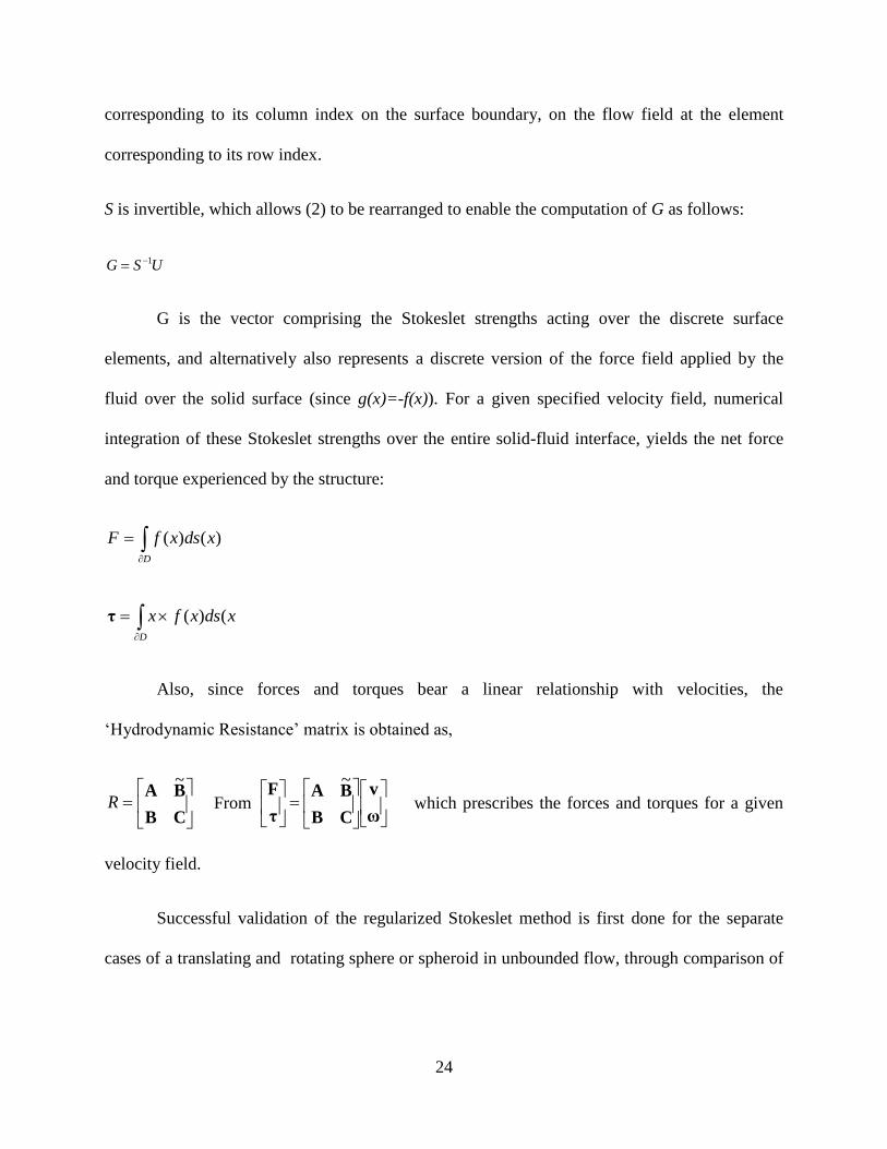
S is an assembled 3N x 3N matrix comprising of 3x3 sub-matrix units, each of which

being a Stokeslet tensor matrix, representing the effect of force strength at the discrete element

24

corresponding to its column index on the surface boundary, on the flow field at the element

corresponding to its row index.

S is invertible, which allows (2) to be rearranged to enable the computation of G as follows:

USG 1

G is the vector comprising the Stokeslet strengths acting over the discrete surface

elements, and alternatively also represents a discrete version of the force field applied by the

fluid over the solid surface (since g(x)=-f(x)). For a given specified velocity field, numerical

integration of these Stokeslet strengths over the entire solid-fluid interface, yields the net force

and torque experienced by the structure:

D

xdsxfF )()(

D

xdsxfx ()(τ

Also, since forces and torques bear a linear relationship with velocities, the

„Hydrodynamic Resistance‟ matrix is obtained as,

CB

BA~

R From

ω

v

CB

BA

τ

F~

which prescribes the forces and torques for a given

velocity field.

Successful validation of the regularized Stokeslet method is first done for the separate

cases of a translating and rotating sphere or spheroid in unbounded flow, through comparison of

25

the drag force and torque computed as above, with well known theoretical expressions (Stokes‟

law).

The corresponding grand Resistance matrix for the case of a sphere of radius 1m, which

is hydrodynamically interacting with water (viscosity μ= 10-3

Pa.s), is computed to be,

8495.180014.00023.0

0017.08495.180019.0

0022.00015.08495.18

A

0013.00011.00027.0

0006.00032.00008.0

0015.00017.00025.0

B

4610.250008.00018.0

0019.04610.250024.0

0025.00031.04610.25

C

It can be seen from the above matrix elements, that the total numerical errors (comprising

of regularization, discretization and round-off errors) are small enough to give adequately

accurate results.

The close proximity of the solid slide in the nanomotor experiments requires appropriate

consideration of wall effects in the analysis, which are modeled through implementation of the

image system of a Regularized Stokeslet, Stokeslet doublet and potential dipole formulated by

Ainley et al. [14]

335

2

3

3

)22

3

32

)22

2

)22

6

)(42(

2((

),(

RRR

h

RhR

RRR

R

hR

Rh

R

RRR

r

rrrrxS

ijji

ikiii

k

jk

jiijjiijε

ij

26

Chapter 4: Validation of the Method of Regularized Stokeslets

4.1. Validation of the Image system for single particle wall Hydrodynamic interactions

To verify the validity of the image system, we perform a check with a point force applied

on a grid point near the wall, demonstrating the decay of the velocity field as the point of

observation is made to approach the wall, and also confirming an expected gradual decay of

velocity field on the other side, as the point of observation is moved away into the unbounded

fluid.

Further, to ensure a rigorous validation, the image system is tested and validated for the

following particle/wall interaction cases: sphere translating parallel to the wall at different gap

sizes from the wall, sphere rotating about an axis perpendicular to the wall at different gap sizes,

prolate spheroid translating parallel to the wall at different gap sizes, prolate spheroid rotating

about an axis perpendicular to the wall at different gap-sizes.

First, the test cases sphere/spheroid are geometrically modeled by means of parametric

representations of the surfaces – one parameter ranging from one axial tip to the other and the

second parameter ranging over the circumference on the sphere/spheroid surface at every

discrete first parameter value. The mesh (N =2400 for sphere; N=2977 for prolate spheroid) is

generated with this parametric description and the regularized image-system is tested. The

validation is demonstrated by close agreement of the magnitudes of drag force and drag torque,

computed using the above method, with the Faxen‟s asymptotic relations [17] for microspheres

translating/rotating in presence of a single plane wall. Figure 4.1 shows variation of the drag

force on a sphere translating parallel to the wall as it is moved closer to the wall, as prescribed by

27

Faxen‟s analytical relations and compares it with the drag variation predicted by the Regularized

Stokeslet method.

Figure 4.1: Variation of drag force acting on sphere of radius 1 µm, translating parallel to wall with speed U=1

µm/s, with distance from wall below. The drag determined from Faxen‟s asymptotic expression for symmetrical

bodies is compared with that obtained from the method of Regularized Stokeslet

Figure 4.2: Variation of drag torque acting on sphere of radius 1 µm, rotating about axis normal to wall with angular

speed equal to 1 rad/s, with distance from wall below. The drag torque computed from Faxen‟s asymptotic

expression for symmetrical bodies, is compared with that obtained from the method of Regularized Stokeslet.

0 0.1 0.2 0.3 0.4 0.5 0.60.015

0.02

0.025

0.03

0.035

0.04

0.045

Distance from the wall (m))

Dra

g T

orq

ue

(x 1

0- 18

Nm

)

Drag torque using Faxen analytical relation

Drag torque using Regularised stokeslet image system

0 0.1 0.2 0.3 0.4 0.5 0.6 0.7 0.8 0.9 12.5

3

3.5

4

4.5

5

Distance from the wall (m)

Dra

g F

orc

e (

x 1

0- 1

4 N

)

Drag using Faxen analytical relations

Drag using Regularised stokeslet image system

28

Figure 4.2 shows similar comparison of drag torques corresponding to a rotating sphere

near wall. Figures 4.3 and 4.4 present comparison of drag forces on a prolate spheroid, specified

geometrically by major axis = 1.5 µm and minor axis = 0.71 µm, translating along and

perpendicular to its major axis, respectively.

Figure 4.3: Variation of drag force (log) acting on prolate spheroid of major axis = 1.5 µm, minor axis =0.71 µm,

translating parallel to wall along the major axis, with speed equal to 1 µm/s , with variation of separation distance

from wall (log) starting far off. The drag determined from Faxen‟s asymptotic expression applicable for symmetrical

bodies, is compared with that obtained from the method of Regularized Stokeslet.

5.2 5.4 5.6 5.8 6 6.2 6.4 6.6 6.8 70.4935

0.494

0.4945

0.495

0.4955

0.496

0.4965

0.497

0.4975

(log) distance from wall (m) (major axis=1.5, minor axis= 1/sqrt(2))

(lo

g)

Dra

g F

orc

e (

x 1

0- 14

N)

Drag Force using Faxen analytical relation

Drag force using Regularised stokeslet image system

29

Figure 4.4: Variation of drag force (log) acting on prolate spheroid of major axis = 1.5 µm, minor axis =0.71 µm,

translating parallel to wall along the minor axis, with speed equal to 1 µm/s , as separation from wall (log)

decreases, starting from far off. The drag determined from Faxen‟s asymptotic expression applicable for

symmetrical bodies is compared with that obtained from the method of Regularized Stokeslet

In the case of large gaps, the accuracy of the method is high, and does not depend

strongly on the regularization parameter and grid size. On the other hand, in the near wall case,

the method is only highly accurate up till a minimum gap size, which, understandably, is a

function of both the grid size as well as the regularization parameter. However, the regularization

parameter, ε is typically chosen as the following power function of the grid size (

9.037.0 sizegridaverage

for sphere; 9.0

3.0 sizegridaverage for spheroid), and, it

is determined that appropriate choice of the grid size allows good accuracy down to a gap size

5.2 5.4 5.6 5.8 6 6.2 6.4 6.6 6.8 70.64

0.6405

0.641

0.6415

0.642

0.6425

0.643

0.6435

(log) distance from wall (m) (major axis=1.5, minor axis= 1/sqrt(2))

(lo

g)

Dra

g F

orc

e (

x 1

0- 14

N)

Drag Force using Faxen analytical relation

Drag force using Regularised stokeslet image system

30

equal to one-hundredth of the nanomotor radius. This permits use of the method even for

extremely small distances from the wall, without any appreciable loss in accuracy.

4.2. Validation of the Stokeslet system for pair Hydrodynamic interactions

To demonstrate the validity of the Stokeslet method in situations of hydrodynamic

interactions between multiple structures, we consider the case where one sphere s1 is moving in

a fluid in proximity to a second sphere s2 which is stationary. We aim to determine the effect of

this translating/rotating sphere on the nearby sphere by evaluating the force and torque

transmitted by the moving sphere to the stationary sphere through the flow-field. To represent

the corresponding hydrodynamic situation in terms of Stokeslets, we consider the force-field on

the flow generated by the moving sphere as a collection of individual point force-strengths

existing over a surface in the flow domain, evaluate its influence on the flow-field around the

nearby stationary sphere, and thereby, determine how it affects the dynamics of the nearby

sphere.

The implementation of the Stokeslet method for evaluation of hydrodynamic interaction

between multiple particles differs slightly from that of a single particle interacting with flow

around it. However, the same force strength-speed coupled relation following from the boundary

integral formulation, and the Green‟s function tensor, enables the description of particle-particle

hydrodynamic interactions starting from the fundamental force-field relations in Stokes flow as

outlined below.

31

)3(,8

1

1

3

1

,00

N

n i

iinnijj AgxxSxu

0xu j , is the velocity vector at location x0 in the flow field, and here including points on the

surfaces of each of the two particles

The following Stokes flow Green‟s functions (Stokeslet), would represent the

hydrodynamic coupling between the force field and the flow-field for all points over both the

moving sphere and the stationary sphere, and employed in accordance to the investigation being

in unbounded flow domain or in presence of no-slip wall

)(2

,2/322

,0,0

2/322

22

0 flowunboundedr

xxxx

r

rxxS

jjii

ijij

The image-system of a Stokeslet, Stokeslet doublet and potential dipole formulated by Ainley et

al. is employed to account for wall effects [14]

)(6

)(42(

2((

),(

335

2

3

3

)22

3

32

)22

2

)22

wallslipnoofpresenceinRRR

h

RhR

RRR

R

hR

Rh

R

RRR

r

rrrrxS

ijji

ikiii

k

jk

jiijjiijε

ij

gn,i is the ith component of the point force-strength acting on the fluid at location xn and

aggregated to form the force-strength vector including the discrete strengths representing the

entire force-field on the flow.

We aim to evaluate the net hydrodynamic force induced by the force field generated by

the moving sphere s2, on the nearby stationary sphere s1, and thereby, determine how it affects

32

the dynamics of the nearby sphere. As mentioned before, the force-field on the flow generated by

the moving sphere is considered to be a collection of individual point force-strengths existing

over the surface boundary in the flow.

Eq. (3) translates to the linear system in the same way as shown for the single particle case:

22121 GSU

Here, S1-2 is the assembled matrix (3N x 3N) comprising of 3 x 3 Stokeslet tensor

matrices, representing the effect of point force-strengths around the moving sphere on velocity

induced in flow around the other stationary sphere, and G2 is the vector comprising of individual

force strengths acting on the flow around the moving sphere, the interaction induced velocity

vector, U1-2 is to be computed as a solution of the above linear system.

Owing to the coupled nature of hydrodynamic interactions between the two particles, the

stationary sphere in turn affects the dynamics of the moving sphere to be again represented by

the following linear system.

11212 GSU

S2-1, here, is the assembled matrix (3N x 3N) comprising of Stokeslet tensor matrices,

representing the effect of point force-strengths around the stationary sphere on velocity induced

in flow around the moving sphere, and G1 is the vector comprising of individual force strengths

acting on the flow around the stationary sphere, while the interaction induced velocity vector,

U2-1 is to be computed as solution of the above linear system.

33

In addition to the mutual hydrodynamic interaction formulated as above, the self

hydrodynamic relations, prescribing the effect of force strengths over a structure boundary, on

the flow-field over the same boundary, lead to the following linear systems.

)2(2222211111 GSUandGSU

S1-1 and S2-2, here, are the assembled Stokeslet tensor matrices, representing the effect of

point force-strengths around the stationary sphere and moving sphere respectively, on velocity

induced over their respective boundaries, and G1 and G2 again, are respectively the vectors

comprising of individual force strengths acting around the stationary and the moving sphere, the

self mobility velocity vectors, U1-1 and U2-2 would be computed as solutions of the above linear

systems.

It is clearly seen that the above hydrodynamic relationships are strongly coupled and the

hydrodynamic description of the entire system of sphere pairs need to be represented by

aggregating the above linear systems into a single linear system.

)4(. GSU

Here, S is the assembled matrix (6N x 6N), constructed from the abovementioned S1-1 S2-2, S1-

12and S2-1 matrices such that

2212

2111

SS

SSS

G again, is a force-strength vector representing the force-field existing over boundaries of both

the structures such that

34

2

1

G

GG

U then, is the velocity vector with 6N elements constructed by putting together 3N points over

the originally stationary sphere and another set of 3N points from the moving sphere such that

2

1

U

UU

S is invertible, which allows (4) to be rearranged to enable the computation of G as follows:

USG 1

For the purpose of validation, we employ the following vector U.

2

6

2

13

1

3

1

1

0

0

1

0

0

1

0

0

0

0

0

0

N

N

N

|

|

|

|

|

U

35

Numerical integration of these induced Stokeslet force-strengths over the surface

boundary of sphere s1, yields the net force and torque individually experienced by both spheres.

For the purpose of validation, we would consider the force and torque induced by the moving

sphere s2 on the originally motionless sphere s1

D

xdsxgF )()(121

D

xdsxgx )()(121τ

where g1‟s are the individual force strength elements making up the entire force-strength vector

acting on sphere s1, and also represent the induced force-strengths by the moving sphere on the

originally stationary sphere.

To start with, the test case sphere is geometrically modeled again, by means of the

previously used parametric representation of the surface – one parameter ranging from one axial

tip to the other and the second parameter ranging over the circumference on the sphere surface at

every discrete first parameter value. The mesh (N =2400 for sphere) is generated with this

parametric description and the regularized Stokeslet system for unbounded flow as well as the

regularized image system for single wall bounded flow, are tested. The validation is

demonstrated by comparison of magnitudes of the induced force and torque, computed first for

unbounded flow situation using the above method, with the analytical expressions by Happel and

Brenner for interaction between a pair of spheres in unbounded flow where one of the spheres is

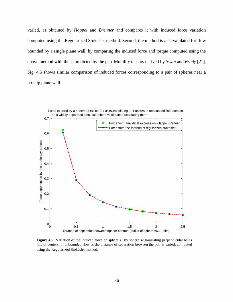
translating/rotating [10]. Fig. 4.5 shows variation of the induced force on sphere s1 by sphere s2

translating perpendicular to its line of centers, as the distance of separation between the pair is

36

varied, as obtained by Happel and Brenner and compares it with induced force variation

computed using the Regularized Stokeslet method. Second, the method is also validated for flow

bounded by a single plane wall, by comparing the induced force and torque computed using the

above method with those predicted by the pair-Mobility tensors derived by Swan and Brady [21].

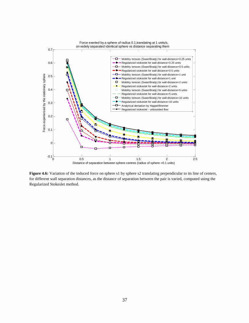
Fig. 4.6 shows similar comparison of induced forces corresponding to a pair of spheres near a

no-slip plane wall.

Figure 4.5: Variation of the induced force on sphere s1 by sphere s2 translating perpendicular to its

line of centers, in unbounded flow as the distance of separation between the pair is varied, computed

using the Regularized Stokeslet method.

0 0.5 1 1.5 2 2.50

0.1

0.2

0.3

0.4

0.5

0.6

0.7

Force exerted by a sphere of radius 0.1 units,translating at 1 units/s in unbounded fluid domain,

on a widely separated identical sphere vs distance separating them

Distance of separation between sphere centres (radius of sphere =0.1 units)

Forc

e e

xperienced b

y t

he s

tationary

sphere

Force from analytical expression -Happel/Brenner

Force from the method of regularized stokeslet

37

Figure 4.6: Variation of the induced force on sphere s1 by sphere s2 translating perpendicular to its line of centers,

for different wall separation distances, as the distance of separation between the pair is varied, computed using the

Regularized Stokeslet method.

0 0.5 1 1.5 2 2.5-0.1

0

0.1

0.2

0.3

0.4

0.5

0.6

0.7

Force exerted by a sphere of radius 0.1,translating at 1 units/s, on widely separated identical sphere vs distance separating them

Distance of separation between sphere centres (radius of sphere =0.1 units)

Forc

e e

xperienced b

y the s

tatio

nary

sphere

Mobility tensors (Swan/Brady) for wall-distance=0.25 units

Regularized stokeslet for wall-distance=0.25 units

Mobility tensors (Swan/Brady) for wall-distance=0.5 units

Regularized stokeslet for wall-distance=0.5 units

Mobility tensors (Swan/Brady) for wall-distance=1 unit

Regularized stokeslet for wall-distance=1 unit

Mobility tensors (Swan/Brady) for wall-distance=2 units

Regularized stokeslet for wall-distance=2 units

Mobility tensors (Swan/Brady) for wall-distance=5 units

Regularized stokeslet for wall-distance=5 units

Mobility tensors (Swan/Brady) for wall-distance=10 units

Regularized stokeslet for wall-distance=10 units

Analytical derivation by Happel/Brenner

Regularized stokeslet - unbounded flow

38

Chapter 5: Mesh Generation

Accurate geometric modeling of the complete nanomotor is immensely critical for the

accuracy of the simulated results owing to the fact that the structure dynamics, which we are

computing using the Stokeslet method, are highly sensitive to the surface geometry and profile.

The silica spherical bead is modeled as a sphere of 1 µm radius. The arm described above to be

analogous to a thick fan blade, is modeled as an appropriately dimensioned ellipsoid (rather than

simply a cylinder or spheroid), in view of the importance of accurate geometric modeling and

since an ellipsoid offers more degrees of freedom facilitating accurate model fit. The thickness

(0.5 µm ) is chosen as the smallest axis, increasing blade-width (varying from 1.6 µm to 1.8 µm

) as the next greater axis, and the length of the arm (0.86 µm, 1.25 µm, 1.75 µm, 2.5 µm, 3 µm)

as the greatest axis. The mesh is generated over the structure-surface with its parametric

description, in a way such that the average grid size is consistent all over the surface despite

different parameterization for the sphere bead and ellipsoidal arm.

The general ellipsoid is a quadratic surface, described in Cartesian coordinates by

12

2

2

2

2

2

c

z

b

y

a

x

where the semi-axes are of lengths a , b and c . If the lengths of two axes of an ellipsoid are the

same, the figure becomes a spheroid (an oblate spheroid or prolate spheroid, depending on

whether ac or ac respectively), and if all three are the same, it is a sphere. Alternately, it

can also be described parametrically as

39

sinsin

sincos

cos

cz

by

ax

where 20 and 0

We can set cba to represent a sphere by the above parametric description, and

model the spherical silica bead with it.

It is the aforementioned parametric description which is used to generate the mesh over

the surface of the structure, separately describing the spherical bead portion and the fan blade

like arm portion. The discrete grid elements are generated by prescribing their respective grid

points, in accordance to the above parameterization and then discretizing the parameters and

for the range appropriate to its arm size.

For generating the grid points of the sphere mesh, the parameters and are varied over

their full range to encompass the entire spherical surface except for the portion enveloped by its

joint with the arm, which in turn is left out by looking at the condition of its intersection with the

ellipsoid, specified to represent the arm. The following are the specifications for the sphere mesh

mcba 1

For generating the grid points on the arm, the parametric equations need to be

appropriately modified to account for the 90ο rotated orientation of the ellipsoid with respect to

its conventional configuration and the modified form is

40

cos

sinsin

sincos

bz

cy

ax

Also, here

ma 27.8 , length of semi axis along the length of the arm

mb 80.1 , length of semi axis along the width of the arm, analogous to fan-blade width

mc 25.0 , length of semi axis along the thickness of the arm

The parameter takes the value 180

125at the upper joint of the arm with the spherical

bead, and 180

235at the lower joint. The parameters for ellipsoid i.e. a , b and c are designed to

cause the axial length between its end sections (ellipsoid midsection representing arm free end)

to come out equal to m50.3 , as ranges from the aforementioned values at the joint, to values

of 2

and

2

3at the arm free end. We cut out sections from the free end (corresponding to

2

and 2

3 ), to obtain arms of different specified lengths (0.86 µm, 1.25 µm, 1.75 µm, 2.5 µm,

3 µm)

Table 2 lists the mesh description with discretization parameters for the nanomotor

structure of different arm-lengths

41

Table 2: Mesh description with discretization parameters for the nanomotor structure of different arm-lengths

In order to put the spherical and ellipsoidal geometric models together, such that the

combination correctly represents the actual structure, the ellipsoid arm needs to undergo an

inversion prior to attachment with the sphere bead, followed by a translational transformation to

position its end over the spherical bead surface.

Further, the arm inclination (here 45ο), is realized by means of rotation of the ellipsoid

about the central point of its surface of intersection with the sphere bead, which is brought about

by multiplying the following rotation transformation matrix with the position vector of the

structure. θ, here denotes the angle of inclination.

Arml

ength

Spherical Silica Bead

Ellipsoidal TiO2 Arm

Elliptical End Surface

Grid

Points

Surface

Size(µm2

)

Mean

Grid

Size(µ

m2)

Grid

Points

Surface

Size(µm2

)

Mean

Grid

Size(

µm2)

Grid

Points

Surface

Size(µm2

)

Mean

Grid

Size(

µm2)

.86

µm

1096 11.83 1.08e-

02

628 6.71 1.07e-

02

100 1.07 1.07e

-02

1.75

µm

1096 11.83 1.08e-

02

1587 17.18 1.08e-

02

100 1.07 1.07e

-02

2.50

µm

1096 11.83 1.08e-

02

2315 24.94 1.08e-

02

100 1.07 1.07e

-02

3.00

µm

1096 11.83 1.08e-

02

2675 28.89 1.08e-

02

100 1.07 1.07e

-02

3.50

µm

1096 11.83 1.08e-

02

2754 29.41 1.07e-

02

100 1.07 1.07e

-02

42

cossin

sincos

Figure 5.1 shows typical nanomotor geometry used in the simulations, corresponding to

an arm length of 3.5 µm (axes labels are in microns). The figure also shows the mesh used in the

implemented regularized Stokeslet algorithm, and is obtained by the parameterization technique

described above.

Figure 5.1: Typical nanomotor geometry used in the simulations, corresponding to an arm length of 3.5 µm (axes

labels are in microns). A nanomotor is modeled as a sphere connected to a section of an ellipsoid representing the

arm. Sections of different lengths are removed from the free end of the ellipsoid to match experimental conditions.

The figure also shows the mesh used in the regularized Stokeslet algorithm, which was obtained by parameterization

of the sphere and ellipsoid surfaces.

43

(a)

(b)

Figure 5.2: (a) Mesh generated for nanomotor of armlength

1.7μm; (b) Modeled structure geometry for the same

(a)

(b)

Figure 5.3: (a) Mesh generated for nanomotor of armlength

3.5 μm; (b) Modeled structure geometry for the same

44

Straightforward specification of the range of parameters for the ellipsoid arm, to describe

the arm surface geometry, results in wide variation in grid sizes spread over the surface profile,

such that, the grid lines become more dense close to the central axis along the length of the arm,

and relatively sparse elsewhere. Owing to this, convergence is not strictly observed with

increasing grid refinement, as the Stokeslet strength becomes nearly singular because of inter-

grid point spacing present in the denominator of its expression. Appropriate shift in parameter

range specification resolves this issue by leading to more uniform grid sizes over the surface

geometry and helps to ensure convergence.

45

Chapter 6: Nanomotor Dynamics - Modeling and Simulation

6.1. Modeling

Because a portion of spherical bead surface is enveloped by the joint with the arm, the

propulsion force resulting from the Pt-H2O2 reaction, is not aligned with the central axis of

symmetry, and hence the propulsion force field cannot be conveniently modeled as a single

resultant point force, applied symmetrically along the axis of the Pt coated hemisphere.

Consequently, the force field is appropriately modeled as a force distribution, which is

vectorially summed up over the exposed portion of the catalytic coating on the hemisphere. The

moment of the propulsion force is computed as the sum of the individual moments due to

discrete force strengths approximating the continuous force-field. In order to determine the

motion characteristics with variation in armlengths from our simulation scheme, corresponding

to the H2O2 solution under which the motion was studied experimentally (10% in this case), it is

essential to estimate the associated force-field strength to run the simulations. To estimate the

magnitude of this force strength corresponding to 10%, H2O2 solution, we record the motion of

the same structure with same Pt coating, but without any arm, when placed in 10% H2O2

solution. The observed translational speed leads to the determination of the drag force on the

structure by conferring with Faxen‟s analytical expressions [10] for hydrodynamic drag, well

known for simple symmetrical structures like spheres. In Stokes flow, this drag experienced

would settle down to equalize the catalytic propulsion force, thereby allowing us to determine

the propulsion force.

46

The grand „Hydrodynamic Resistance‟ matrix, R , for the precisely modeled nanomotor

geometry, is obtained using the following relationship, which stipulates the force/torques

experienced by the structure in response to its motion in the solution

CB

BA~

R from

ω

v

CB

BA

τ

F~

To determine the motion characteristics of the nanomotor, modeled geometrically and

dynamically in accordance to the aforementioned description, the „Mobility Matrix‟ of the

nanomotor is computed first, by inverting the „Resistance Matrix‟:

1~

CB

BAM which stipulates the velocities as:

6.2. Simulation

The velocities thus computed are utilized to simulate the motion of nanomotor, by

calculating its trajectory using a time marching scheme.

τ

F

CB

BA

ω

v1~

47

A natural value to calculate in order to characterize the trajectory curves, is the curvature,

)(t , which gives a quantitative value for how much the trajectory is changing direction. Our

simulation returns a list of the x and y coordinates of the particle, which describes its motion over

a certain time interval in accordance to its v and , determined as illustrated above.

This discrete set of x-y coordinates is fit with a circular path whose radius gives an

estimate of the average curvature of the actual irregular orbital trajectories. The following

method is used to determine the mean radius of curvature of the trajectories: the trajectories are

divided into nearly circular sections, that are fit with a circular path of equation

222 )()( rbyax whose radius r gives an estimate of the average radius of curvature of

the section. Following Kása, [22] this is achieved by minimizing the sum of the squares of the

distances from the discrete points ),(.......),,(),,( 2211 nn yxyxyx on the trajectory section to points

on the circle. Specifically, the following function is minimized over the unknown parameters a,

b, and r:

n

i

ii byaxrrbaSSK1

2222 )()(),,(

Kása further points out that solution for a and b can be obtained by solving linear

equations, and the radius of curvature is then obtained as:

n

i

ii nbyaxr1

22 /)()(

and averaged over all the trajectory sections. Finally, the mean trajectory curvature κ is

determined as the inverse of the average radius of curvature obtained above.

48

Chapter 7: Simulation Results

The preliminary simulations did predict sweeping orbital motions, resembling trajectories

seen experimentally, however our simulations predicted constant curvature magnitudes, which

were unchanging corresponding to different orbital speeds . Owing to the linear relationship

existing between the propelling force magnitude and the torque resulting from it, increasing the

intensity of propelling force by raising H2O2 concentration levels, and running the simulations,

predicts increase in both v and ω by the same factor, and thus, no change in curvatures.

Experiments, on the other hand, exhibit steadily increasing trend in the curvature with such

increase in orbital speeds. Careful consideration of the physical situation, suggested a possible

explanation for such change in the curvature with variation in propulsion force, in the form of a

likely presence of dynamic effects owing to structure-substrate solid friction. Observations

indicate contact between structure and glass-slide below and thereby, suggest presence of solid-

friction. We find that including a solid-frictional force and torque from the substrate, as

prescribed by an established velocity dependent friction model at micro/nanoscale friction [19],

does reproduce the trends seen in experiments, and justifies our hypothesis of structure-substrate

contact. The details of the appropriate friction model employed, are included in Appendix C.

The contact of the structure with the substrate under it is considered to be a point contact

coinciding with the central point of the spherical bead, while the arm portion of the structure,

based on its geometry, is reasonably assumed to be off the substrate. Accordingly, the friction

force is made to act at the sphere bead contact point, and the torque about the center of mass of

the overall structure arising out of this is duly taken into account to represent the influence of this

solid-friction on the structure dynamics.

49

Figure 7.1: Simulated nanomotor trajectories, for different arm lengths. Axes labels are in microns. In the absence

of Brownian motion, closed regular circular trajectories are obtained, with a radius of curvature that decreases with

increasing arm length.

Simulated particle trajectories for different arm lengths, without accounting for the

Brownian fluctuations, are shown in Fig. 7.1, and can be compared to Fig. 2.2 from the

experiments. These initially simulated trajectories, found to be closed circles with constant

curvature, differed from the more irregular trajectories of Fig. 2.2, seemingly due to the presence

of thermal fluctuations (Brownian motion) in the experiments, which were not accounted for in

the initial model. Again, good quantitative agreement was obtained for long arm lengths, but

slight discrepancies were present in the case of short arm lengths; which may be attributed to

Brownian fluctuations being more significant in the case of shorter arms. Similar trends were

observed for the curvature vs. speed, where we again found that good agreement was obtained at

high speeds, while the behavior at low speeds was not captured as accurately by the simulations,

50

owing to the increased importance of Brownian motion. It could be easily appreciated that an

appropriate consideration of Brownian effects in the model, would lead to improved

correspondence with the experimental observation, across all orbital speeds.

Hence, the Brownian fluctuations are precisely modeled as the stochastic solution to a

Langevin Equation, based on a random-walk model [19]. The simulations then give rise to

irregular trajectories showing better agreement with the observed trajectories as depicted in

Fig.7.2

Figure 7.2: Simulated nanomotor trajectories, for different arm lengths. Axes labels are in microns. In the presence

of Brownian dynamics, closed nearly circular trajectories are obtained which are not as smooth, with a radius of

curvature that decreases with increasing arm length.

-15 -10 -5 0 5 10 15-15

-10

-5

0

5

10

15

x (m)

y (

m)

R=8.31029

R=4.61396

R=2.3882

R=2.052

0.86 m

1.7 m

2.5 m

3 m

51

An animated simulation of nanomotor trajectories, for different arm lengths, is discussed in

Appendix D and is supplemented as a video file with the pdf version of the thesis.

In this way, Brownian fluctuations and micro/nanoscale surface related friction are

precisely included to take these additional effects into account. Appendices B and C, describe the

details of the models used for both.

The mobility relationship between force/torque and velocity/angular speed, after

incorporation of solid friction force/torque and Brownian force/torque vectors, may then be

expanded as

The new simulation results then show much better agreement with the curvature-speed

trends observed experimentally (Fig. 7.4), and for the low speed regime in particular, where

previously the discounting of Brownian forces failed to explain the higher than predicted

curvature values as can be seen in Fig. 7.3.

The experimental observations show increase in curvature with increasing arm length

which is shown more quantitatively in Fig. 7.5 where the curvature and angular frequency of the

nanomotors in the simulations is compared to the experimental data. Prior to the inclusion of

Brownian fluctuations, good quantitative agreement was still obtained for long arm lengths, but

discrepancies were present in the case of short arm lengths; attributed to Brownian fluctuations,

which are more significant in the case of shorter arms. After accounting for the Brownian forces

frictionbrownianhydτ

F

τ

F

τ

F

CB

BA

ω

v1~

52

and appropriate friction dynamics, the simulated results display very good quantitative

agreement even for short arm lengths as can be clearly seen in Fig. 7.5

0 1 2 3 4 5 6 7 8 9 100.10

0.15

0.20

0.25

0.30

0.35

0.40

0.45

0.50

0.55

0.60

Cu

rva

ture

(

m-1

)

Speed v (ms-1)

Figure 7.3.: For the OAD sample, there is observed a roughly linear increase of curvature with respect to speed. The

speed is increased by increasing the concentration of H2O2. The best-fit line gives a slope of 2104.6 s/μm2 .

Similar trends were determined from preliminary simulation without accounting for Brownian fluctuations , for the

curvature vs. speed, where we find that good agreement was obtained at high speeds, while the behavior at low

speeds was not captured as accurately by the simulations owing to the importance of Brownian motion not taken

into account. Moreover, nanoscale surface effects affecting solid friction also not considered, hence friction

characteristics included here did not fully represent the actual surface friction.

Figure 7.4: The Brownian fluctuations are appropriately modeled and the micro/nanoscale surface related velocity

dependent friction characteristics taken into account. The new simulation results show much better agreement with

the curvature-speed trends experimentally observed, and for the low speed regime in particular, where previously the

discounting of Brownian forces failed to explain the higher than predicted curvature values.

1 2 3 4 5 6 7 8 9

0.1

0.2

0.3

0.4

0.5

0.6

Cu

rva

ture

(

m-1

)

Speed v (ms-1)

Experiment

Simulation

53

Figure 7.5: The curvature and angular frequency of the nanomotors in the simulations is compared to the

experimental data. After accounting for the Brownian forces and appropriate friction dynamics, the simulated results

display very good quantitative agreement even for short arm lengths

-0.5 0.0 0.5 1.0 1.5 2.0 2.5 3.0 3.5 4.0

0.0

0.1

0.2

0.3

0.4

0.5

0.6

Cu

rva

ture

(m

-1)

Arm Length (m)

Experiment

Simulation

-0.5 0.0 0.5 1.0 1.5 2.0 2.5 3.0 3.5 4.0

0.0

0.5

1.0

1.5

2.0

2.5

3.0

3.5

An

gula

r F

requency

(

s-1)

Arm Length (m)

Experiment

Simulation

(a

)

(b

)

54

Chapter 8: Conclusion

The motion exhibited by catalytic Nanomotors in H2O2 solution, designed using the

dynamic fabrication methods OAD and GLAD, was experimentally studied by Gibbs and Zhao

[8]. It was observed that these structures display circular motion, such that the radii of curvature

decreases as the arm-lengths increases. It was also seen that increasing the concentration of H2O2

increases the speed of the structures and at the same time, the OAD nanomotor exhibits

trajectories of monotonically decreasing radii of curvature. We aimed, herein, to explain the

above observations by means of computational modeling and simulation and to predict the

structure dynamics as a function of its geometrical and environmental description.

We performed simulations that included an accurate representation of the nanomotor

geometry, full hydrodynamic interactions between components of the nanomotor and with the

supporting substrate, frictional forces with the substrate, as well as Brownian forces influencing

the motion.

The preliminary simulations, which discounted both the surface-contact effects and the

thermal fluctuations, did predict sweeping orbital motions, resembling observations made during

experimental investigation, however with unchanging curvature magnitudes, for the

corresponding orbital speeds. These initially simulated trajectories also differed from the more

irregular trajectories, seemingly due to the presence of thermal fluctuations (Brownian motion)

in the experiments, which were not accounted for in this initial model.

Moreover, owing to the linear relationship existing between the propelling force

magnitude and the torque resulting from it, increasing the intensity of propelling force by raising

55

H2O2 concentration levels, and running the simulations, predicted increase in both v and ω by

the same factor, and thus, implied no change in curvature. Experimental investigation, on the

other hand, depicted a steadily increasing trend in the curvature with corresponding increase in

orbital speed.

Careful consideration of the physical situation suggested a possible explanation for such

change in the curvature with propulsion force, in the form of a likely presence of dynamic effects

owing to structure-substrate solid friction. We found that including a solid-frictional force and

torque from the substrate, as prescribed by an established velocity dependent friction model for

micro and nanoscales [17], as well as precise modeling of Brownian fluctuations following from

the Langevin equation did reproduce the trends seen in experiments very well. The simulations

after inclusion of Brownian fluctuations then gave rise to irregular trajectories having better

qualitative agreement with the observed trajectories.

However, the presence of a degree of disagreement between the observed trajectories and

the simulated trajectories may be attributed to the idealized configuration adopted in the

simulations, in which the nanomotor arm was assumed to remain parallel to the supporting

substrate, as well as limitations in representatively modeling actual surface contact effects. Our

study also demonstrates that as the field of catalytic nanomotors matures, scientists and engineers

should consider the influence of nanomotor shape and geometry upon swimming behavior in

order to design better structures in the future.

56

References

[1] Paxton, W. F.; Sen, A.; Mallouk, T. E. “Motility of catalytic nanoparticles through self-generated forces,”

Chem.-Eur. J. 2005, 11, 6462.

[2] Gibbs, J. G.; Zhao, Y.-P. “Design and characterization of rotational multicomponent catalytic nanomotors,”

Small 2009, 5, 2304.

[3] Ebbens, S. J.; Howse, J. R. “In pursuit of propulsion at the nanoscale,” Soft Matter 2010, 6, 726.

[4] Fournier-Bidoz., S.; Arsenault, A. C.; Manners, I.; Ozin, G. A. Chem. Commun. Cambridge 2005, 4, 441.

[5] Qin, L.; Banholzer, M. J.; Xu, X.; Huang, L.; Mirkin, C. A. J. Am.Chem. Soc. 2007, 129, 14870.

[6] Soong, R. K.; Backand, G. D. ; Neves, H. P.; Olkhovets, A. G.; Craighead, H. G.; Montemango, C. D. Science

2000, 290, 1555.

[7] Ozin G. A.; Manners, I.; Fournier-Bidoz, S.; Arsenault, A. Adv. Mater.,Weinheim, Ger. 2005, 17, 3011.

[8] Gibbs, J. G.; Kothari, S.; Saintillan, D.; Zhao, Y.-P. “Geometrically Designing the Kinematic Behavior of

Catalytic Nanomotors,” Nano Lett. 2011. (submitted)

[9] Gibbs, J. G.; Zhao, Y.-P. Appl. Phys. Lett. 2009, 94, 163104.

[10] Happle, J.; Brenner, H., Low Reynolds Number Hydrodynamics. Prentice Hall: Englewood Cliffs, NJ, 1965.

[11] Kim, S.; Karrila, S. J., Microhydrodynamics: Principles and Selected Applications. Dover Publications, Inc.:

Mineola, NY, 2005.

[12] Cortez, R. SIAM J. Sci. Comput. 2001, 23, 1204.

[13] Pozrikidis, C. Boundary integral and singularity methods for linearized viscous flow; Cambridge University

Press: Cambridge, UK, 1992.

[14] Ainley, J.; Durkin, S.; Embid, R.; Boindala, P.; Cortez, R. J. Comp. Phys. 2008, 227, 4600.

57

[15] Smith, D. J. Proc. R. Soc. A 2009, 465, 3605.

[16] Blake, J. R. Proc. Camb. Phil. Soc. 1971, 70, 303.

[17] Leach, J.; Mushfique, H.; Keen, S.; Di Leonardo, R.; Ruocco, G.; Cooper, J. M.; Padgett M. J. Physical Review

E 79, 026301 2009

[18] Bhushan, B. Springer Handbook of Nanotechnology; Springer-Verlag: Berlin Heidelberg, Germany, 2nd

edn.

2007

[19] Liu H.; Bhushan B. Ultramicroscopy 91, 185–202 2002s

[20] Russel, W.B. “Brownian motion of small particles suspended in liquids,” Annu. Rev. Fluid Mech. 1981,

13, 425-455

[21] Swan, J. W.; Brady, J. F. “Simulation of hydrodynamically interacting particles near a no-slip boundary,” Phys.

Fluids 2007, 19, 113306.

[22] Kása, I. “A circle fitting procedure and its error analysis,” IEEE Trans. Instrum. Meas. vol. 25, pp. 8–14, Feb.

1976

[23] Tambe, N. S.; Bhushan B. Nanotechnology 16, 2309–2324 2005

[24] Chen, J.; Ratera, I.; Park, J. Y. and Salmeron, M. Phys. Rev. Lett. 96, 236102, 2006.

[25] Persson, B. Sliding Friction; Springer-Verlag: Berlin Heidelberg, Germany, 2nd

edn. 2000.

[26] Bowden, F.P.; Leben, L. “The nature of sliding and analysis of friction,” Proc. R. Soc. Lond. 1939, A 169, 371–

379.

[27] Gnecco, E.; Bennewitz, R.; Gyalog, T.; Loppacher, Ch; Bammerlin, M.; Meyer, E.; Guntherodt, H.J .”Velocity

dependence of atomic friction,‟ Phys. Rev. Lett. 2000, 84, 1172–1175.

[28] Riedo, E.; Gnecco, E.; Bennewitz, R.; Meyer, E.; Brune, H. “Interaction potential and hopping dynamics

governing sliding friction,” Phys. Rev. Lett. 2003, 91, 084502–1.

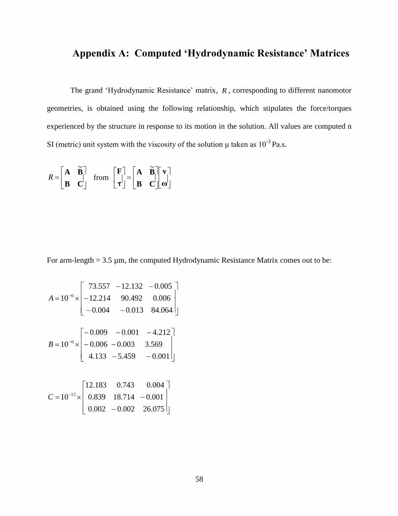
58

Appendix A: Computed ‘Hydrodynamic Resistance’ Matrices

The grand „Hydrodynamic Resistance‟ matrix, R , corresponding to different nanomotor

geometries, is obtained using the following relationship, which stipulates the force/torques

experienced by the structure in response to its motion in the solution. All values are computed n

SI (metric) unit system with the viscosity of the solution μ taken as 10-3

Pa.s.

CB

BA~

R from

ω

v

CB

BA

τ

F~

For arm-length = 3.5 µm, the computed Hydrodynamic Resistance Matrix comes out to be:

064.84013.0004.0

006.0492.90214.12

005.0132.12557.73

10 6A

001.0459.5133.4

569.3003.0006.0

212.4001.0009.0

10 6B

075.26002.0002.0

001.0714.18839.0

004.0743.0183.12

10 12C

59

For arm-length = 3 µm, the computed Hydrodynamic Resistance Matrix comes out to be:

011.78011.0005.0

002.0584.84135.10

002.0033.10639.70

10 6A

005.0383.4954.3

954.2002.0004.0

071.3005.0007.0

10 6B

314.21002.0003.0

004.0413.15583.0

003.0488.0781.9

10 12C

For arm-length = 2.5 µm, the computed Hydrodynamic Resistance Matrix comes out to be

011.78009.0005.0

003.0802.77048.9

002.0886.8321.64

10 6A

005.0418.3583.2

224.2001.0002.0

113.2003.0004.0

10 6B

110.16002.0004.0

003.0101.11302.0

001.0225.0323.7

10 12C

60

For arm-length = 1.7 µm, the computed Hydrodynamic Resistance Matrix comes out to be:

787.34007.0004.0

002.0608.64101.3

003.0920.2280.52

10 6A

003.0884.1311.1

643.5001.0002.0

832.4004.0002.0

10 6B

012.9001.0003.0

004.0491.6710.0

002.0351.0722.4

10 12C

For arm-length = 0.86 µm, the computed Hydrodynamic Resistance Matrix comes out to be:

128.39005.0003.0

002.0595.57734.1

001.0275.1512.48

10 6A

002.0354.4432.7

538.2001.0003.0

572.1002.0001.0

10 6B

242.4004.0001.0

003.0383.5402.0

006.0101.0281.4

10 12C

61

Appendix B: Brownian Fluctuation Modeling

The motion for a Brownian particle may be described by the Langevin equation as,

ebh FFFdt

dUm . (5)

which simply states that mass x acceleration equals the sum of the forces. In Eq. (5), m is a

generalized mass/moment of inertia matrix, of dimension 6x6, U is the particle

translational/rotational velocity vector of dimension 6, and the force/torque vectors on the right

hand side represent: (1) hF , the hydrodynamic force exerted on the particle due to its motion

relative to the fluid, (2) bF , the stochastic force that give rise to Brownian motion, and (3) eF ,

any other external force if applicable.

The stochastic or Brownian force bF arises from the thermal fluctuations in the fluid and

is modeled by:

0 bF and tkTRtFF bb 20

The angled brackets above denote an ensemble average, k is Boltzmann‟s constant, T is

the absolute temperature, R is the „Resistance‟ or the inverse Mobility of the particle and )(t is

the Dirac delta function. The amplitude of the correlation between the Brownian forces at time 0

and at time t results from the fluctuation-dissipation theorem [20].

62

The stochastic Brownian forces have zero mean and are correlated instantaneously in

time. The motion of the structure particle occurs on a time scalea

m

6

, which is long

compared to that of the fluid provided the particle size is large compared to that of a fluid

molecule. The amplitude of the correlation in the Brownian forces is chosen so that the mean

kinetic energy imparted to the particle is kT, where k is the Boltzmann constant and T is the

temperature in absolute scale, which forms the statement of the Equipartition theorem:

kTUmU2

1..

2

1 I

An evolution equation for the particle configuration is obtained by integrating Eq. (5)

twice over a time step t (larger than the inertial relaxation time, a

m

6

but small

compared with the time over which the configuration changes):

tFFFMx ebh

The Brownian force/torque as per the above Langevin description comes out as,

F

b Mt

kTF 2

12

Where F is a 3 element normal deviate vector, with expected value 0 and variance 1.

63

Here, the value of T is chosen to be 300K and the value of ∆t is chosen to be 10-6

seconds

which is larger than the inertial relaxation time, but smaller than the time over which there is a

perceptible change in the structure configuration.

Owing to an expectedly vital importance of Brownian forces on the system dynamics at

low propulsion force, suitable inclusion of the Brownian force, based on the random walk model,

gives simulated results which correspond quite well with the observed dynamics, especially for

the low velocity regime.

The consideration of Brownian force is also successful in representing the

characterization of observed dynamics for changing arm-lengths.

64

Appendix C: Contact Friction Modeling at Microscales

The increased importance of contact surface profile and surface related effects at

microscales, from the viewpoint of contact friction characterization, lead to the dependence of

the kinetic friction characteristics on the sliding and spinning speeds of the particle [18].

Based on the previously investigated velocity dependence of contact friction magnitude

[19], the friction is modeled accordingly and incorporated in the computational description. The

different postulated models are described below, of which, the Molecular Spring Model (4),

which is shown to be applicable for coated hydrophobic Si substrates in ethanol (similar to the

nanomotor Si substrate coated with Pt), is found to best represent the velocity dependence of

friction in our case.

Tambe and Bhushan [23] developed a comprehensive friction model starting from the

classical theory of friction by identifying the primary sources of nanoscale friction. The

nanoscale friction force between two contacting surfaces is essentially a result of three

components: interfacial adhesion between contacting asperities, energy required for deformation

of contacting asperities during relative motion, and stick-slip. The stick-slip effect can arise on

both atomic and micro/nanoscales and is known to be velocity-dependent. We may add all of

them to get the total friction force, F:

F=Fstick-slip + Fadh + Fdef

where

65

Fstick-slip = friction force due to atomic scale stick-slip between contacting surfaces,

Fadh = friction force due to adhesive interaction at the contacting surfaces,

Fdef = friction force due to deformation at the interface of the contacting surfaces.

1. Atomic Scale Stick-Slip Contribution to Friction Force

The term stick-slip, first coined by Bowden and Leben [26], corresponds to the build-up

of the friction force to a certain value, the static friction force, followed by slip at the interface

once this force is overcome.

Gnecco et al. [27] have derived an expression for the lateral force (friction force) based

upon the thermally activated jumps of the atoms in the proximity of an effective interaction

potential. Riedo et al. [28] showed that this increase continues up to a certain critical sliding

velocity vb and then levels off. Mathematically, the relation between the atomic scale stick-slip-

related friction force and the sliding velocity is given by:

21 ln cv

vcF

b

slipstick

where c1 and c2 are characteristic constants.

2. Adhesion Contribution to Friction Force

When two surfaces are placed in contact under a particular normal load, the contact takes

place at the asperity peaks, the load being supported by the deformation of the contacting

asperities, and discrete contact spots are formed. The proximity of the asperities results in

adhesive contacts caused by either physical or chemical interaction. When these surfaces move

66

relative to each other, a lateral force is required to shear the adhesive bonds formed at the

interface. This adhesive friction force, Fadh, for two contacting surfaces with a real area of

contact Ar and a relative sliding velocity v, is defined by

11 aradh AF

h

vA ar

11

where, α = fraction of dry contact (0 ≤ α ≤ 1), τa = average shear strength of dry contact, τl

average shear strength of liquid (water or lubricant) film, ηl =viscosity of liquid (water or

lubricant) film, h =thickness of liquid (water or lubricant) film.

The real area of contact is given by following equation:

2/1*

2/12.3

~p

pN

rE

RFA

Here FN = total normal load (normal load + meniscus forces, if any), E* = composite

Young‟s modulus for the two surfaces in contact, Rp =radius (average value) of asperity peaks,

σp= standard deviation of asperity peak heights.

For nanoscale contacts, the meniscus force contribution Fm may become comparable to

the normal load W and so the total normal load may also be written as

FN = W + Fm

67

3. Contribution of Asperity Deformation to Friction Force

This results from energy dissipation due to deformation of the contacting asperities.

During any relative motion, adhesion and asperity interactions are always present. Their

contribution, though, may or may not be significant, and this depends on surface roughness,

relative hardness of the two surfaces in contact, the normal load and sliding velocity. As the

relative sliding velocity increases, the impacts between surface asperities result in higher energy

dissipation. The deformation-related friction force can be written as

expended isenergy over which distance sliding

)dissipatedenergy frictional ( donework Fdef

If the normal load is small then the friction force due to deformation will become

dominant only at higher sliding velocities, when the energy from impacts is higher, and the

corresponding friction may be written as

Fdef = μdefW

where

z

kvN def

def

3/7

0

deformed asperities of numberasperity one deform toforce

68

3/2

2/1

*28

1

P

p

def

RE

m

R

Thus we see that the deformation-related friction force increases monotonically with sliding

velocity.

4. Molecular Spring Model

The velocity dependence of friction force for Si substrates with hydrophobic coating in

ethanol could not be explained using the analytical models described above. Liu and Bhushan

[19] have shown that there is an increase in friction force with velocity owing to reorientation of

asperities as predicted by the postulated Molecular Spring Model.

For a critical sliding distance sc, over which the molecules do not get sufficient time for

reorientation, we can determine the total friction force as

0104

FFs

sFF

c

, for s ≤ sc

where F0 and F1 are the maximum and minimum values of the friction force

The friction force can be expressed as a function of the ratio of the actual sliding velocity

v to the critical sliding velocity vc

69

vv

FFFF

c

4

010 , for v ≤ vc (6)

4

3 01 FFF , for v >vc

Liu and Bhushan’s data at high normal loads clearly shows a linear increase in friction

force followed by a distinct plateau beyond a certain critical velocity.

The linear relationship between the applied propulsion force and exhibited velocity is

used to represent (6) in terms of the applied propulsion force:

ff

FFFF

c

4

01

0

0

01

010 ff

ff

FFF

(7)

Here we use the following two characteristic force constants consistent in order of

magnitude with the physics of the problem:

F0= 0.001 pN, F1= 0.0018 pN,

f1 = 1.2 pN, f0=0.4 pN are estimates for the minimum and maximum values of the catalytic

propulsive force in the experiments.

70

Based on the above friction force characteristics, we may write the velocity dependent

frictional torque relation

0

01

01

0 ffff

TTF

(8)

where we use the following characteristic torque constants based on the aforementioned force

constants:

T0= 0.0000107 fNm, T1= 0.000025 fNm,

(7) and (8), thus, give the frictional force and torque magnitudes corresponding to the propulsion

force field known to be operating.

Using the above model relations, the results from simulations show good match with the

experimental data for velocity-curvature relation of the nanomotor. Similar friction

characteristics can also be verified from [24] and [25].

71

Appendix D: Animated Simulation of Nanomotor Trajectories

Animated simulation of nanomotor trajectories, for different arm lengths is

supplemented as a video file titled „Simulation_video.avi‟ ,with the electronic (pdf) version of

this thesis. Axes labels are in microns. It is observed that in the presence of Brownian dynamics,

the structures exhibit circular trajectories which are not as smooth, with a radius of curvature that

decreases with increasing arm length.