Embed Size (px)
Citation preview

© 2010 The McGraw-Hill Companies, Inc.
Standard Costs and Operating Performance Measures
Chapter 11

McGraw-Hill/Irwin Slide 2
Standard Costs
Standards are benchmarks or “norms” formeasuring performance. In managerial accounting,
two types of standards are commonly used.
Quantity standardsspecify how much of aninput should be used to
make a product orprovide a service.
Price standardsspecify how muchshould be paid foreach unit of the
input.
Examples: Firestone, Sears, McDonald’s, hospitals, construction and manufacturing companies.

McGraw-Hill/Irwin Slide 3
Standard Costs
DirectMaterial
Deviations from standards deemed significantare brought to the attention of management, apractice known as management by exception.
Type of Product Cost
Am
ou
nt
DirectLabor
ManufacturingOverhead
Standard
McGraw-Hill/Irwin Slide 4
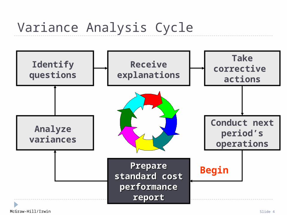
Variance Analysis Cycle
Prepare standard Prepare standard cost performance cost performance
reportreport
Analyze variances
Begin
Identifyquestions
Receive explanations
Takecorrective
actions
Conduct next period’s
operations

McGraw-Hill/Irwin Slide 5
Accountants, engineers, purchasingagents, and production managers
combine efforts to set standards that encourage efficient future operations.
Setting Standard Costs

McGraw-Hill/Irwin Slide 6
Setting Standard Costs
Should we useideal standards that require employees towork at 100 percent
peak efficiency?
Engineer Managerial Accountant
I recommend using practical standards that are currently
attainable with reasonable and efficient effort.

McGraw-Hill/Irwin Slide 7
Learning Objective 1
Explain how direct Explain how direct materials standards materials standards
and direct laborand direct laborstandards are set.standards are set.

McGraw-Hill/Irwin Slide 8
Setting Direct Material Standards
PriceStandards
Summarized in a Bill of Materials.
Final, deliveredcost of materials,net of discounts.
QuantityStandards
McGraw-Hill/Irwin Slide 9
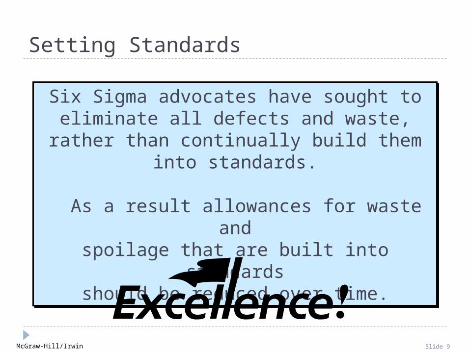
Setting Standards
Six Sigma advocates have sought toeliminate all defects and waste, rather than
continually build them into standards.
As a result allowances for waste andspoilage that are built into standards
should be reduced over time.
Six Sigma advocates have sought toeliminate all defects and waste, rather than
continually build them into standards.
As a result allowances for waste andspoilage that are built into standards
should be reduced over time.

McGraw-Hill/Irwin Slide 10
Setting Direct Labor Standards
RateStandards
Often a singlerate is used that reflectsthe mix of wages earned.
TimeStandards
Use time and motion studies for
each labor operation.

McGraw-Hill/Irwin Slide 11
Setting Variable Manufacturing Overhead Standards
RateStandards
The rate is the variable portion of the
predetermined overhead rate.
QuantityStandards
The quantity is the activity in the
allocation base for predetermined overhead.

McGraw-Hill/Irwin Slide 12
Standard Cost Card – Variable Production Cost
A standard cost card for one unit of product might look like this:
A A x BStandard Standard StandardQuantity Price Cost
Inputs or Hours or Rate per Unit
Direct materials 3.0 lbs. 4.00$ per lb. 12.00$ Direct labor 2.5 hours 14.00 per hour 35.00 Variable mfg. overhead 2.5 hours 3.00 per hour 7.50 Total standard unit cost 54.50$
B

McGraw-Hill/Irwin Slide 13
Price and Quantity Standards
Price and quantity standards are determined separately for two reasons:
The purchasing manager is responsible for raw material purchase prices and the production manager is responsible for the quantity of raw material used.
The purchasing manager is responsible for raw material purchase prices and the production manager is responsible for the quantity of raw material used.
The buying and using activities occur at different times. Raw material purchases may be held in inventory for a period of time before being used in production.
The buying and using activities occur at different times. Raw material purchases may be held in inventory for a period of time before being used in production.
McGraw-Hill/Irwin Slide 14
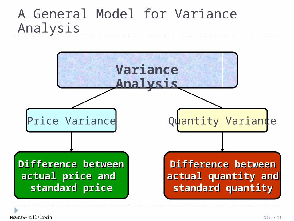
A General Model for Variance Analysis
Variance Analysis
Price Variance
Difference betweenDifference betweenactual price and actual price and standard pricestandard price
Quantity Variance
Difference betweenDifference betweenactual quantity andactual quantity andstandard quantitystandard quantity

McGraw-Hill/Irwin Slide 15
Variance Analysis
Materials price varianceLabor rate varianceVOH rate variance
Materials quantity varianceLabor efficiency varianceVOH efficiency variance
A General Model for Variance Analysis
Price Variance Quantity Variance

McGraw-Hill/Irwin Slide 16
Price Variance Quantity Variance
Actual Quantity Actual Quantity Standard Quantity × × × Actual Price Standard Price Standard Price
A General Model for Variance Analysis

McGraw-Hill/Irwin Slide 17
Price Variance Quantity Variance
Actual Quantity Actual Quantity Standard Quantity × × × Actual Price Standard Price Standard Price
A General Model for Variance Analysis
Actual quantity is the amount of direct materials, direct labor, and variable
manufacturing overhead actually used.

McGraw-Hill/Irwin Slide 18
Price Variance Quantity Variance
Actual Quantity Actual Quantity Standard Quantity × × × Actual Price Standard Price Standard Price
A General Model for Variance Analysis
Standard quantity is the standard quantity allowed for the actual output of the period.
McGraw-Hill/Irwin Slide 19
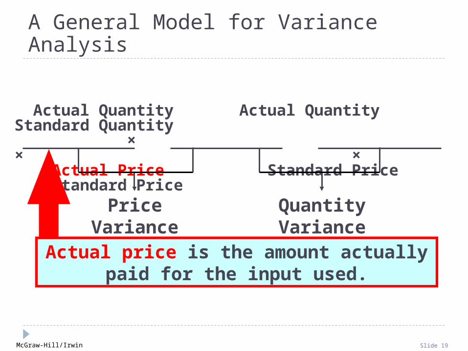
Price Variance Quantity Variance
Actual Quantity Actual Quantity Standard Quantity × × × Actual Price Standard Price Standard Price
A General Model for Variance Analysis
Actual price is the amount actuallypaid for the input used.

McGraw-Hill/Irwin Slide 20
A General Model for Variance Analysis
Standard price is the amount that should have been paid for the input used.
Price Variance Quantity Variance
Actual Quantity Actual Quantity Standard Quantity × × × Actual Price Standard Price Standard Price

McGraw-Hill/Irwin Slide 21
A General Model for Variance Analysis
(AQ × AP) – (AQ × SP) (AQ × SP) – (SQ × SP)
AQ = Actual Quantity SP = Standard Price AP = Actual Price SQ = Standard Quantity
Price Variance Quantity Variance
Actual Quantity Actual Quantity Standard Quantity × × × Actual Price Standard Price Standard Price

McGraw-Hill/Irwin Slide 22
Learning Objective 2
Compute the direct Compute the direct materials price and materials price and
quantity variances and quantity variances and explain their explain their significance.significance.

McGraw-Hill/Irwin Slide 23
Glacier Peak Outfitters has the following direct material standard for the fiberfill in its mountain
parka.
0.1 kg. of fiberfill per parka at $5.00 per kg.
Last month 210 kgs. of fiberfill were purchased and used to make 2,000 parkas. The material cost a
total of $1,029.
Material Variances – An Example

McGraw-Hill/Irwin Slide 24
210 kgs. 210 kgs. 200 kgs. × × × $4.90 per kg. $5.00 per kg. $5.00 per kg.
= $1,029 = $1,050 = $1,000
Price variance$21 favorable
Quantity variance$50 unfavorable
Actual Quantity Actual Quantity Standard Quantity × × × Actual Price Standard Price Standard Price
Material Variances Summary
McGraw-Hill/Irwin Slide 25
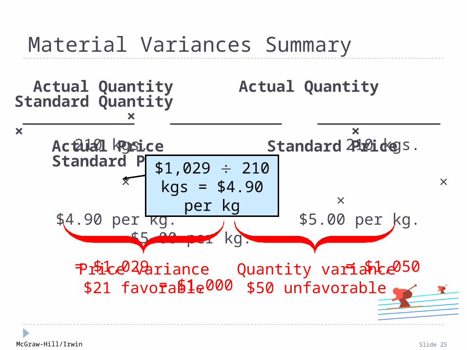
210 kgs. 210 kgs. 200 kgs. × × × $4.90 per kg. $5.00 per kg. $5.00 per kg.
= $1,029 = $1,050 = $1,000
Price variance$21 favorable
Quantity variance$50 unfavorable
Actual Quantity Actual Quantity Standard Quantity × × × Actual Price Standard Price Standard Price
$1,029 210 kgs = $4.90 per
kg
Material Variances Summary

McGraw-Hill/Irwin Slide 26
210 kgs. 210 kgs. 200 kgs. × × × $4.90 per kg. $5.00 per kg. $5.00 per kg.
= $1,029 = $1,050 = $1,000
Price variance$21 favorable
Quantity variance$50 unfavorable
Actual Quantity Actual Quantity Standard Quantity × × × Actual Price Standard Price Standard Price
0.1 kg per parka 2,000 parkas = 200 kgs
Material Variances Summary

McGraw-Hill/Irwin Slide 27
Material Variances:Using the Factored Equations
Materials price varianceMPV = AQ (AP - SP)
= 210 kgs ($4.90/kg - $5.00/kg)
= 210 kgs (-$0.10/kg)
= $21 F
Materials quantity varianceMQV = SP (AQ - SQ)
= $5.00/kg (210 kgs-(0.1 kg/parka 2,000 parkas))
= $5.00/kg (210 kgs - 200 kgs)
= $5.00/kg (10 kgs)
= $50 U

McGraw-Hill/Irwin Slide 28
Isolation of Material Variances
I need the price variancesooner so that I can better
identify purchasing problems.
You accountants just don’tunderstand the problems thatpurchasing managers have.
I’ll start computingthe price variancewhen material is
purchased rather than when it’s used.

McGraw-Hill/Irwin Slide 29
Material Variances
Hanson purchased and used 1,700 pounds.
How are the variances computed if the amount purchased differs from
the amount used?
The price variance is computed on the entire
quantity purchased.
The quantity variance is computed only on
the quantity used.
McGraw-Hill/Irwin Slide 30
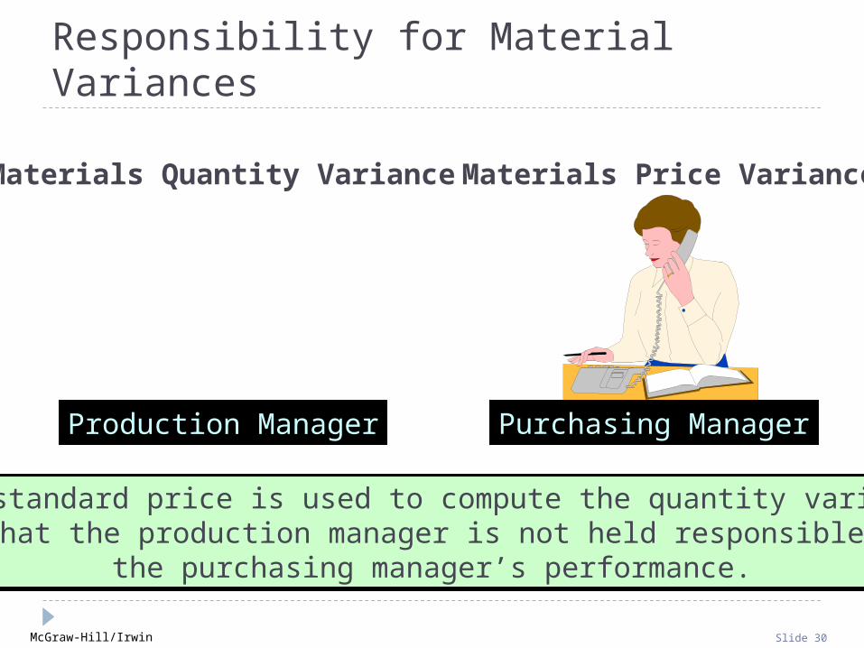
Materials Price VarianceMaterials Quantity Variance
Production Manager Purchasing Manager
The standard price is used to compute the quantity varianceso that the production manager is not held responsible for
the purchasing manager’s performance.
The standard price is used to compute the quantity varianceso that the production manager is not held responsible for
the purchasing manager’s performance.
Responsibility for Material Variances

McGraw-Hill/Irwin Slide 31
I am not responsible for this unfavorable material
quantity variance.
You purchased cheapmaterial, so my peoplehad to use more of it.
Your poor scheduling sometimes requires me to
rush order material at a higher price, causing
unfavorable price variances.
Responsibility for Material Variances

McGraw-Hill/Irwin Slide 32
Hanson Inc. has the following direct material standard to manufacture one Zippy:
1.5 pounds per Zippy at $4.00 per pound
Last week, 1,700 pounds of material were purchased and used to make 1,000 Zippies. The
material cost a total of $6,630.
ZippyQuick Check

McGraw-Hill/Irwin Slide 33
Quick Check Zippy
Hanson’s material price variance (MPV)for the week was:
a. $170 unfavorable.
b. $170 favorable.
c. $800 unfavorable.
d. $800 favorable.
Hanson’s material price variance (MPV)for the week was:
a. $170 unfavorable.
b. $170 favorable.
c. $800 unfavorable.
d. $800 favorable.

McGraw-Hill/Irwin Slide 34
Hanson’s material price variance (MPV)for the week was:
a. $170 unfavorable.
b. $170 favorable.
c. $800 unfavorable.
d. $800 favorable.
Hanson’s material price variance (MPV)for the week was:
a. $170 unfavorable.
b. $170 favorable.
c. $800 unfavorable.
d. $800 favorable. MPV = AQ(AP - SP) MPV = 1,700 lbs. × ($3.90 - 4.00) MPV = $170 Favorable
Quick Check Zippy

McGraw-Hill/Irwin Slide 35
Quick Check
Hanson’s material quantity variance (MQV)for the week was:
a. $170 unfavorable.
b. $170 favorable.
c. $800 unfavorable.
d. $800 favorable.
Hanson’s material quantity variance (MQV)for the week was:
a. $170 unfavorable.
b. $170 favorable.
c. $800 unfavorable.
d. $800 favorable.
Zippy

McGraw-Hill/Irwin Slide 36
Hanson’s material quantity variance (MQV)for the week was:
a. $170 unfavorable.
b. $170 favorable.
c. $800 unfavorable.
d. $800 favorable.
Hanson’s material quantity variance (MQV)for the week was:
a. $170 unfavorable.
b. $170 favorable.
c. $800 unfavorable.
d. $800 favorable. MQV = SP(AQ - SQ) MQV = $4.00(1,700 lbs - 1,500 lbs) MQV = $800 unfavorable
Quick Check Zippy

McGraw-Hill/Irwin Slide 37
1,700 lbs. 1,700 lbs. 1,500 lbs. × × × $3.90 per lb. $4.00 per lb. $4.00 per lb.
= $6,630 = $ 6,800 = $6,000
Price variance$170 favorable
Quantity variance$800 unfavorable
Actual Quantity Actual Quantity Standard Quantity × × × Actual Price Standard Price Standard Price
ZippyQuick Check

McGraw-Hill/Irwin Slide 38
Hanson Inc. has the following material standard to manufacture one Zippy:
1.5 pounds per Zippy at $4.00 per pound
Last week, 2,800 pounds of material were purchased at a total cost of $10,920, and 1,700
pounds were used to make 1,000 Zippies.
ZippyQuick Check Continued

McGraw-Hill/Irwin Slide 39
Actual Quantity Actual Quantity Purchased Purchased × × Actual Price Standard Price 2,800 lbs. 2,800 lbs. × × $3.90 per lb. $4.00 per lb.
= $10,920 = $11,200
Price variance$280 favorable
Price variance increases because quantity
purchased increases.
ZippyQuick Check Continued

McGraw-Hill/Irwin Slide 40
Actual Quantity Used Standard Quantity × × Standard Price Standard Price 1,700 lbs. 1,500 lbs. × × $4.00 per lb. $4.00 per lb.
= $6,800 = $6,000
Quantity variance$800 unfavorable
Quantity variance is unchanged because actual and standard
quantities are unchanged.
ZippyQuick Check Continued

McGraw-Hill/Irwin Slide 41
Learning Objective 3
Compute the direct Compute the direct labor rate and labor rate and
efficiency variances efficiency variances and explainand explain
their significance. their significance.

McGraw-Hill/Irwin Slide 42
Glacier Peak Outfitters has the following direct labor standard for its mountain parka.
1.2 standard hours per parka at $10.00 per hour
Last month, employees actually worked 2,500 hours at a total labor cost of $26,250 to make 2,000
parkas.
Labor Variances – An Example

McGraw-Hill/Irwin Slide 43
Rate variance$1,250 unfavorable
Efficiency variance$1,000 unfavorable
Actual Hours Actual Hours Standard Hours × × × Actual Rate Standard Rate Standard Rate
Labor Variances Summary
2,500 hours 2,500 hours 2,400 hours × × ×$10.50 per hour $10.00 per hour. $10.00 per hour
= $26,250 = $25,000 = $24,000

McGraw-Hill/Irwin Slide 44
Labor Variances Summary
2,500 hours 2,500 hours 2,400 hours × × ×$10.50 per hour $10.00 per hour. $10.00 per hour
= $26,250 = $25,000 = $24,000
Actual Hours Actual Hours Standard Hours × × × Actual Rate Standard Rate Standard Rate
$26,250 2,500 hours = $10.50 per hour
Rate variance$1,250 unfavorable
Efficiency variance$1,000 unfavorable

McGraw-Hill/Irwin Slide 45
Labor Variances Summary
2,500 hours 2,500 hours 2,400 hours × × ×$10.50 per hour $10.00 per hour. $10.00 per hour
= $26,250 = $25,000 = $24,000
Actual Hours Actual Hours Standard Hours × × × Actual Rate Standard Rate Standard Rate
1.2 hours per parka 2,000 parkas = 2,400 hours
Rate variance$1,250 unfavorable
Efficiency variance$1,000 unfavorable
McGraw-Hill/Irwin Slide 46
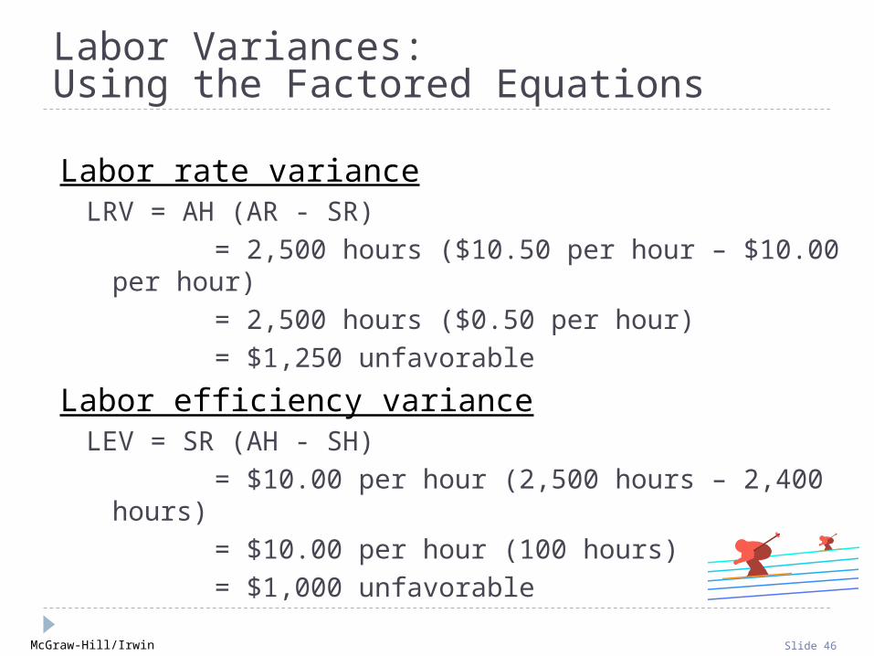
Labor Variances:Using the Factored Equations
Labor rate varianceLRV = AH (AR - SR)
= 2,500 hours ($10.50 per hour – $10.00 per hour)
= 2,500 hours ($0.50 per hour)
= $1,250 unfavorable
Labor efficiency varianceLEV = SR (AH - SH)
= $10.00 per hour (2,500 hours – 2,400 hours)
= $10.00 per hour (100 hours)
= $1,000 unfavorable

McGraw-Hill/Irwin Slide 47
Responsibility for Labor Variances
Production Manager
Production managers areusually held accountable
for labor variancesbecause they can
influence the:
Mix of skill levelsassigned to work tasks.
Level of employee motivation.
Quality of production supervision.
Quality of training provided to employees.

McGraw-Hill/Irwin Slide 48
I am not responsible for the unfavorable labor
efficiency variance!
You purchased cheapmaterial, so it took more
time to process it.
I think it took more time to process the
materials because the Maintenance
Department has poorly maintained your
equipment.
Responsibility for Labor Variances

McGraw-Hill/Irwin Slide 49
Hanson Inc. has the following direct laborstandard to manufacture one Zippy:
1.5 standard hours per Zippy at$12.00 per direct labor hour
Last week, 1,550 direct labor hours wereworked at a total labor cost of $18,910
to make 1,000 Zippies.
ZippyQuick Check

McGraw-Hill/Irwin Slide 50
Hanson’s labor rate variance (LRV) for the week was:
a. $310 unfavorable.
b. $310 favorable.
c. $300 unfavorable.
d. $300 favorable.
Hanson’s labor rate variance (LRV) for the week was:
a. $310 unfavorable.
b. $310 favorable.
c. $300 unfavorable.
d. $300 favorable.
Quick Check Zippy

McGraw-Hill/Irwin Slide 51
Hanson’s labor rate variance (LRV) for the week was:
a. $310 unfavorable.
b. $310 favorable.
c. $300 unfavorable.
d. $300 favorable.
Hanson’s labor rate variance (LRV) for the week was:
a. $310 unfavorable.
b. $310 favorable.
c. $300 unfavorable.
d. $300 favorable.
Quick Check
LRV = AH(AR - SR) LRV = 1,550 hrs($12.20 - $12.00) LRV = $310 unfavorable
Zippy

McGraw-Hill/Irwin Slide 52
Hanson’s labor efficiency variance (LEV)for the week was:
a. $590 unfavorable.
b. $590 favorable.
c. $600 unfavorable.
d. $600 favorable.
Hanson’s labor efficiency variance (LEV)for the week was:
a. $590 unfavorable.
b. $590 favorable.
c. $600 unfavorable.
d. $600 favorable.
Quick Check Zippy
McGraw-Hill/Irwin Slide 53
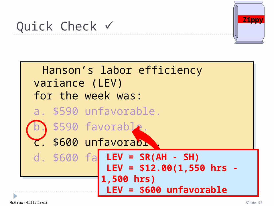
Hanson’s labor efficiency variance (LEV)for the week was:
a. $590 unfavorable.
b. $590 favorable.
c. $600 unfavorable.
d. $600 favorable.
Hanson’s labor efficiency variance (LEV)for the week was:
a. $590 unfavorable.
b. $590 favorable.
c. $600 unfavorable.
d. $600 favorable.
Quick Check
LEV = SR(AH - SH) LEV = $12.00(1,550 hrs - 1,500 hrs) LEV = $600 unfavorable
Zippy

McGraw-Hill/Irwin Slide 54
Actual Hours Actual Hours Standard Hours × × × Actual Rate Standard Rate Standard Rate
Rate variance$310 unfavorable
Efficiency variance$600 unfavorable
1,550 hours 1,550 hours 1,500 hours × × × $12.20 per hour $12.00 per hour $12.00 per hour
= $18,910 = $18,600 = $18,000
ZippyQuick Check

McGraw-Hill/Irwin Slide 55
Learning Objective 4
Compute the variable Compute the variable manufacturing manufacturing
overhead rate and overhead rate and efficiency variances.efficiency variances.

McGraw-Hill/Irwin Slide 56
Glacier Peak Outfitters has the following direct variable manufacturing overhead labor standard for its mountain
parka.
1.2 standard hours per parka at $4.00 per hour
Last month, employees actually worked 2,500 hours to make 2,000 parkas. Actual variable manufacturing
overhead for the month was $10,500.
Variable Manufacturing Overhead Variances – An Example

McGraw-Hill/Irwin Slide 57
2,500 hours 2,500 hours 2,400 hours × × × $4.20 per hour $4.00 per hour $4.00 per hour
= $10,500 = $10,000 = $9,600
Rate variance$500 unfavorable
Efficiency variance$400 unfavorable
Actual Hours Actual Hours Standard Hours × × × Actual Rate Standard Rate Standard Rate
Variable Manufacturing Overhead Variances Summary
McGraw-Hill/Irwin Slide 58
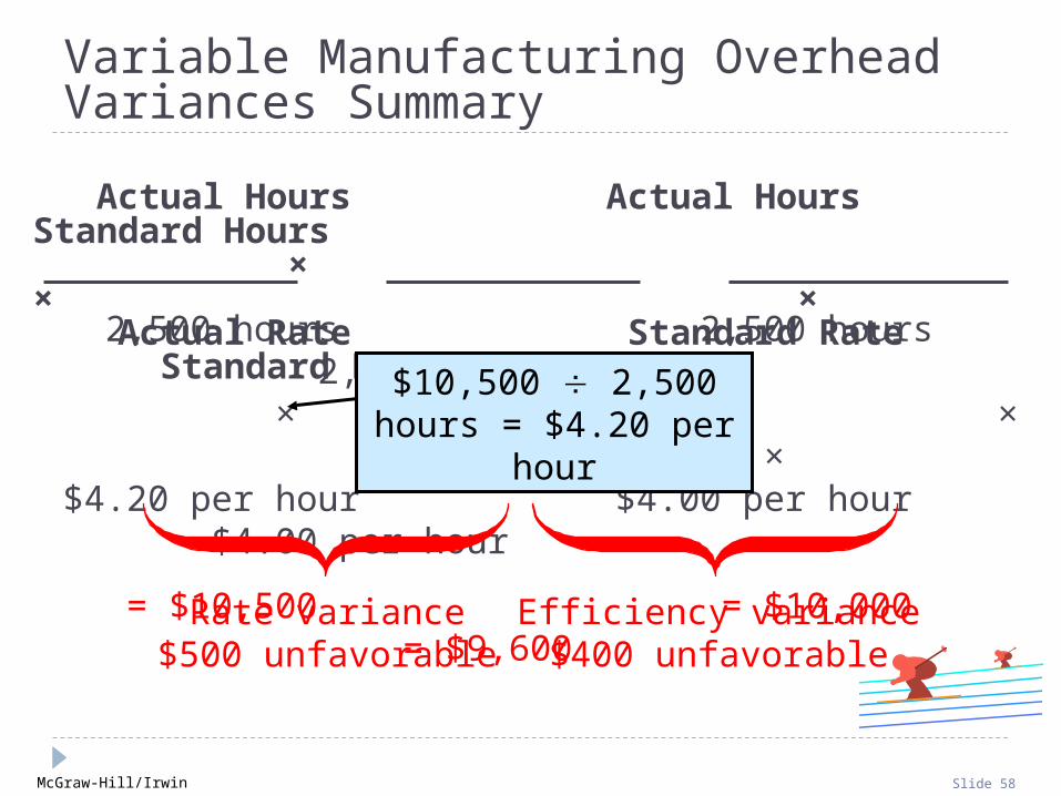
Actual Hours Actual Hours Standard Hours × × × Actual Rate Standard Rate Standard Rate
2,500 hours 2,500 hours 2,400 hours × × × $4.20 per hour $4.00 per hour $4.00 per hour
= $10,500 = $10,000 = $9,600
Rate variance$500 unfavorable
Efficiency variance$400 unfavorable
$10,500 2,500 hours = $4.20 per hour
Variable Manufacturing Overhead Variances Summary

McGraw-Hill/Irwin Slide 59
Actual Hours Actual Hours Standard Hours × × × Actual Rate Standard Rate Standard Rate
2,500 hours 2,500 hours 2,400 hours × × × $4.20 per hour $4.00 per hour $4.00 per hour
= $10,500 = $10,000 = $9,600
Rate variance$500 unfavorable
Efficiency variance$400 unfavorable
1.2 hours per parka 2,000 parkas = 2,400 hours
Variable Manufacturing Overhead Variances Summary

McGraw-Hill/Irwin Slide 60
Variable Manufacturing Overhead Variances: Using Factored Equations
Variable manufacturing overhead rate varianceVMRV = AH (AR - SR)
= 2,500 hours ($4.20 per hour – $4.00 per hour)
= 2,500 hours ($0.20 per hour)
= $500 unfavorable
Variable manufacturing overhead efficiency varianceVMEV = SR (AH - SH)
= $4.00 per hour (2,500 hours – 2,400 hours)
= $4.00 per hour (100 hours)
= $400 unfavorable
McGraw-Hill/Irwin Slide 61
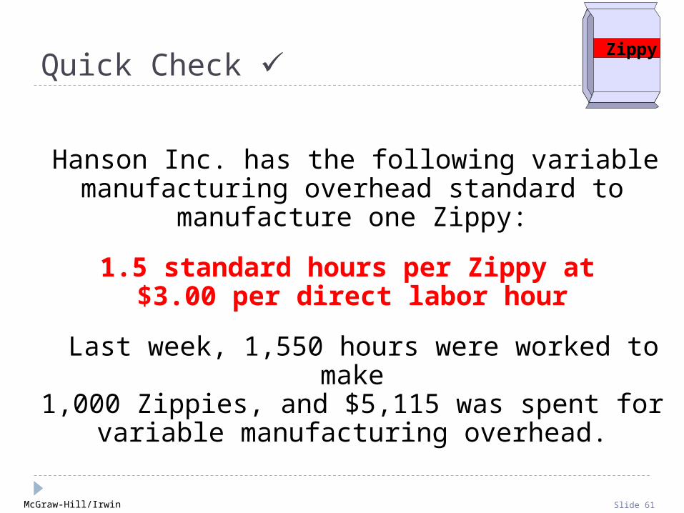
Hanson Inc. has the following variablemanufacturing overhead standard to
manufacture one Zippy:
1.5 standard hours per Zippy at$3.00 per direct labor hour
Last week, 1,550 hours were worked to make1,000 Zippies, and $5,115 was spent for
variable manufacturing overhead.
ZippyQuick Check

McGraw-Hill/Irwin Slide 62
Hanson’s rate variance (VMRV) for variable manufacturing overhead for the week was:
a. $465 unfavorable.
b. $400 favorable.
c. $335 unfavorable.
d. $300 favorable.
Hanson’s rate variance (VMRV) for variable manufacturing overhead for the week was:
a. $465 unfavorable.
b. $400 favorable.
c. $335 unfavorable.
d. $300 favorable.
Quick Check Zippy

McGraw-Hill/Irwin Slide 63
Hanson’s rate variance (VMRV) for variable manufacturing overhead for the week was:
a. $465 unfavorable.
b. $400 favorable.
c. $335 unfavorable.
d. $300 favorable.
Hanson’s rate variance (VMRV) for variable manufacturing overhead for the week was:
a. $465 unfavorable.
b. $400 favorable.
c. $335 unfavorable.
d. $300 favorable.
Quick Check
VMRV = AH(AR - SR) VMRV = 1,550 hrs($3.30 - $3.00) VMRV = $465 unfavorable
Zippy

McGraw-Hill/Irwin Slide 64
Hanson’s efficiency variance (VMEV) for variable manufacturing overhead for the week was:
a. $435 unfavorable.
b. $435 favorable.
c. $150 unfavorable.
d. $150 favorable.
Hanson’s efficiency variance (VMEV) for variable manufacturing overhead for the week was:
a. $435 unfavorable.
b. $435 favorable.
c. $150 unfavorable.
d. $150 favorable.
Quick Check Zippy

McGraw-Hill/Irwin Slide 65
Hanson’s efficiency variance (VMEV) for variable manufacturing overhead for the week was:
a. $435 unfavorable.
b. $435 favorable.
c. $150 unfavorable.
d. $150 favorable.
Hanson’s efficiency variance (VMEV) for variable manufacturing overhead for the week was:
a. $435 unfavorable.
b. $435 favorable.
c. $150 unfavorable.
d. $150 favorable.
Quick Check
VMEV = SR(AH - SH) VMEV = $3.00(1,550 hrs - 1,500 hrs) VMEV = $150 unfavorable
1,000 units × 1.5 hrs per unit
Zippy

McGraw-Hill/Irwin Slide 66
Rate variance$465 unfavorable
Efficiency variance$150 unfavorable
1,550 hours 1,550 hours 1,500 hours × × × $3.30 per hour $3.00 per hour $3.00 per hour
= $5,115 = $4,650 = $4,500
Actual Hours Actual Hours Standard Hours × × × Actual Rate Standard Rate Standard Rate
ZippyQuick Check

McGraw-Hill/Irwin Slide 67
Variance Analysis and Management by Exception
How do I knowwhich variances to
investigate?
Larger variances, in dollar amount or as a percentage of the
standard, are investigated first.

McGraw-Hill/Irwin Slide 68
A Statistical Control Chart
1 2 3 4 5 6 7 8 9
Variance Measurements
Favorable Limit
Unfavorable Limit
• • •• •
••
••
Warning signals for investigation
Desired Value

McGraw-Hill/Irwin Slide 69
Advantages of Standard Costs
Management byexception
Advantages
Promotes economy and efficiency
Simplifiedbookkeeping
Enhances responsibility
accounting

McGraw-Hill/Irwin Slide 70
PotentialProblems
Emphasis onnegative may
impact morale.
Emphasizing standardsmay exclude other
important objectives.
Favorablevariances may
be misinterpreted.
Continuous improvement maybe more important
than meeting standards.
Standard costreports may
not be timely.
Invalid assumptionsabout the relationship
between laborcost and output.
Potential Problems with Standard Costs

McGraw-Hill/Irwin Slide 71
Learning Objective 5
Compute delivery cycle Compute delivery cycle time, throughput time, time, throughput time,
and manufacturing and manufacturing cycle efficiency (MCE).cycle efficiency (MCE).

McGraw-Hill/Irwin Slide 72
Process time is the only value-added time.
Delivery Performance Measures
Wait TimeProcess Time + Inspection Time
+ Move Time + Queue Time
Delivery Cycle Time
Order Received
ProductionStarted
Goods Shipped
Throughput Time

McGraw-Hill/Irwin Slide 73
ManufacturingCycle
Efficiency
Value-added time
Manufacturing cycle time=
Wait TimeProcess Time + Inspection Time
+ Move Time + Queue Time
Delivery Cycle Time
Order Received
ProductionStarted
Goods Shipped
Throughput Time
Delivery Performance Measures

McGraw-Hill/Irwin Slide 74
Quick Check
A TQM team at Narton Corp has recorded the following average times for production:
Wait 3.0 days Move 0.5 days Inspection 0.4 days Queue 9.3 days Process 0.2 days
What is the throughput time? a. 10.4 days.b. 0.2 days.c. 4.1 days.d. 13.4 days.
A TQM team at Narton Corp has recorded the following average times for production:
Wait 3.0 days Move 0.5 days Inspection 0.4 days Queue 9.3 days Process 0.2 days
What is the throughput time? a. 10.4 days.b. 0.2 days.c. 4.1 days.d. 13.4 days.
McGraw-Hill/Irwin Slide 75
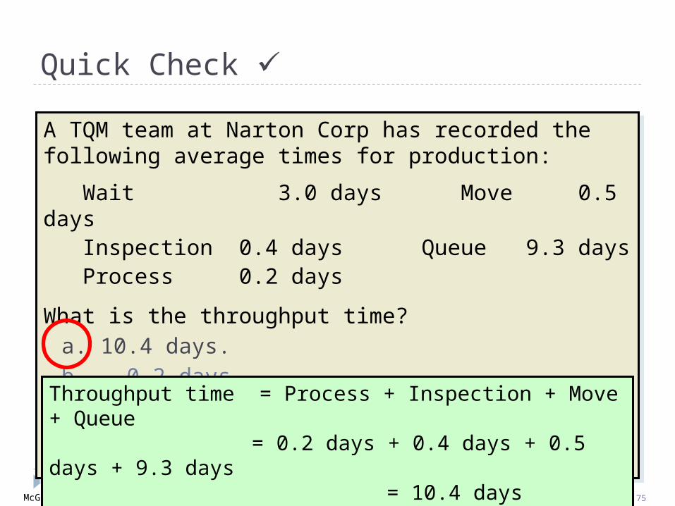
A TQM team at Narton Corp has recorded the following average times for production:
Wait 3.0 days Move 0.5 days Inspection 0.4 days Queue 9.3 days Process 0.2 days
What is the throughput time? a. 10.4 days.b. 0.2 days.c. 4.1 days.d. 13.4 days.
A TQM team at Narton Corp has recorded the following average times for production:
Wait 3.0 days Move 0.5 days Inspection 0.4 days Queue 9.3 days Process 0.2 days
What is the throughput time? a. 10.4 days.b. 0.2 days.c. 4.1 days.d. 13.4 days.
Quick Check
Throughput time = Process + Inspection + Move + Queue = 0.2 days + 0.4 days + 0.5 days + 9.3 days = 10.4 days

McGraw-Hill/Irwin Slide 76
Quick Check
A TQM team at Narton Corp has recorded the following average times for production:
Wait 3.0 days Move 0.5 days Inspection 0.4 days Queue 9.3 days Process 0.2 days
What is the Manufacturing Cycle Efficiency (MCE)? a. 50.0%.b. 1.9%.c. 52.0%.d. 5.1%.
A TQM team at Narton Corp has recorded the following average times for production:
Wait 3.0 days Move 0.5 days Inspection 0.4 days Queue 9.3 days Process 0.2 days
What is the Manufacturing Cycle Efficiency (MCE)? a. 50.0%.b. 1.9%.c. 52.0%.d. 5.1%.

McGraw-Hill/Irwin Slide 77
A TQM team at Narton Corp has recorded the following average times for production:
Wait 3.0 days Move 0.5 days Inspection 0.4 days Queue 9.3 days Process 0.2 days
What is the Manufacturing Cycle Efficiency (MCE)? a. 50.0%.b. 1.9%.c. 52.0%.d. 5.1%.
A TQM team at Narton Corp has recorded the following average times for production:
Wait 3.0 days Move 0.5 days Inspection 0.4 days Queue 9.3 days Process 0.2 days
What is the Manufacturing Cycle Efficiency (MCE)? a. 50.0%.b. 1.9%.c. 52.0%.d. 5.1%.
Quick Check
MCE = Value-added time ÷ Throughput time
= Process time ÷ Throughput time
= 0.2 days ÷ 10.4 days = 1.9%

McGraw-Hill/Irwin Slide 78
Quick Check
A TQM team at Narton Corp has recorded the following average times for production:
Wait 3.0 days Move 0.5 days Inspection 0.4 days Queue 9.3 days Process 0.2 days
What is the delivery cycle time (DCT)? a. 0.5 days.b. 0.7 days.c. 13.4 days.d. 10.4 days.
A TQM team at Narton Corp has recorded the following average times for production:
Wait 3.0 days Move 0.5 days Inspection 0.4 days Queue 9.3 days Process 0.2 days
What is the delivery cycle time (DCT)? a. 0.5 days.b. 0.7 days.c. 13.4 days.d. 10.4 days.

McGraw-Hill/Irwin Slide 79
A TQM team at Narton Corp has recorded the following average times for production:
Wait 3.0 days Move 0.5 days Inspection 0.4 days Queue 9.3 days Process 0.2 days
What is the delivery cycle time (DCT)? a. 0.5 days.b. 0.7 days.c. 13.4 days.d. 10.4 days.
A TQM team at Narton Corp has recorded the following average times for production:
Wait 3.0 days Move 0.5 days Inspection 0.4 days Queue 9.3 days Process 0.2 days
What is the delivery cycle time (DCT)? a. 0.5 days.b. 0.7 days.c. 13.4 days.d. 10.4 days.
Quick Check
DCT = Wait time + Throughput time = 3.0 days + 10.4 days = 13.4 days

© 2010 The McGraw-Hill Companies, Inc.
Predetermined Overhead Rates and Overhead Analysis in a Standard Costing System
Appendix 11A

McGraw-Hill/Irwin Slide 81
Learning Objective 6
(Appendix 11A)(Appendix 11A)
Compute and interpret the fixed overhead budget and volume
variances.

McGraw-Hill/Irwin Slide 82
Budget variance
Fixed Overhead Budget Variance
ActualFixed
Overhead
FixedOverheadApplied
BudgetedFixed
Overhead
Budgetvariance
Budgetedfixed
overhead
Actualfixed
overhead= –

McGraw-Hill/Irwin Slide 83
Volumevariance
Fixed Overhead Volume Variance
ActualFixed
Overhead
FixedOverheadApplied
BudgetedFixed
Overhead
Volumevariance
Fixedoverheadapplied to
work in process
Budgetedfixed
overhead= –

McGraw-Hill/Irwin Slide 84
FPOHR = Fixed portion of the predetermined overhead rate DH = Denominator hours SH = Standard hours allowed for actual output
SH × FRDH × FR
Fixed Overhead Volume Variance
ActualFixed
Overhead
FixedOverheadApplied
BudgetedFixed
Overhead
Volume variance FPOHR × (DH – SH)=
Volumevariance

McGraw-Hill/Irwin Slide 85
Computing Fixed Overhead Variances
Budgeted production 30,000 units Standard machine-hours per unit 3 hours Budgeted machine-hours 90,000 hours Actual production 28,000 units Standard machine-hours allowed for the actual production 84,000 hours Actual machine-hours 88,000 hours
Production and Machine-Hour DataColaCo

McGraw-Hill/Irwin Slide 86
Computing Fixed Overhead Variances
Budgeted variable manufacturing overhead 90,000$ Budgeted fixed manufacturing overhead 270,000 Total budgeted manufacturing overhead 360,000$
Actual variable manufacturing overhead 100,000$ Actual fixed manufacturing overhead 280,000 Total actual manufacturing overhead 380,000$
ColaCoCost Data

McGraw-Hill/Irwin Slide 87
Predetermined Overhead Rates
Predetermined overhead rate
Estimated total manufacturing overhead costEstimated total amount of the allocation base
=
Predetermined overhead rate
$360,00090,000 Machine-hours
=
Predetermined overhead rate
= $4.00 per machine-hour

McGraw-Hill/Irwin Slide 88
Predetermined Overhead Rates
Variable component of thepredetermined overhead rate
$90,00090,000 Machine-hours
=
Variable component of thepredetermined overhead rate
= $1.00 per machine-hour
Fixed component of thepredetermined overhead rate
$270,00090,000 Machine-hours
=
Fixed component of thepredetermined overhead rate
= $3.00 per machine-hour

McGraw-Hill/Irwin Slide 89
Applying Manufacturing Overhead
Overheadapplied
Predetermined overhead rate
Standard hours allowedfor the actual output
= ×
Overheadapplied
$4.00 permachine-hour
84,000 machine-hours= ×
Overheadapplied
$336,000=

McGraw-Hill/Irwin Slide 90
Computing the Budget Variance
Budgetvariance
Budgetedfixed
overhead
Actualfixed
overhead= –
Budgetvariance
= $280,000 – $270,000
Budgetvariance
= $10,000 Unfavorable

McGraw-Hill/Irwin Slide 91
Computing the Volume Variance
Volumevariance
Fixedoverheadapplied to
work in process
Budgetedfixed
overhead= –
Volumevariance
= $18,000 Unfavorable
Volumevariance
= $270,000 –$3.00 per
machine-hour( ×$84,000
machine-hours)

McGraw-Hill/Irwin Slide 92
Computing the Volume Variance
FPOHR = Fixed portion of the predetermined overhead rate DH = Denominator hours SH = Standard hours allowed for actual output
Volume variance FPOHR × (DH – SH)=
Volumevariance
=$3.00 per
machine-hour (×90,000
mach-hours–
84,000mach-hours)
Volumevariance
= 18,000 Unfavorable

McGraw-Hill/Irwin Slide 93
A Pictorial View of the Variances
ActualFixed
Overhead
Fixed OverheadApplied to
Work in Process
BudgetedFixed
Overhead
252,000270,000280,000
Total variance, $28,000 unfavorable
Budget variance,$10,000 unfavorable
Volume variance,$18,000 unfavorable

McGraw-Hill/Irwin Slide 94
Fixed Overhead Variances –A Graphic Approach
Let’s look at a graph showing fixed overhead
variances. We will use ColaCo’s
numbers from the previous example.

McGraw-Hill/Irwin Slide 95
Graphic Analysis of FixedOverhead Variances
Machine-hours (000)
Budget$270,000
90
Denominatorhours
00
Fixed overhead applied at
$3.00 per standard hour
McGraw-Hill/Irwin Slide 96
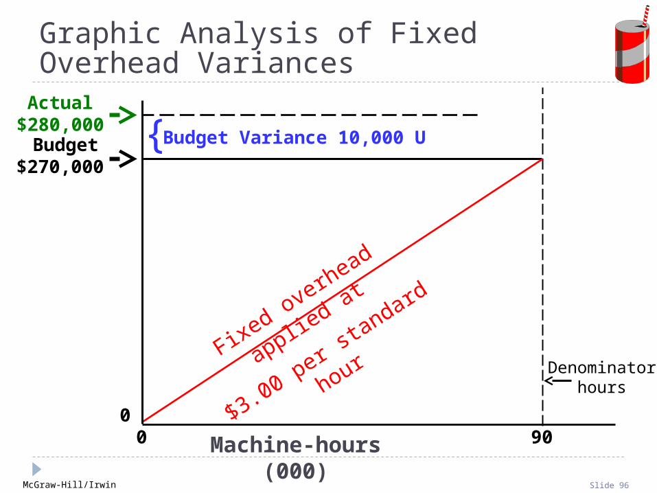
Graphic Analysis of FixedOverhead Variances
Actual$280,000
Machine-hours (000)
Budget$270,000
90
Denominatorhours
00
Fixed overhead applied at
$3.00 per standard hour
Budget Variance 10,000 U{

McGraw-Hill/Irwin Slide 97
Actual$280,000
Applied$252,000
Machine-hours (000)
Budget$270,000
Graphic Analysis of FixedOverhead Variances
908400
Standardhours
Fixed overhead applied at
$3.00 per standard hour
Denominatorhours
Budget Variance 10,000 U
Volume Variance 18,000 U
{{

McGraw-Hill/Irwin Slide 98
Reconciling Overhead Variances and Underapplied or Overapplied Overhead
In a standardcost system:
Unfavorablevariances are equivalent
to underapplied overhead.
Favorablevariances are equivalentto overapplied overhead.
The sum of the overhead variancesequals the under- or overapplied
overhead cost for the period.

McGraw-Hill/Irwin Slide 99
Reconciling Overhead Variances and Underapplied or Overapplied Overhead
Predetermined overhead rate (a) 4.00$ per machine-hour Standard hours allowed for the actual output (b) 84,000 machine hours Manufacturing overhead applied (a) × (b) 336,000$ Actual manufacturing overhead 380,000$ Manufacturing overhead underapplied or overapplied 44,000$ underapplied
Computation of Underapplied OverheadColaCo

McGraw-Hill/Irwin Slide 100
Computing the Variable Overhead Variances
Variable manufacturing overhead rate varianceVMRV = (AH × AR) – (AH × SR) = $100,000 – (88,000 hours × $1.00 per hour) = $12,000 unfavorable

McGraw-Hill/Irwin Slide 101
Computing the Variable Overhead Variances
Variable manufacturing overhead efficiency varianceVMEV = (AH × SR) – (SH × SR) = $88,000 – (84,000 hours × $1.00 per hour) = $4,000 unfavorable

McGraw-Hill/Irwin Slide 102
Computing the Sum of All Variances
Variable overhead rate variance 12,000$ U Variable overhead efficiency variance 4,000 U Fixed overhead budget variance 10,000 U Fixed overhead volume variance 18,000 U Total of the overhead variances 44,000$ U
Computing the Sum of All variancesColaCo

© 2010 The McGraw-Hill Companies, Inc.
Journal Entriesto Record Variances
Appendix 11B

McGraw-Hill/Irwin Slide 104
Learning Objective 7
(Appendix 11B)(Appendix 11B)
Prepare journal entriesPrepare journal entriesto record standardto record standard
costs and variances. costs and variances.

McGraw-Hill/Irwin Slide 105
Appendix 11BJournal Entries to Record Variances
We will use information from the Glacier Peak Outfittersexample presented earlier in the chapter to illustrate journal
entries for standard cost variances. Recall the following:
Material
AQ × AP = $1,029AQ × SP = $1,050SQ × SP = $1,000MPV = $21 FMQV = $50 U
Material
AQ × AP = $1,029AQ × SP = $1,050SQ × SP = $1,000MPV = $21 FMQV = $50 U
Labor
AH × AR = $26,250AH × SR = $25,000SH × SR = $24,000LRV = $1,250 ULEV = $1,000 U
Labor
AH × AR = $26,250AH × SR = $25,000SH × SR = $24,000LRV = $1,250 ULEV = $1,000 U
Now, let’s prepare the entries to recordthe labor and material variances.

McGraw-Hill/Irwin Slide 106
GENERAL JOURNAL Page 4
Date DescriptionPost. Ref. Debit Credit
Raw Materials 1,050
Materials Price Variance 21
Accounts Payable 1,029
To record the purchase of material
Work in Process 1,000
Materials Quantity Variance 50
Raw Materials 1,050
To record the use of material
Appendix 11BRecording Material Variances

McGraw-Hill/Irwin Slide 107
GENERAL JOURNAL Page 4
Date DescriptionPost. Ref. Debit Credit
Work in Process 24,000
Labor Rate Variance 1,250
Labor Efficiency Variance 1,000
Wages Payable 26,250
To record direct labor
Appendix 11BRecording Labor Variances

McGraw-Hill/Irwin Slide 108
Cost Flows in a Standard Cost System
Inventories are recorded at standard cost.
Variances are recorded as follows: Favorable variances are credits, representing
savings in production costs. Unfavorable variances are debits, representing
excess production costs.
Standard cost variances are usually closed out to cost of goods sold. Unfavorable variances increase cost of goods sold. Favorable variances decrease cost of goods sold.

McGraw-Hill/Irwin Slide 109
End of Chapter 11