1

PERFORMANCE EVALUATION OF SURFACE INFILTRATION TRENCHES AND ANISOTROPY DETERMINATION OF WASTE FOR MUNCIPAL SOLID WASTE

LANDFILLS

By

KARAMJIT SINGH

A THESIS PRESENTED TO THE GRADUATE SCHOOL OF THE UNIVERSITY OF FLORIDA IN PARTIAL FULFILLMENT

OF THE REQUIREMENTS FOR THE DEGREE OF MASTER OF SCIENCE

UNIVERSITY OF FLORIDA

2010

2

© 2010 Karamjit Singh

3

To my parents and my loving girlfriend

4

ACKNOWLEDGMENTS

I would like to thank my committee chairman Dr. Timothy G. Townsend for his guidance

and encouragement though the research. I am and will always be indebted to him for training me

for the professional world. I would also like to thank Dr. Michael D. Annable and Dr. Louis H.

Motz for their participation and guidance in completing my research. I am thankful to Darrell

O’Neal, Executive Director, Perry Kent and Lydia Greene of NRSWA for their guidance,

support and special thanks go to Richard Crews and David Mckinney for their support

throughout the construction of my project. I would like to thank Dr. Pradeep Jain, Dr. Ravi

Kadambala, Antonio, Youngmin Cho, Shrawan Singh, Dr. Hwidong Kim, Dr. Jae Hac and Dr.

Qiyong Xu for their assistance and cooperation in this work. I would also like to thank Mark G.

Roberts for his support during the last phase of thesis writing.

Last, but not least, I would like to thank my girlfriend, Loveenia Gulati, for her

understanding and love during the past few years. Her support and encouragement was in the end

what made this thesis possible. My parents, Harmeet Singh and Tejinder Kaur receive my

deepest gratitude and love for their dedication and the many years of support during my

undergraduate studies that provided the foundation for this work.

5

TABLE OF CONTENTS

page

ACKNOWLEDGMENTS.................................................................................................................... 4

LIST OF TABLES................................................................................................................................ 7

LIST OF FIGURES .............................................................................................................................. 7

ABSTRACT .......................................................................................................................................... 8

CHAPTER

1 INTRODUCTION....................................................................................................................... 11

1.1 Background ........................................................................................................................... 11 1.2 Problem Statement ................................................................................................................ 12 1.3 Research Objectives .............................................................................................................. 14 1.4 Research Approach ............................................................................................................... 15 1.5 Organization of Thesis .......................................................................................................... 16

2 ANISOTROPY DETERMINATION OF LANDFILLED MUNCIAL SOLID WASTE ...... 17

2.1 Introduction ........................................................................................................................... 17 2.2 Materials and Methods ......................................................................................................... 19

2.2.1 Experimental Approach ............................................................................................. 19 2.2.2 Field Experiments....................................................................................................... 20 2.2.3 Modeling ..................................................................................................................... 21 2.2.4 Anisotropy Estimation ............................................................................................... 23

2.3 Results and Discussions........................................................................................................ 24 2.3.1 Field Results ............................................................................................................... 24 2.3.2 Simulation Results...................................................................................................... 25 2.3.3 Anisotropy Estimation ............................................................................................... 27 2.3.4 Verification of Results ............................................................................................... 29

2.4 Conclusions ........................................................................................................................... 30

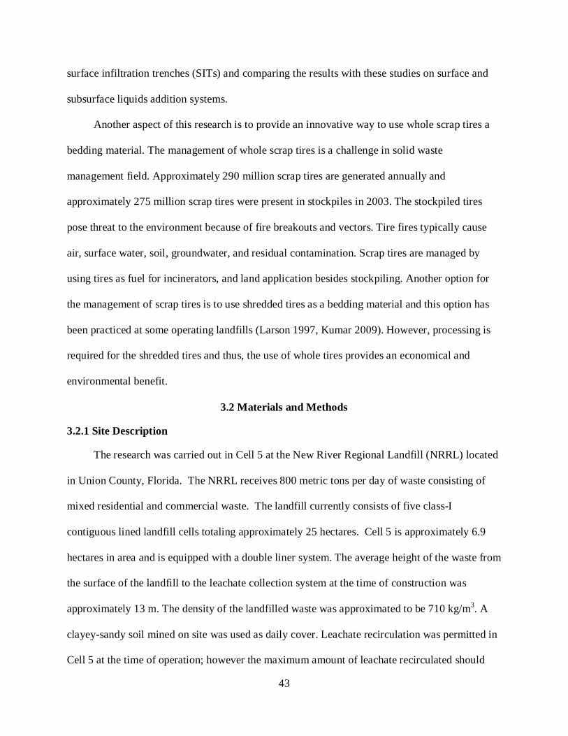
3 PERFORMANCE EVALUATION OF SURFACE INFILTRATION TRENCHES WITH WHOLE TIRES AS A BEDDING MEDIA.................................................................. 42

3.1 Introduction ........................................................................................................................... 42 3.2 Materials and Methods ......................................................................................................... 43

3.2.1 Site Description .......................................................................................................... 43 3.2.2 Installation and Operation of SITs ............................................................................ 44 3.2.3 Modeling ..................................................................................................................... 45 3.2.4 Hydraulic Conductivity Estimation ........................................................................... 47 3.2.5 Model Limitations ...................................................................................................... 47

3.3 Results and Discussion ......................................................................................................... 47

6

3.3.1 Performance of SITs .................................................................................................. 47 3.3.2 Hydraulic Conductivity Estimation ........................................................................... 49 3.3.3 Pros and Cons of SITs ................................................................................................ 50

3.4 Conclusions ........................................................................................................................... 51

4 SUMMARY, CONCLUSIONS, AND RECOMMENDATIONS ........................................... 60

4.1 Summary................................................................................................................................ 60 4.2 Conclusions ........................................................................................................................... 61 4.3 Recommendations ................................................................................................................. 61

APPENDIX

A SUPPLEMENTAL FIGURES FOR CHAPTER 2 ................................................................... 63

B CONSTRUCTION PHOTOGRAPHS FOR CHAPTER 3 ...................................................... 74

LIST OF REFERENCES ................................................................................................................... 84

BIOGRAPHICAL SKETCH ............................................................................................................. 88

7

LIST OF TABLES Table page

2-1 Parameters used for the numerical modeling ....................................................................... 32

2-2 Hydraulic conductivity of different layers with respect to layer 2...................................... 32

2-3 Comparison of field data and simulation data for the first scenario ................................... 33

2-4 Comparison of field data and simulation data for the second scenario .............................. 33

3-1 Parameters used for numerical modeling.............................................................................. 52

3-2 Compilation of field and modeling results ........................................................................... 52

8

LIST OF FIGURES Figure page

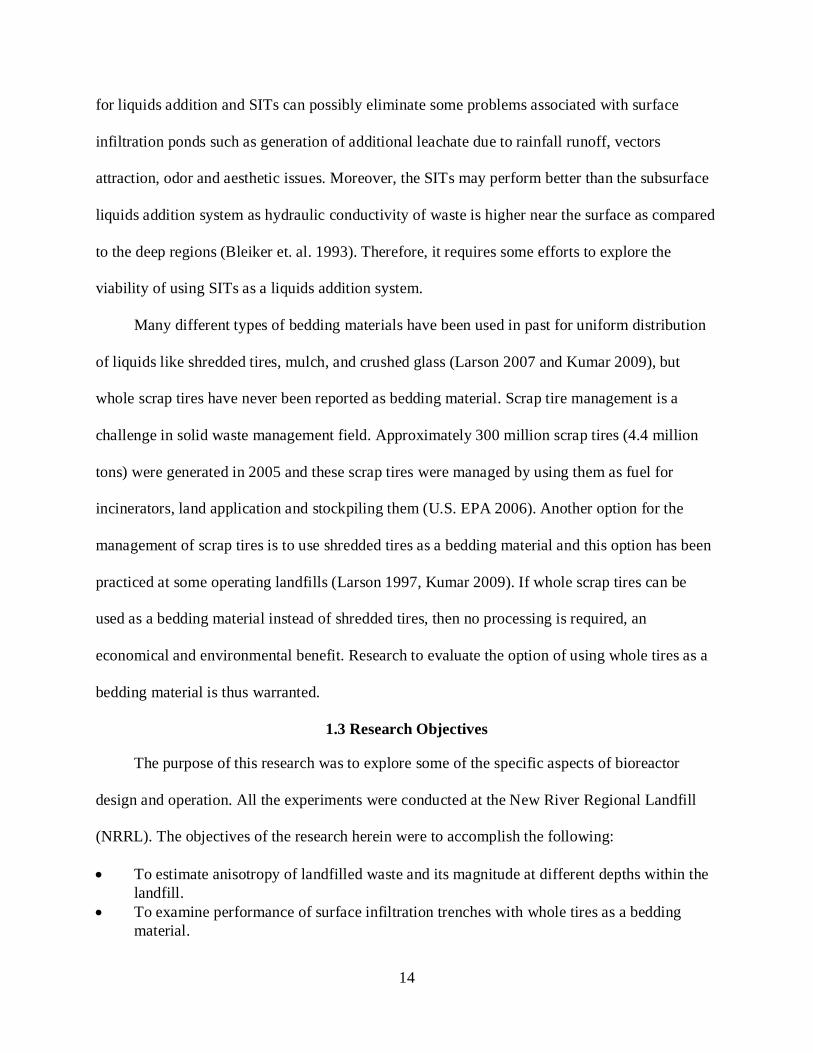
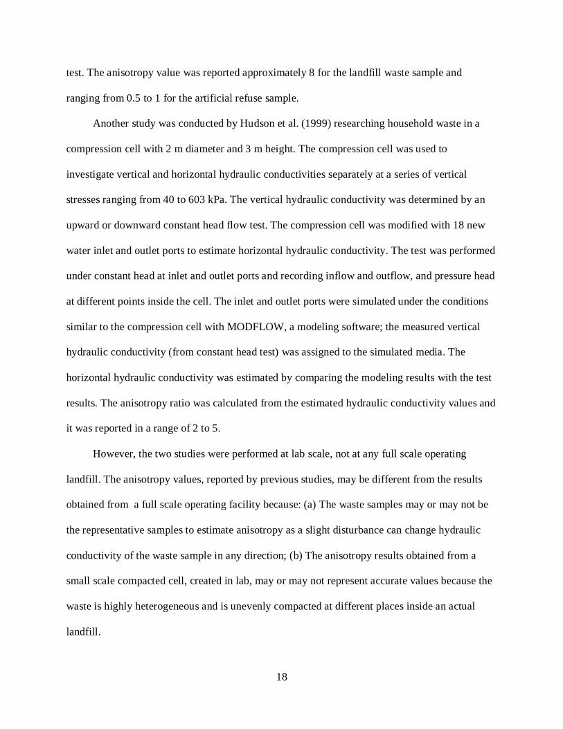
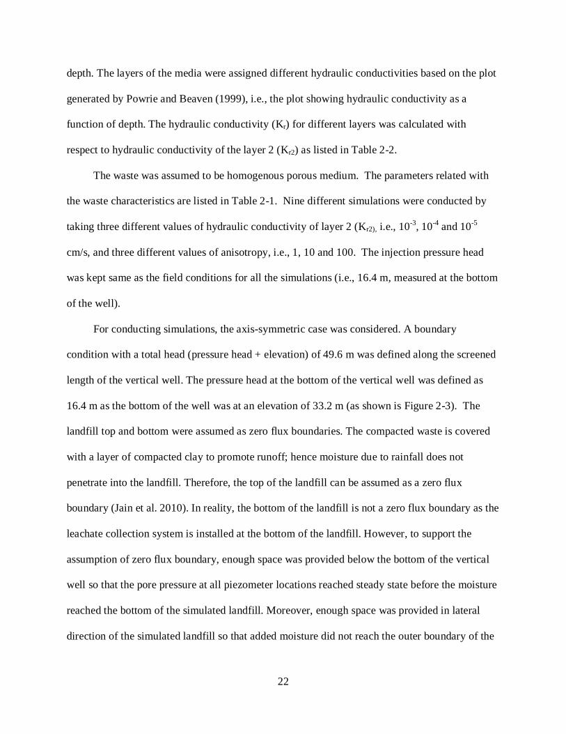
2-1 A) New River Regional Landfill (NRRL) showing the area which contains the moisture addition and the piezometer wells; B) the close up of the liquids addition wells and piezometer wells in the research area................................................................... 34

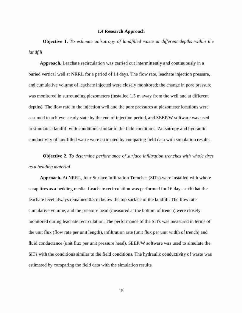
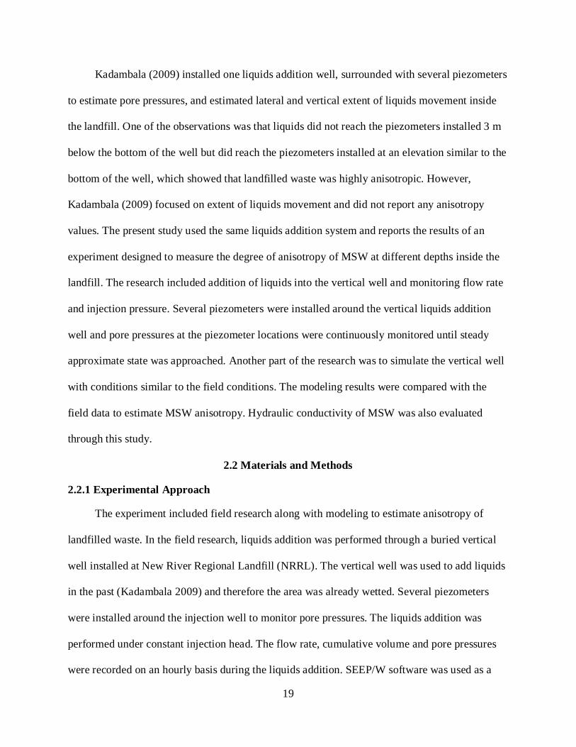
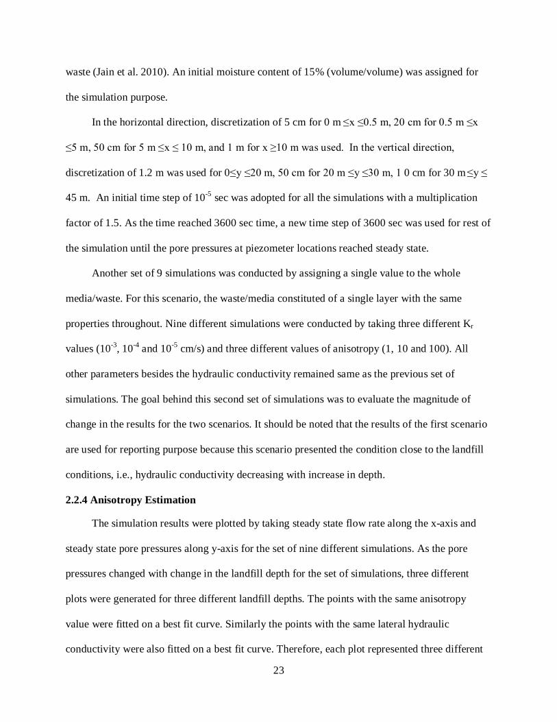
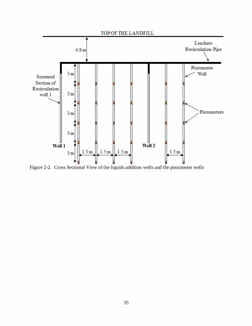
2-2 Cross Sectional View of the liquids addition wells and the piezometer wells ................... 35

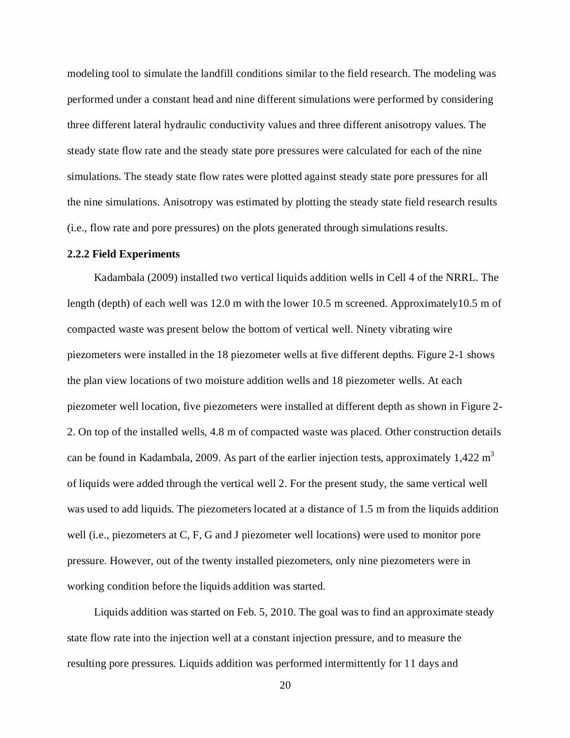
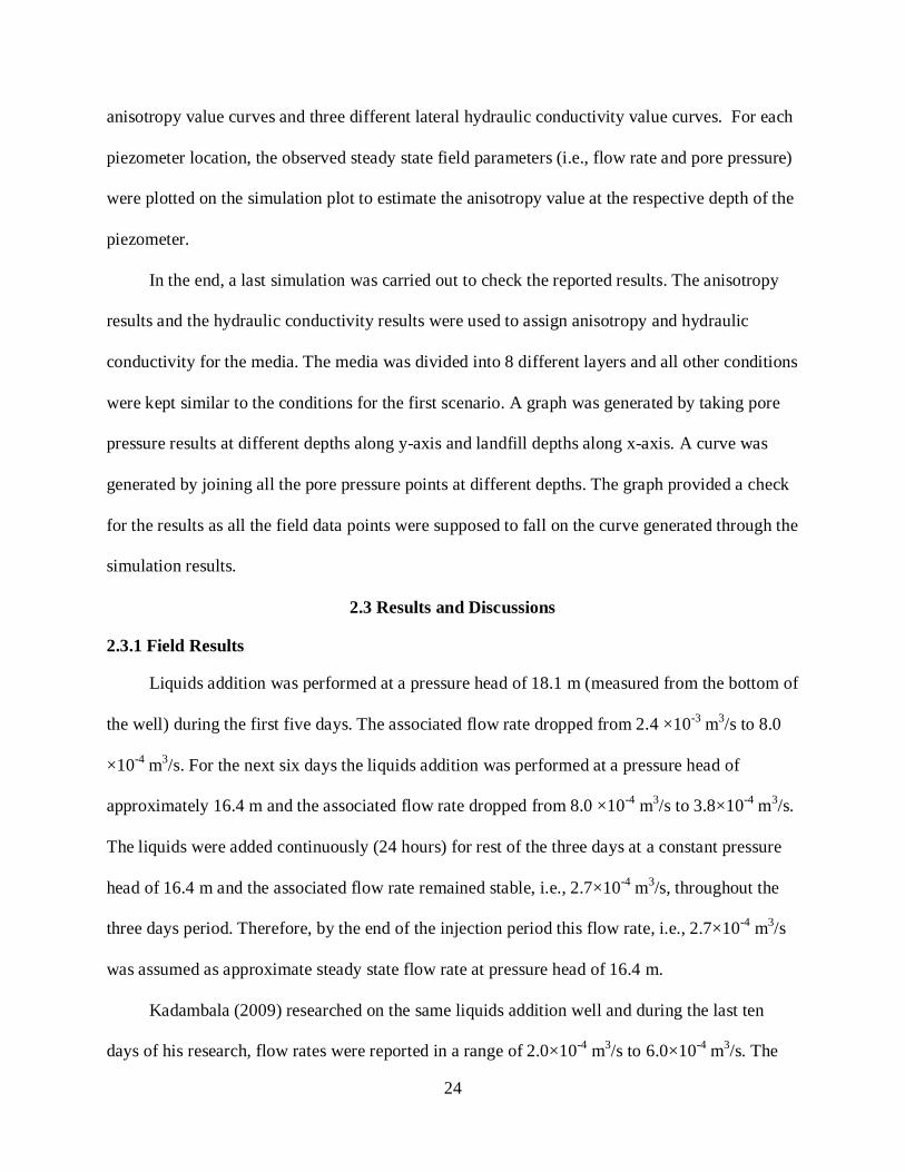
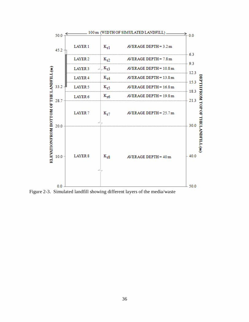
2-3 Simulated landfill showing different layers of the media/waste ......................................... 36

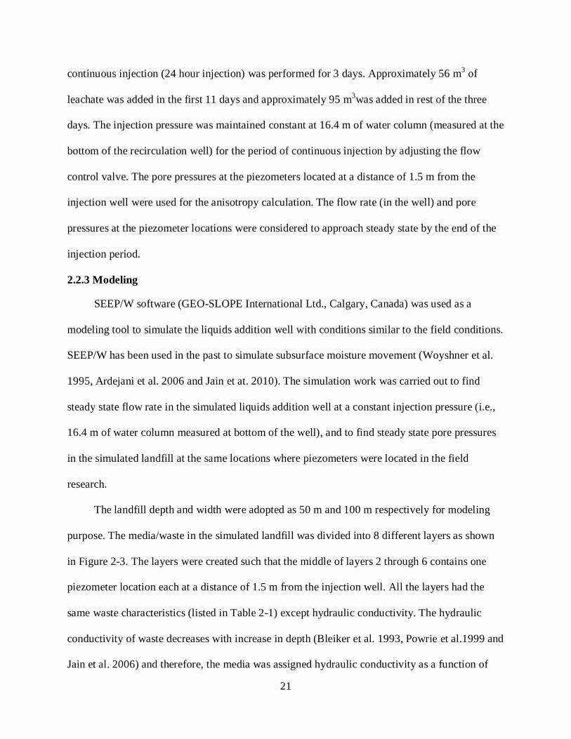
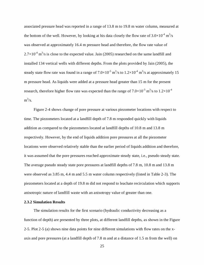
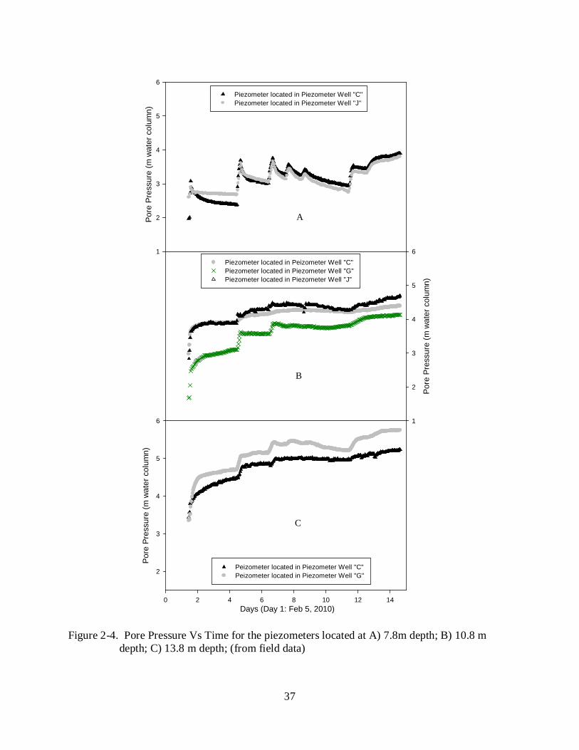
2-4 Pore Pressure Vs Time for the piezometers located at A) 7.8m depth; B) 10.8 m depth; C) 13.8 m depth; (from field data) ............................................................................. 37

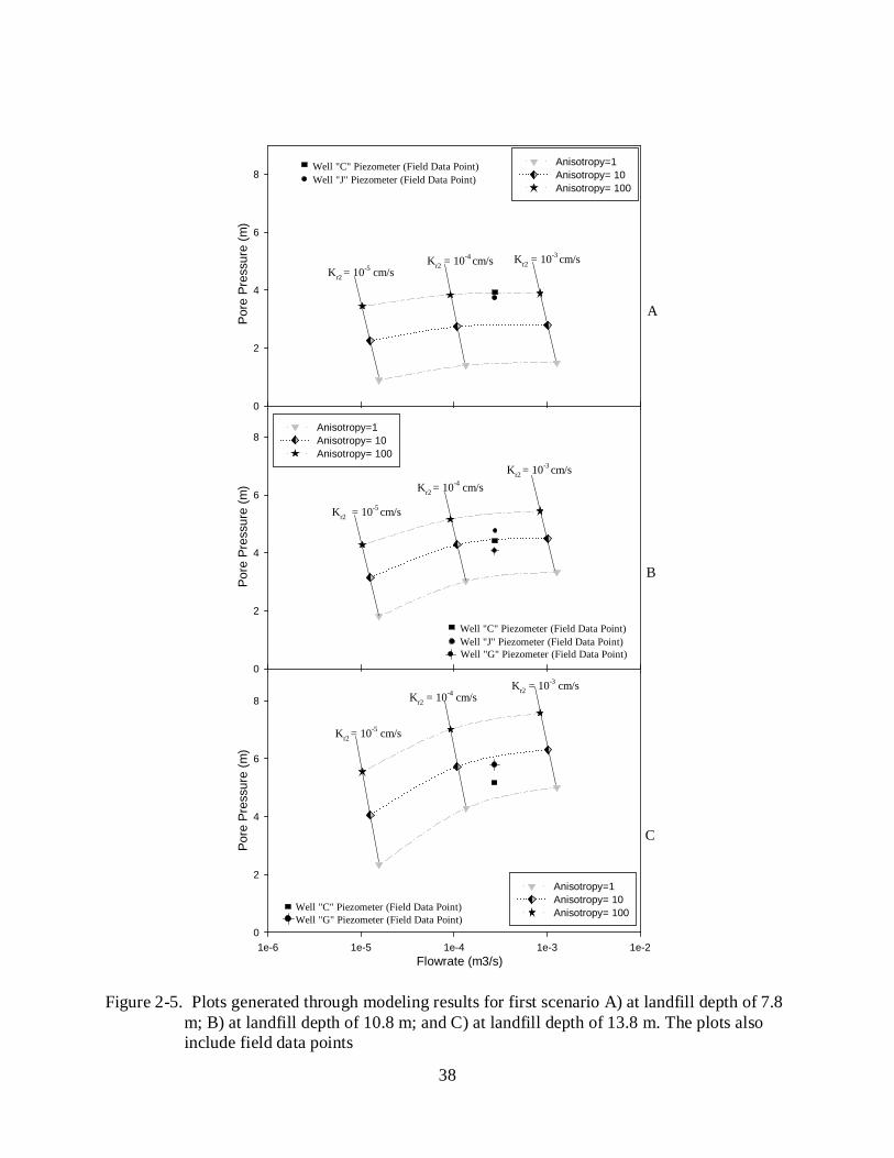
2-5 Plots generated through modeling results for first scenario A) at landfill depth of 7.8 m; B) at landfill depth of 10.8 m; and C) at landfill depth of 13.8 m. The plots also include field data points ......................................................................................................... 38

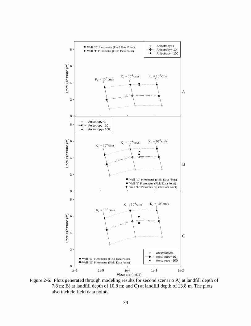
2-6 Plots generated through modeling results for second scenario A) at landfill depth of 7.8 m; B) at landfill depth of 10.8 m; and C) at landfill depth of 13.8 m. The plots also include field data points ................................................................................................. 39

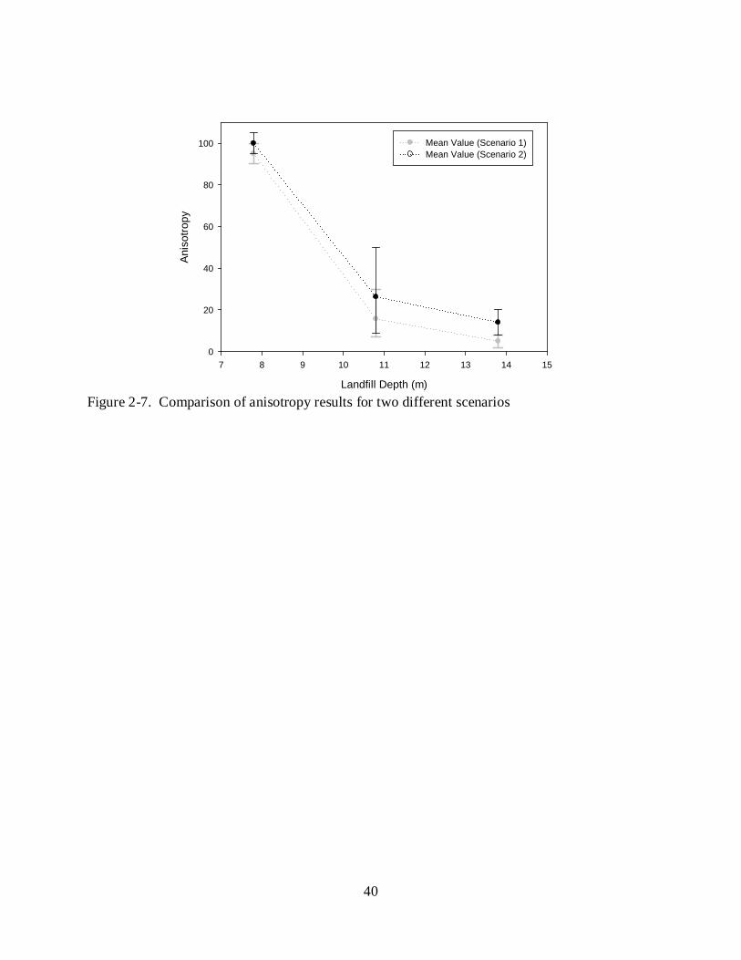
2-7 Comparison of anisotropy results for two different scenarios............................................. 40

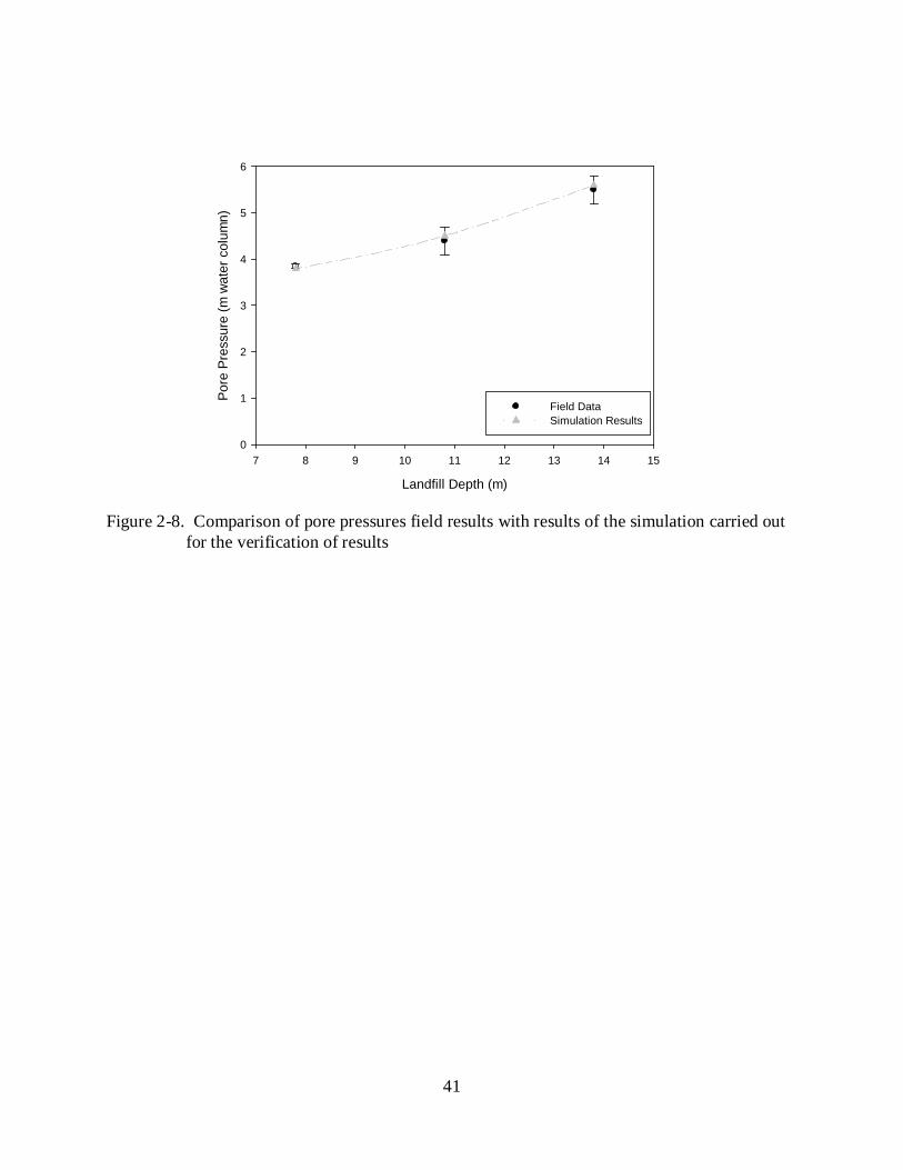
2-8 Comparison of pore pressures field results with results of the simulation carried out for the verification of results ................................................................................................. 41

3-1 Plan View of Cell 5 of New River Regional Landfill showing locations of the Surface Infiltration Trenches ................................................................................................. 53

3-2 Configuration of whole scrap tires used as a bedding media in the surface infiltration trenches: (a) Plan View; (b) Cross Sectional View along width; and (c) Cross Sectional View along length of the trench ............................................................................ 54

3-3 Simulated landfill with showing A) dimensions of the simulated landfill and location of the SIT; B) closer look of the SIT .................................................................................... 55

3-4 Flow rate and pressure head data with respect to time for A) 15 m trench; B) 30 m trench; C) 45 m trench; and D) the second 45 m trench. ..................................................... 56

3-5 Flow rate and pressure head data with respect to cumulative volume for A) 15 m trench; B) 30 m trench; C) 45 m trench; and D) the second 45 m trench. .......................... 57

3-6 Plot generated from the modeling results ............................................................................. 58

3-7 Flux values from field data plotted on the plot generated by modeling results for A)15 m trench; B) 30 m trench; C) 45 m trench; and D) the second 45 m trench. ............ 59

9

Abstract of Thesis Presented to the Graduate School of the University of Florida in Partial Fulfillment of the

Requirements for the Master of Science

PERFORMANCE EVALUATION OF SURFACE INFILTRATION TRENCHES AND ANISOTROPY DETERMINATION OF WASTE FOR MUNCIPAL SOLID WASTE

LANDFILLS

By

Karamjit Singh

December 2010 Chair: Timothy G. Townsend Major: Environmental Engineering Sciences

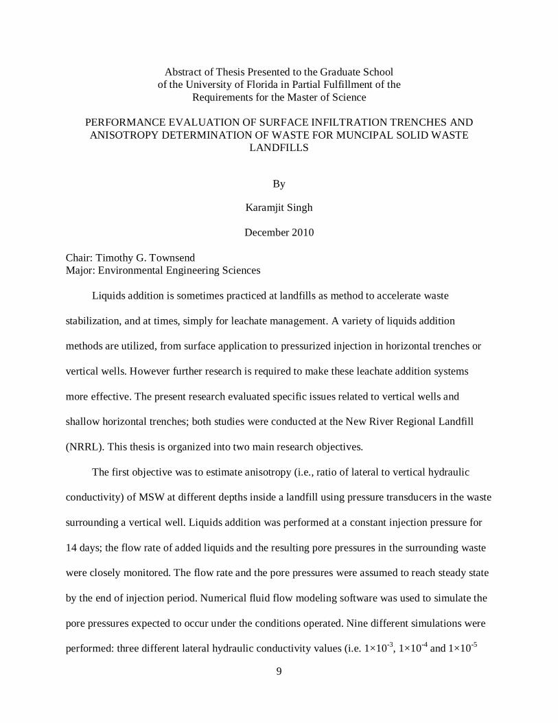
Liquids addition is sometimes practiced at landfills as method to accelerate waste

stabilization, and at times, simply for leachate management. A variety of liquids addition

methods are utilized, from surface application to pressurized injection in horizontal trenches or

vertical wells. However further research is required to make these leachate addition systems

more effective. The present research evaluated specific issues related to vertical wells and

shallow horizontal trenches; both studies were conducted at the New River Regional Landfill

(NRRL). This thesis is organized into two main research objectives.

The first objective was to estimate anisotropy (i.e., ratio of lateral to vertical hydraulic

conductivity) of MSW at different depths inside a landfill using pressure transducers in the waste

surrounding a vertical well. Liquids addition was performed at a constant injection pressure for

14 days; the flow rate of added liquids and the resulting pore pressures in the surrounding waste

were closely monitored. The flow rate and the pore pressures were assumed to reach steady state

by the end of injection period. Numerical fluid flow modeling software was used to simulate the

pore pressures expected to occur under the conditions operated. Nine different simulations were

performed: three different lateral hydraulic conductivity values (i.e. 1×10-3, 1×10-4 and 1×10-5

10

cm/s) and three different anisotropy values (i.e. 1, 10 and 100). The field data (i.e., approximate

steady state flow rate and pore pressures) were compared with the simulation results to estimate

the hydraulic conductivity and the anisotropy. The anisotropy values were found ranging from 2

to 100 with an average value of 36.

The second objective was to evaluate the performance of surface infiltration trenches

(SITs). Four SITs, with different lengths, were installed at NRRL with whole tires as a bedding

media. To construct the SITs, whole scrap tires were tied together face to face with nylon rope

and then installed in 1.2 m deep excavated trenches by placing a 7.6 cm perforated HDPE pipe in

the middle of tied tires. The perforated pipe was connected to the header pipe and liquids

addition was performed for 16 days after covering the trench with 0.3 m of compacted clay. The

performance of the SITs was measured in terms of the unit flux (flow rate per unit length),

infiltration rate (unit flux per unit width of trench) and fluid conductance (unit flux per unit

pressure head). The unit flux was found in a range of 8.0×10-6 m2/s to 1.1×10-5 m2/s, the

infiltration rate ranged from 8.0×10-6 m/s to 1.1×10-5 m/s, and fluid conductance ranged from

8.9×10-6 m/s to 1.2×10-5 m/s. The hydraulic conductivity of the waste surrounding the trenches

was also estimated by comparing the field results with modeling results. The modeling was

performed under the conditions similar to the field conditions and the average vertical hydraulic

conductivity was found as 2.0×10-5 cm/s at an anisotropy ratio of 100.

11

CHAPTER 1 INTRODUCTION

1.1 Background

Municipal solid waste (MSW) generation in the United States increased from 88.1 million

tons in the year 1960 to 254.1 million tons in 2007 (an 188% increase in 47 years; U.S. EPA

2007). Approximately 93% of MSW was disposed of in landfills in 1960, and while this has

decreased over time (54% of MSW was landfilled in 2007), well over 100 million tons of MSW

remains landfilled in the U.S. every year (U.S. EPA 2008). In the last two decades, engineered

landfills have evolved from being open dumps with negligible control, to controlled and

sophisticated containment systems (Kadambala 2009). Typically, the landfills in the United

States are designed and operated in accordance with the requirements of Subtitle D of the

Resource Conservation and Recovery Act (RCRA). These landfills are equipped with a liner and

a leachate collection and removal system. The waste in these landfills may take a long time to

degrade or decompose and hence such landfills may require indefinite maintenance. The concept

of bioreactor landfills was introduced to increase the rate of waste degradation in such

landfills (Reinhart and Townsend 1997). A bioreactor landfill operates to rapidly transform and

degrade organic waste.

The increase in waste degradation and stabilization is accomplished through the addition of

liquid (and in some cases, air) to enhance microbial processes (U.S. EPA 2007). Bioreactor

landfill configurations include anaerobic bioreactors (moisture is added to the waste mass in the

form of recirculated leachate and other sources, in the absence of oxygen, to obtain optimal

moisture levels), aerobic bioreactors (adding liquids along with air into the landfill in a

controlled manner) and hybrid bioreactors (accelerates waste degradation by employing a

sequential aerobic-anaerobic treatment to rapidly degrade organics).

12

Potential bioreactor landfill advantages include faster decomposition and biological

stabilization of waste, a decrease in toxicity and mobility of waste, a reduction in leachate

disposal costs, a gain in landfill space due to decomposition of waste, an increase in landfill gas

production (energy source), and reduced post-closure care effort and costs (Jain 2005).

Bioreactor landfills also have several possible problems, including a reduction in MSW shear

strength (and possible slope stability concerns), leachate breakouts from the sides of the landfill,

an increase in the leachate head build up on the liner, and an increase in uncontrolled landfill gas

emissions (Khire et al. 2006, Reinhart and Townsend 1997). Over the past several decades,

investigators have researched various aspects of bioreactor processes to make these systems a

more viable option for solid waste management (Pohland 1975, 1980, Pohland et al. 1986,

Townsend et al. 1996, Reinhart et al. 1997, 2002, Mehta et al. 2002). Even though a significant

amount of research has been performed on bioreactor landfills, additional research is required to

make this technology more efficient.

1.2 Problem Statement

Several full-scale operations have been implemented in U.S. to evaluate the performance

of bioreactor landfills (Pacey et al. 1999, Jain et al. 2005 and Benson et al. 2007). One such full-

scale bioreactor is at the New River Regional Landfill (NRRL) located in Union County, Florida.

The landfill currently consists of five contiguous lined landfill cells totaling approximately 25

hectares. A detailed description of the site and the bioreactor can be found elsewhere (Jain 2005,

Kadambala 2009). Jain et al (2005) evaluated the performance of vertical wells for landfill

leachate recirculation and several lessons were learned that prompted this research. In 2007, nine

vertical well clusters (each having nine vertical wells) were constructed in cell 4 and part of cell

2 and Kadambala (2009) evaluated the performance of modified vertical wells for landfill

leachate recirculation. In 2007, another two 12.2 m deep modified vertical wells were

13

constructed and surrounded by 18 multi-level piezometers; Kadambala (2009) evaluated the

lateral and spatial moisture moment by injecting liquids through one of the two constructed

vertical wells.

There have been a number of laboratory and field studies conducted to measure hydraulic

conductivity of MSW (Shank 1993, Townsend 1995, Gabr 1995, Jain 2005, Koerner and Eith

2005 and Durmusoglu 2006); however, not much information is available on anisotropy of

landfilled waste, defined as the ratio of lateral (horizontal) to vertical hydraulic conductivity.

Landva et al. (1998) reported anisotropy value as 8 and Hudson et al. (1999) reported anisotropy

value in a range of 2 to 5. However, both the studies were conducted on lab scale and may not

represent the actual anisotropy values for a full scale operating landfill. Anisotropy is an

important design parameter because radial (horizontal) and vertical impact zones, created due to

liquids addition, are closely associated with it. When designing a subsurface moisture addition

system, the spacing between vertical wells or horizontal injection lines (HILs) is based upon

impact zones created by moisture addition and thus, anisotropy is one of the most important

parameter to determine spacing. Additional efforts are needed to better determine anisotropy of

landfilled waste.

Both surface and subsurface liquids addition systems are practiced at bioreactor landfills.

Horizontal injection lines and vertical wells are two examples of subsurface liquids additions

systems and considerable research has been conducted on various aspects of these systems

(McCreanor et al. 1996 and 2000, Townsend et al. 1998, McCreanor 1998, Haydar et al. 2004

and 2005, Jain 2005, Larson 2007, Kadambala 2009). Surface infiltration ponds and surface

infiltration trenches are two types of surface liquids addition systems, less research has been

conducted (Townsend et al., 1995). Surface infiltration trenches (SITs) are an inexpensive option

14

for liquids addition and SITs can possibly eliminate some problems associated with surface

infiltration ponds such as generation of additional leachate due to rainfall runoff, vectors

attraction, odor and aesthetic issues. Moreover, the SITs may perform better than the subsurface

liquids addition system as hydraulic conductivity of waste is higher near the surface as compared

to the deep regions (Bleiker et. al. 1993). Therefore, it requires some efforts to explore the

viability of using SITs as a liquids addition system.

Many different types of bedding materials have been used in past for uniform distribution

of liquids like shredded tires, mulch, and crushed glass (Larson 2007 and Kumar 2009), but

whole scrap tires have never been reported as bedding material. Scrap tire management is a

challenge in solid waste management field. Approximately 300 million scrap tires (4.4 million

tons) were generated in 2005 and these scrap tires were managed by using them as fuel for

incinerators, land application and stockpiling them (U.S. EPA 2006). Another option for the

management of scrap tires is to use shredded tires as a bedding material and this option has been

practiced at some operating landfills (Larson 1997, Kumar 2009). If whole scrap tires can be

used as a bedding material instead of shredded tires, then no processing is required, an

economical and environmental benefit. Research to evaluate the option of using whole tires as a

bedding material is thus warranted.

1.3 Research Objectives

The purpose of this research was to explore some of the specific aspects of bioreactor

design and operation. All the experiments were conducted at the New River Regional Landfill

(NRRL). The objectives of the research herein were to accomplish the following:

• To estimate anisotropy of landfilled waste and its magnitude at different depths within the landfill.

• To examine performance of surface infiltration trenches with whole tires as a bedding material.

15

1.4 Research Approach

Objective 1. To estimate anisotropy of landfilled waste at different depths within the

landfill

Approach. Leachate recirculation was carried out intermittently and continuously in a

buried vertical well at NRRL for a period of 14 days. The flow rate, leachate injection pressure,

and cumulative volume of leachate injected were closely monitored; the change in pore pressure

was monitored in surrounding piezometers (installed 1.5 m away from the well and at different

depths). The flow rate in the injection well and the pore pressures at piezometer locations were

assumed to achieve steady state by the end of injection period, and SEEP/W software was used

to simulate a landfill with conditions similar to the field conditions. Anisotropy and hydraulic

conductivity of landfilled waste were estimated by comparing field data with simulation results.

Objective 2. To determine performance of surface infiltration trenches with whole tires

as a bedding material

Approach. At NRRL, four Surface Infiltration Trenches (SITs) were installed with whole

scrap tires as a bedding media. Leachate recirculation was performed for 16 days such that the

leachate level always remained 0.3 m below the top surface of the landfill. The flow rate,

cumulative volume, and the pressure head (measured at the bottom of trench) were closely

monitored during leachate recirculation. The performance of the SITs was measured in terms of

the unit flux (flow rate per unit length), infiltration rate (unit flux per unit width of trench) and

fluid conductance (unit flux per unit pressure head). SEEP/W software was used to simulate the

SITs with the conditions similar to the field conditions. The hydraulic conductivity of waste was

estimated by comparing the field data with the simulation results.

16

1.5 Organization of Thesis

Chapter 2 presents the flow rate and pore pressure results for the field research conducted

on a liquids addition well. The chapter also reports the modeling results performed under the

conditions similar to the field conditions. In the end of the chapter, field and modeling results are

compared to estimate anisotropy of landfilled waste. Chapter 3 discusses flux, infiltration rate

and fluid conductance of the four SITs. The flux, infiltration rate and fluid conductance are

calculated by the flow-pressure field data based on liquids addition experiments on the surface

infiltration trenches. The chapter also reports the hydraulic conductivity of landfilled waste. The

thesis ends with Chapter 4, a summary and a set of conclusions from Chapters 2 and 3, and

includes recommendations for future research. Appendix A presents supplemental figures of

Chapter 2 and Appendix B presents the photographs for the installation of surface infiltration

trenches.

17

CHAPTER 2 ANISOTROPY DETERMINATION OF LANDFILLED MUNCIAL SOLID WASTE

2.1 Introduction

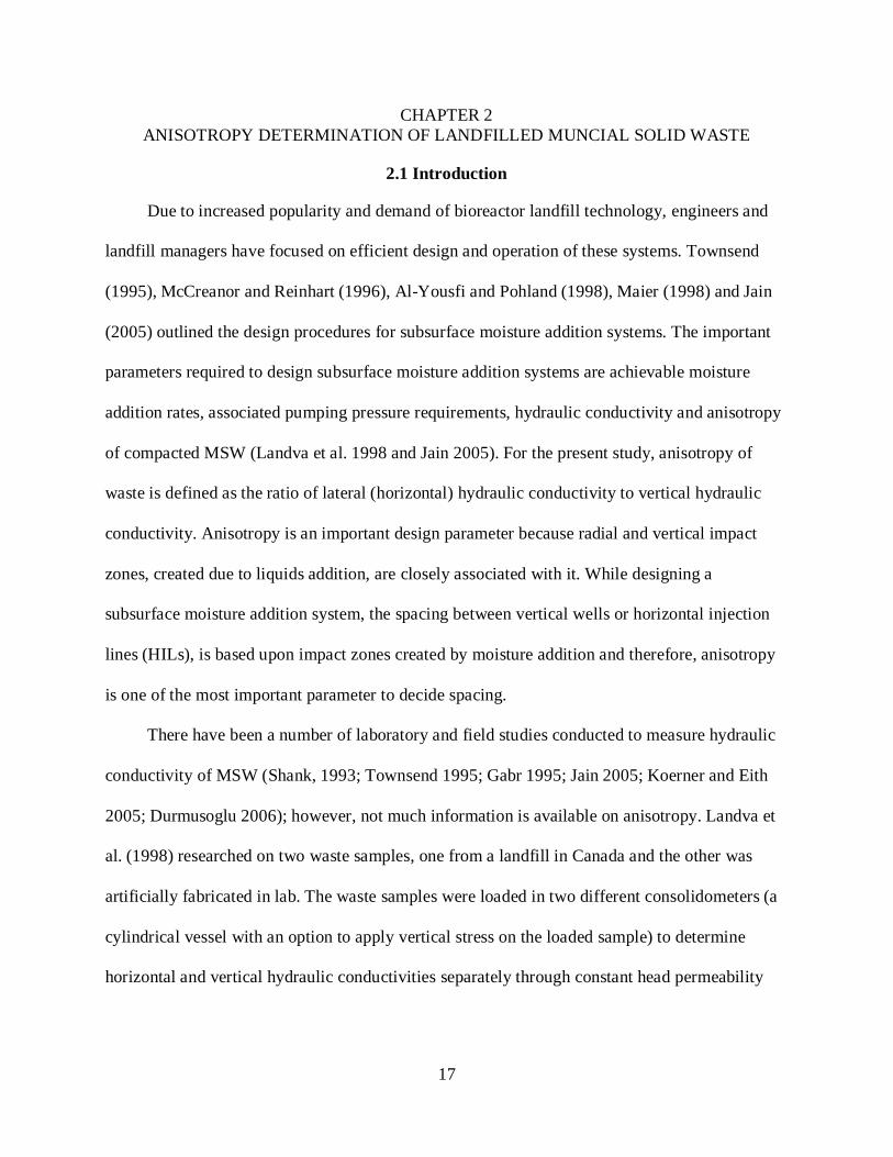
Due to increased popularity and demand of bioreactor landfill technology, engineers and

landfill managers have focused on efficient design and operation of these systems. Townsend

(1995), McCreanor and Reinhart (1996), Al-Yousfi and Pohland (1998), Maier (1998) and Jain

(2005) outlined the design procedures for subsurface moisture addition systems. The important

parameters required to design subsurface moisture addition systems are achievable moisture

addition rates, associated pumping pressure requirements, hydraulic conductivity and anisotropy

of compacted MSW (Landva et al. 1998 and Jain 2005). For the present study, anisotropy of

waste is defined as the ratio of lateral (horizontal) hydraulic conductivity to vertical hydraulic

conductivity. Anisotropy is an important design parameter because radial and vertical impact

zones, created due to liquids addition, are closely associated with it. While designing a

subsurface moisture addition system, the spacing between vertical wells or horizontal injection

lines (HILs), is based upon impact zones created by moisture addition and therefore, anisotropy

is one of the most important parameter to decide spacing.

There have been a number of laboratory and field studies conducted to measure hydraulic

conductivity of MSW (Shank, 1993; Townsend 1995; Gabr 1995; Jain 2005; Koerner and Eith

2005; Durmusoglu 2006); however, not much information is available on anisotropy. Landva et

al. (1998) researched on two waste samples, one from a landfill in Canada and the other was

artificially fabricated in lab. The waste samples were loaded in two different consolidometers (a

cylindrical vessel with an option to apply vertical stress on the loaded sample) to determine

horizontal and vertical hydraulic conductivities separately through constant head permeability

18

test. The anisotropy value was reported approximately 8 for the landfill waste sample and

ranging from 0.5 to 1 for the artificial refuse sample.

Another study was conducted by Hudson et al. (1999) researching household waste in a

compression cell with 2 m diameter and 3 m height. The compression cell was used to

investigate vertical and horizontal hydraulic conductivities separately at a series of vertical

stresses ranging from 40 to 603 kPa. The vertical hydraulic conductivity was determined by an

upward or downward constant head flow test. The compression cell was modified with 18 new

water inlet and outlet ports to estimate horizontal hydraulic conductivity. The test was performed

under constant head at inlet and outlet ports and recording inflow and outflow, and pressure head

at different points inside the cell. The inlet and outlet ports were simulated under the conditions

similar to the compression cell with MODFLOW, a modeling software; the measured vertical

hydraulic conductivity (from constant head test) was assigned to the simulated media. The

horizontal hydraulic conductivity was estimated by comparing the modeling results with the test

results. The anisotropy ratio was calculated from the estimated hydraulic conductivity values and

it was reported in a range of 2 to 5.

However, the two studies were performed at lab scale, not at any full scale operating

landfill. The anisotropy values, reported by previous studies, may be different from the results

obtained from a full scale operating facility because: (a) The waste samples may or may not be

the representative samples to estimate anisotropy as a slight disturbance can change hydraulic

conductivity of the waste sample in any direction; (b) The anisotropy results obtained from a

small scale compacted cell, created in lab, may or may not represent accurate values because the

waste is highly heterogeneous and is unevenly compacted at different places inside an actual

landfill.

19

Kadambala (2009) installed one liquids addition well, surrounded with several piezometers

to estimate pore pressures, and estimated lateral and vertical extent of liquids movement inside

the landfill. One of the observations was that liquids did not reach the piezometers installed 3 m

below the bottom of the well but did reach the piezometers installed at an elevation similar to the

bottom of the well, which showed that landfilled waste was highly anisotropic. However,

Kadambala (2009) focused on extent of liquids movement and did not report any anisotropy

values. The present study used the same liquids addition system and reports the results of an

experiment designed to measure the degree of anisotropy of MSW at different depths inside the

landfill. The research included addition of liquids into the vertical well and monitoring flow rate

and injection pressure. Several piezometers were installed around the vertical liquids addition

well and pore pressures at the piezometer locations were continuously monitored until steady

approximate state was approached. Another part of the research was to simulate the vertical well

with conditions similar to the field conditions. The modeling results were compared with the

field data to estimate MSW anisotropy. Hydraulic conductivity of MSW was also evaluated

through this study.

2.2 Materials and Methods

2.2.1 Experimental Approach

The experiment included field research along with modeling to estimate anisotropy of

landfilled waste. In the field research, liquids addition was performed through a buried vertical

well installed at New River Regional Landfill (NRRL). The vertical well was used to add liquids

in the past (Kadambala 2009) and therefore the area was already wetted. Several piezometers

were installed around the injection well to monitor pore pressures. The liquids addition was

performed under constant injection head. The flow rate, cumulative volume and pore pressures

were recorded on an hourly basis during the liquids addition. SEEP/W software was used as a

20

modeling tool to simulate the landfill conditions similar to the field research. The modeling was

performed under a constant head and nine different simulations were performed by considering

three different lateral hydraulic conductivity values and three different anisotropy values. The

steady state flow rate and the steady state pore pressures were calculated for each of the nine

simulations. The steady state flow rates were plotted against steady state pore pressures for all

the nine simulations. Anisotropy was estimated by plotting the steady state field research results

(i.e., flow rate and pore pressures) on the plots generated through simulations results.

2.2.2 Field Experiments

Kadambala (2009) installed two vertical liquids addition wells in Cell 4 of the NRRL. The

length (depth) of each well was 12.0 m with the lower 10.5 m screened. Approximately10.5 m of

compacted waste was present below the bottom of vertical well. Ninety vibrating wire

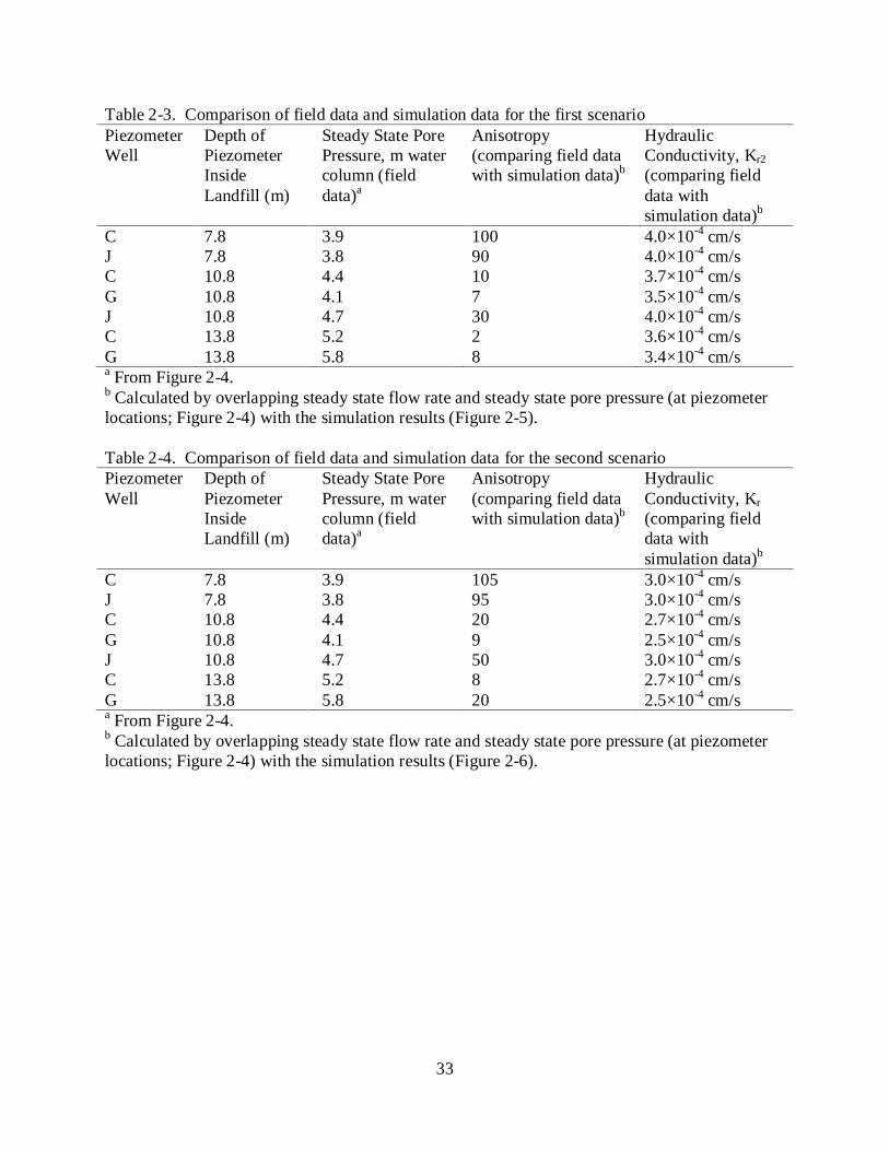
piezometers were installed in the 18 piezometer wells at five different depths. Figure 2-1 shows

the plan view locations of two moisture addition wells and 18 piezometer wells. At each

piezometer well location, five piezometers were installed at different depth as shown in Figure 2-

2. On top of the installed wells, 4.8 m of compacted waste was placed. Other construction details

can be found in Kadambala, 2009. As part of the earlier injection tests, approximately 1,422 m3

of liquids were added through the vertical well 2. For the present study, the same vertical well

was used to add liquids. The piezometers located at a distance of 1.5 m from the liquids addition

well (i.e., piezometers at C, F, G and J piezometer well locations) were used to monitor pore

pressure. However, out of the twenty installed piezometers, only nine piezometers were in

working condition before the liquids addition was started.

Liquids addition was started on Feb. 5, 2010. The goal was to find an approximate steady

state flow rate into the injection well at a constant injection pressure, and to measure the

resulting pore pressures. Liquids addition was performed intermittently for 11 days and

21

continuous injection (24 hour injection) was performed for 3 days. Approximately 56 m3 of

leachate was added in the first 11 days and approximately 95 m3was added in rest of the three

days. The injection pressure was maintained constant at 16.4 m of water column (measured at the

bottom of the recirculation well) for the period of continuous injection by adjusting the flow

control valve. The pore pressures at the piezometers located at a distance of 1.5 m from the

injection well were used for the anisotropy calculation. The flow rate (in the well) and pore

pressures at the piezometer locations were considered to approach steady state by the end of the

injection period.

2.2.3 Modeling

SEEP/W software (GEO-SLOPE International Ltd., Calgary, Canada) was used as a

modeling tool to simulate the liquids addition well with conditions similar to the field conditions.

SEEP/W has been used in the past to simulate subsurface moisture movement (Woyshner et al.

1995, Ardejani et al. 2006 and Jain et at. 2010). The simulation work was carried out to find

steady state flow rate in the simulated liquids addition well at a constant injection pressure (i.e.,

16.4 m of water column measured at bottom of the well), and to find steady state pore pressures

in the simulated landfill at the same locations where piezometers were located in the field

research.

The landfill depth and width were adopted as 50 m and 100 m respectively for modeling

purpose. The media/waste in the simulated landfill was divided into 8 different layers as shown

in Figure 2-3. The layers were created such that the middle of layers 2 through 6 contains one

piezometer location each at a distance of 1.5 m from the injection well. All the layers had the

same waste characteristics (listed in Table 2-1) except hydraulic conductivity. The hydraulic

conductivity of waste decreases with increase in depth (Bleiker et al. 1993, Powrie et al.1999 and

Jain et al. 2006) and therefore, the media was assigned hydraulic conductivity as a function of

22

depth. The layers of the media were assigned different hydraulic conductivities based on the plot

generated by Powrie and Beaven (1999), i.e., the plot showing hydraulic conductivity as a

function of depth. The hydraulic conductivity (Kr) for different layers was calculated with

respect to hydraulic conductivity of the layer 2 (Kr2) as listed in Table 2-2.

The waste was assumed to be homogenous porous medium. The parameters related with

the waste characteristics are listed in Table 2-1. Nine different simulations were conducted by

taking three different values of hydraulic conductivity of layer 2 (Kr2), i.e., 10-3, 10-4 and 10-5

cm/s, and three different values of anisotropy, i.e., 1, 10 and 100. The injection pressure head

was kept same as the field conditions for all the simulations (i.e., 16.4 m, measured at the bottom

of the well).

For conducting simulations, the axis-symmetric case was considered. A boundary

condition with a total head (pressure head + elevation) of 49.6 m was defined along the screened

length of the vertical well. The pressure head at the bottom of the vertical well was defined as

16.4 m as the bottom of the well was at an elevation of 33.2 m (as shown is Figure 2-3). The

landfill top and bottom were assumed as zero flux boundaries. The compacted waste is covered

with a layer of compacted clay to promote runoff; hence moisture due to rainfall does not

penetrate into the landfill. Therefore, the top of the landfill can be assumed as a zero flux

boundary (Jain et al. 2010). In reality, the bottom of the landfill is not a zero flux boundary as the

leachate collection system is installed at the bottom of the landfill. However, to support the

assumption of zero flux boundary, enough space was provided below the bottom of the vertical

well so that the pore pressure at all piezometer locations reached steady state before the moisture

reached the bottom of the simulated landfill. Moreover, enough space was provided in lateral

direction of the simulated landfill so that added moisture did not reach the outer boundary of the

23

waste (Jain et al. 2010). An initial moisture content of 15% (volume/volume) was assigned for

the simulation purpose.

In the horizontal direction, discretization of 5 cm for 0 m ≤x ≤0.5 m, 20 cm for 0.5 m ≤x

≤5 m, 50 cm for 5 m ≤x ≤ 10 m, and 1 m for x ≥10 m was used. In the vertical direction,

discretization of 1.2 m was used for 0 ≤y ≤20 m, 50 cm for 20 m ≤y ≤30 m, 1 0 cm for 30 m ≤y ≤

45 m. An initial time step of 10-5 sec was adopted for all the simulations with a multiplication

factor of 1.5. As the time reached 3600 sec time, a new time step of 3600 sec was used for rest of

the simulation until the pore pressures at piezometer locations reached steady state.

Another set of 9 simulations was conducted by assigning a single value to the whole

media/waste. For this scenario, the waste/media constituted of a single layer with the same

properties throughout. Nine different simulations were conducted by taking three different Kr

values (10-3, 10-4 and 10-5 cm/s) and three different values of anisotropy (1, 10 and 100). All

other parameters besides the hydraulic conductivity remained same as the previous set of

simulations. The goal behind this second set of simulations was to evaluate the magnitude of

change in the results for the two scenarios. It should be noted that the results of the first scenario

are used for reporting purpose because this scenario presented the condition close to the landfill

conditions, i.e., hydraulic conductivity decreasing with increase in depth.

2.2.4 Anisotropy Estimation

The simulation results were plotted by taking steady state flow rate along the x-axis and

steady state pore pressures along y-axis for the set of nine different simulations. As the pore

pressures changed with change in the landfill depth for the set of simulations, three different

plots were generated for three different landfill depths. The points with the same anisotropy

value were fitted on a best fit curve. Similarly the points with the same lateral hydraulic

conductivity were also fitted on a best fit curve. Therefore, each plot represented three different

24

anisotropy value curves and three different lateral hydraulic conductivity value curves. For each

piezometer location, the observed steady state field parameters (i.e., flow rate and pore pressure)

were plotted on the simulation plot to estimate the anisotropy value at the respective depth of the

piezometer.

In the end, a last simulation was carried out to check the reported results. The anisotropy

results and the hydraulic conductivity results were used to assign anisotropy and hydraulic

conductivity for the media. The media was divided into 8 different layers and all other conditions

were kept similar to the conditions for the first scenario. A graph was generated by taking pore

pressure results at different depths along y-axis and landfill depths along x-axis. A curve was

generated by joining all the pore pressure points at different depths. The graph provided a check

for the results as all the field data points were supposed to fall on the curve generated through the

simulation results.

2.3 Results and Discussions

2.3.1 Field Results

Liquids addition was performed at a pressure head of 18.1 m (measured from the bottom of

the well) during the first five days. The associated flow rate dropped from 2.4 ×10-3 m3/s to 8.0

×10-4 m3/s. For the next six days the liquids addition was performed at a pressure head of

approximately 16.4 m and the associated flow rate dropped from 8.0 ×10-4 m3/s to 3.8×10-4 m3/s.

The liquids were added continuously (24 hours) for rest of the three days at a constant pressure

head of 16.4 m and the associated flow rate remained stable, i.e., 2.7×10-4 m3/s, throughout the

three days period. Therefore, by the end of the injection period this flow rate, i.e., 2.7×10-4 m3/s

was assumed as approximate steady state flow rate at pressure head of 16.4 m.

Kadambala (2009) researched on the same liquids addition well and during the last ten

days of his research, flow rates were reported in a range of 2.0×10-4 m3/s to 6.0×10-4 m3/s. The

25

associated pressure head was reported in a range of 13.8 m to 19.8 m water column, measured at

the bottom of the well. However, by looking at his data closely the flow rate of 3.0×10-4 m3/s

was observed at approximately 16.4 m pressure head and therefore, the flow rate value of

2.7×10-4 m3/s is close to the expected value. Jain (2005) researched on the same landfill and

installed 134 vertical wells with different depths. From the plots provided by Jain (2005), the

steady state flow rate was found in a range of 7.0×10-5 m3/s to 1.2×10-4 m3/s at approximately 15

m pressure head. As liquids were added at a pressure head greater than 15 m for the present

research, therefore higher flow rate was expected than the range of 7.0×10-5 m3/s to 1.2×10-4

m3/s.

Figure 2-4 shows change of pore pressure at various piezometer locations with respect to

time. The piezometers located at a landfill depth of 7.8 m responded quickly with liquids

addition as compared to the piezometers located at landfill depths of 10.8 m and 13.8 m

respectively. However, by the end of liquids addition pore pressures at all the piezometer

locations were observed relatively stable than the earlier period of liquids addition and therefore,

it was assumed that the pore pressures reached approximate steady state, i.e., pseudo steady state.

The average pseudo steady state pore pressures at landfill depths of 7.8 m, 10.8 m and 13.8 m

were observed as 3.85 m, 4.4 m and 5.5 m water column respectively (listed in Table 2-3). The

piezometers located at a depth of 19.8 m did not respond to leachate recirculation which supports

anisotropic nature of landfill waste with an anisotropy value of greater than one.

2.3.2 Simulation Results

The simulation results for the first scenario (hydraulic conductivity decreasing as a

function of depth) are presented by three plots, at different landfill depths, as shown in the Figure

2-5. Plot 2-5 (a) shows nine data points for nine different simulations with flow rates on the x-

axis and pore pressures (at a landfill depth of 7.8 m and at a distance of 1.5 m from the well) on

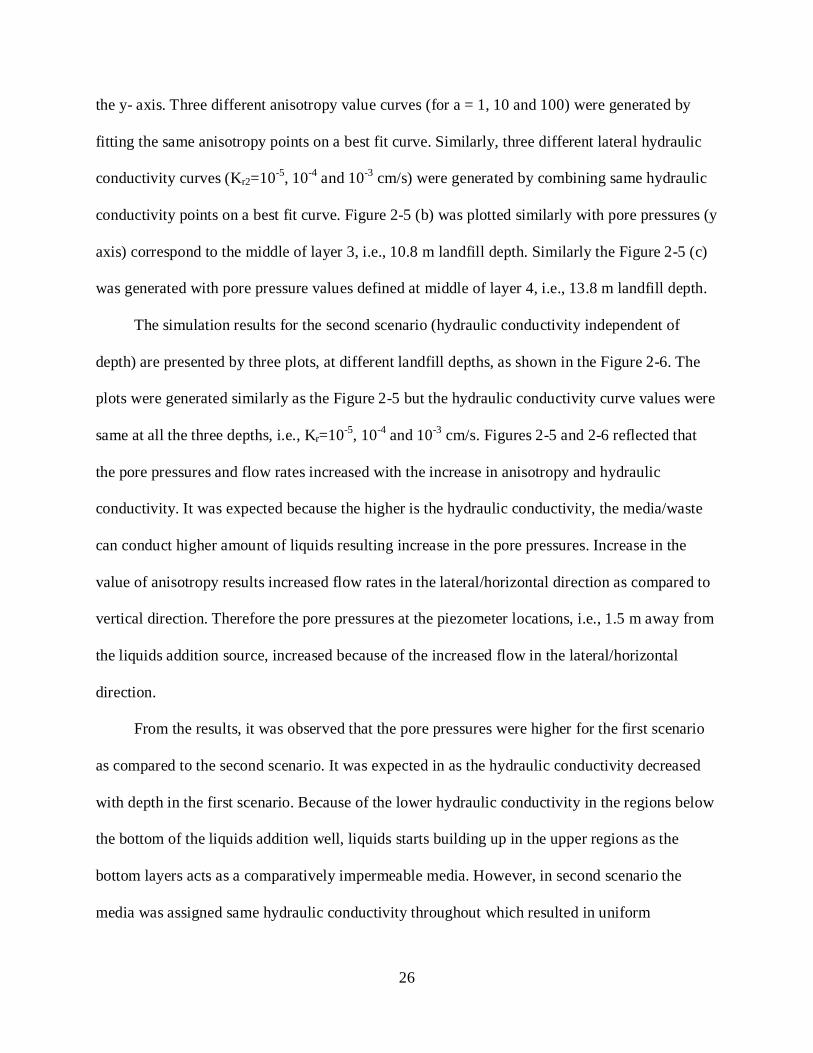
26

the y- axis. Three different anisotropy value curves (for a = 1, 10 and 100) were generated by

fitting the same anisotropy points on a best fit curve. Similarly, three different lateral hydraulic

conductivity curves (Kr2=10-5, 10-4 and 10-3 cm/s) were generated by combining same hydraulic

conductivity points on a best fit curve. Figure 2-5 (b) was plotted similarly with pore pressures (y

axis) correspond to the middle of layer 3, i.e., 10.8 m landfill depth. Similarly the Figure 2-5 (c)

was generated with pore pressure values defined at middle of layer 4, i.e., 13.8 m landfill depth.

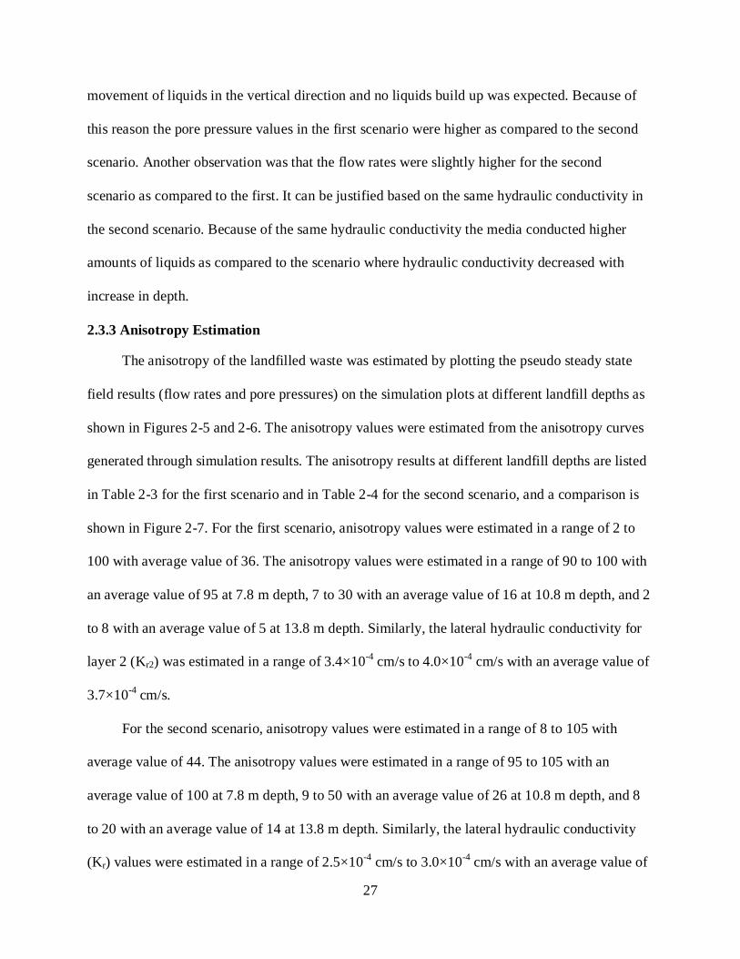
The simulation results for the second scenario (hydraulic conductivity independent of

depth) are presented by three plots, at different landfill depths, as shown in the Figure 2-6. The

plots were generated similarly as the Figure 2-5 but the hydraulic conductivity curve values were

same at all the three depths, i.e., Kr=10-5, 10-4 and 10-3 cm/s. Figures 2-5 and 2-6 reflected that

the pore pressures and flow rates increased with the increase in anisotropy and hydraulic

conductivity. It was expected because the higher is the hydraulic conductivity, the media/waste

can conduct higher amount of liquids resulting increase in the pore pressures. Increase in the

value of anisotropy results increased flow rates in the lateral/horizontal direction as compared to

vertical direction. Therefore the pore pressures at the piezometer locations, i.e., 1.5 m away from

the liquids addition source, increased because of the increased flow in the lateral/horizontal

direction.

From the results, it was observed that the pore pressures were higher for the first scenario

as compared to the second scenario. It was expected in as the hydraulic conductivity decreased

with depth in the first scenario. Because of the lower hydraulic conductivity in the regions below

the bottom of the liquids addition well, liquids starts building up in the upper regions as the

bottom layers acts as a comparatively impermeable media. However, in second scenario the

media was assigned same hydraulic conductivity throughout which resulted in uniform

27

movement of liquids in the vertical direction and no liquids build up was expected. Because of

this reason the pore pressure values in the first scenario were higher as compared to the second

scenario. Another observation was that the flow rates were slightly higher for the second

scenario as compared to the first. It can be justified based on the same hydraulic conductivity in

the second scenario. Because of the same hydraulic conductivity the media conducted higher

amounts of liquids as compared to the scenario where hydraulic conductivity decreased with

increase in depth.

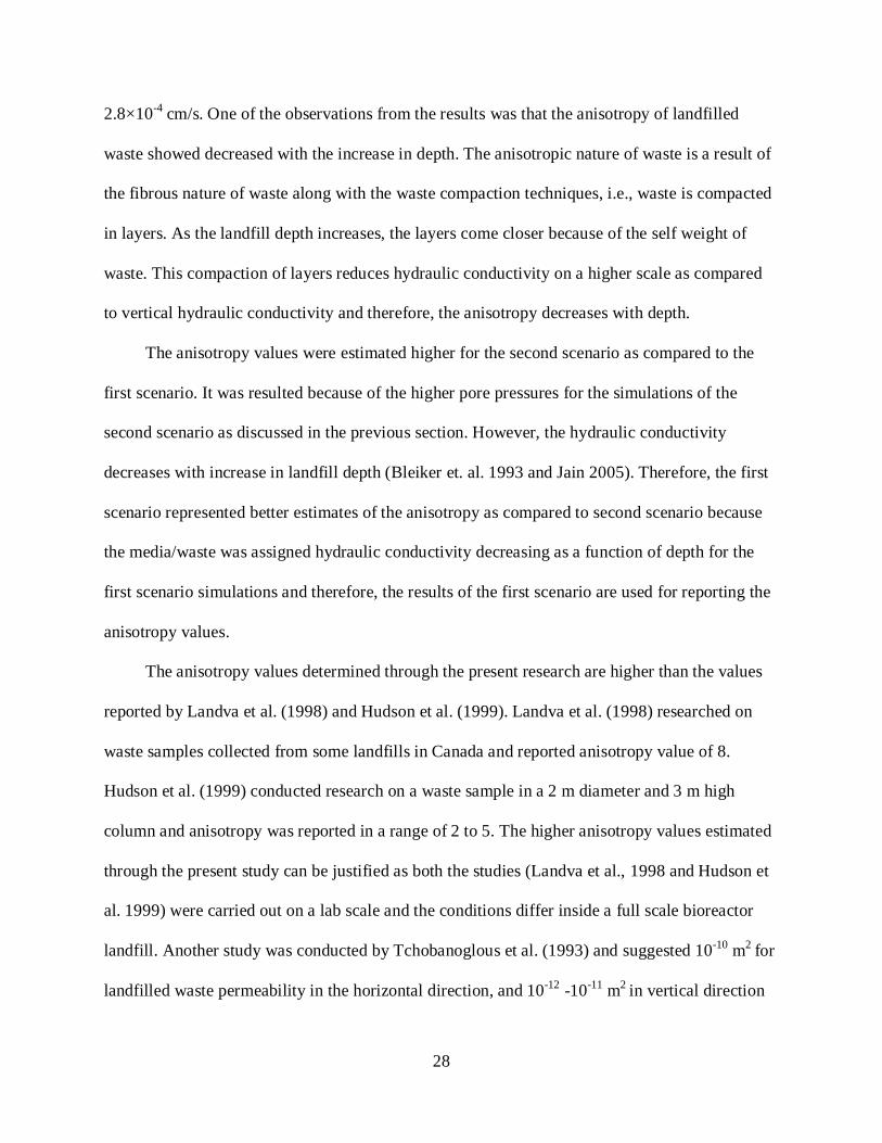
2.3.3 Anisotropy Estimation

The anisotropy of the landfilled waste was estimated by plotting the pseudo steady state

field results (flow rates and pore pressures) on the simulation plots at different landfill depths as

shown in Figures 2-5 and 2-6. The anisotropy values were estimated from the anisotropy curves

generated through simulation results. The anisotropy results at different landfill depths are listed

in Table 2-3 for the first scenario and in Table 2-4 for the second scenario, and a comparison is

shown in Figure 2-7. For the first scenario, anisotropy values were estimated in a range of 2 to

100 with average value of 36. The anisotropy values were estimated in a range of 90 to 100 with

an average value of 95 at 7.8 m depth, 7 to 30 with an average value of 16 at 10.8 m depth, and 2

to 8 with an average value of 5 at 13.8 m depth. Similarly, the lateral hydraulic conductivity for

layer 2 (Kr2) was estimated in a range of 3.4×10-4 cm/s to 4.0×10-4 cm/s with an average value of

3.7×10-4 cm/s.

For the second scenario, anisotropy values were estimated in a range of 8 to 105 with

average value of 44. The anisotropy values were estimated in a range of 95 to 105 with an

average value of 100 at 7.8 m depth, 9 to 50 with an average value of 26 at 10.8 m depth, and 8

to 20 with an average value of 14 at 13.8 m depth. Similarly, the lateral hydraulic conductivity

(Kr) values were estimated in a range of 2.5×10-4 cm/s to 3.0×10-4 cm/s with an average value of

28

2.8×10-4 cm/s. One of the observations from the results was that the anisotropy of landfilled

waste showed decreased with the increase in depth. The anisotropic nature of waste is a result of

the fibrous nature of waste along with the waste compaction techniques, i.e., waste is compacted

in layers. As the landfill depth increases, the layers come closer because of the self weight of

waste. This compaction of layers reduces hydraulic conductivity on a higher scale as compared

to vertical hydraulic conductivity and therefore, the anisotropy decreases with depth.

The anisotropy values were estimated higher for the second scenario as compared to the

first scenario. It was resulted because of the higher pore pressures for the simulations of the

second scenario as discussed in the previous section. However, the hydraulic conductivity

decreases with increase in landfill depth (Bleiker et. al. 1993 and Jain 2005). Therefore, the first

scenario represented better estimates of the anisotropy as compared to second scenario because

the media/waste was assigned hydraulic conductivity decreasing as a function of depth for the

first scenario simulations and therefore, the results of the first scenario are used for reporting the

anisotropy values.

The anisotropy values determined through the present research are higher than the values

reported by Landva et al. (1998) and Hudson et al. (1999). Landva et al. (1998) researched on

waste samples collected from some landfills in Canada and reported anisotropy value of 8.

Hudson et al. (1999) conducted research on a waste sample in a 2 m diameter and 3 m high

column and anisotropy was reported in a range of 2 to 5. The higher anisotropy values estimated

through the present study can be justified as both the studies (Landva et al., 1998 and Hudson et

al. 1999) were carried out on a lab scale and the conditions differ inside a full scale bioreactor

landfill. Another study was conducted by Tchobanoglous et al. (1993) and suggested 10-10 m2 for

landfilled waste permeability in the horizontal direction, and 10-12 -10-11 m2 in vertical direction

29

but the source did not reported any anisotropy values. Based on the suggested permeability

values, the anisotropy ratio is expected to be in a range of 10 to 100, and the average anisotropy

value determined through the present research is also found in the expected range.

The hydraulic conductivity of landfilled waste at 7.8 m depth was estimated in the range of

3.4×10-4 cm/s to 4.0×10-4 cm/s. In the previous studies, the hydraulic conductivity values have

been reported in the range of 6.7×10-5 cm/s to 9.8×10-4 cm/s by Shank 1993; 10-5 cm/s to 10-3

cm/s by Gabr 1995; 2.9×10-4 cm/s to 2.9×10-3 cm/s by Jang et al., 2002; 5.4×10-6 cm/s to 6.1×10-

5 cm/s Jain 2005; 1.2×10-2 cm/s to 6.9×10-2 cm/s by Koerner et al., 2005; and 1.2×10-4 cm/s to

1.2×10-2 cm/s by Durmusoglu 2006. Therefore the estimated values of the hydraulic conductivity

falls in the range of the reported values of the hydraulic conductivity of landfilled MSW.

2.3.4 Verification of Results

For modeling purposes the waste was assumed to be homogeneous media but the landfilled

waste is heterogeneous in nature because the municipal solid waste consists of different sizes and

types of wastes. Also the landfill gas resistance was assumed zero for modeling purpose,

however, gas may significantly impact the liquid phase flow (Powrie et al. 2008). For the present

research, steady state was assumed near the end of liquids addition period whereas the simulations

results were the steady state results. Because of these limitations and assumptions, the model

results would not truly match field results but rather provides some estimates to determine

anisotropy of landfilled waste.

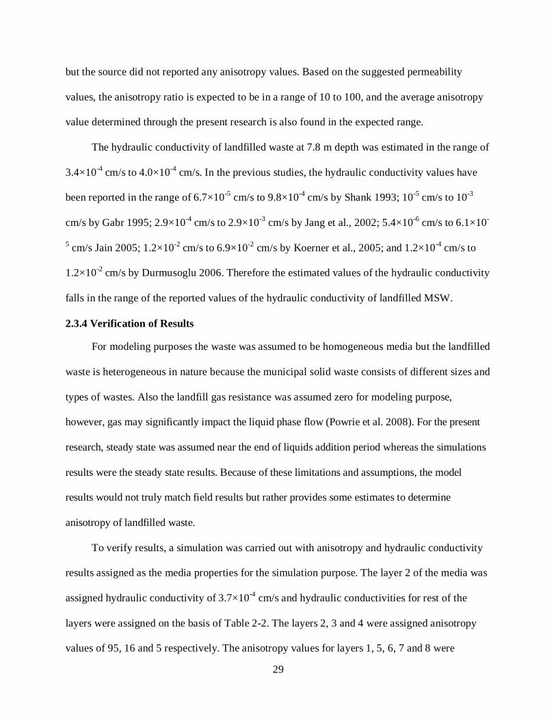
To verify results, a simulation was carried out with anisotropy and hydraulic conductivity

results assigned as the media properties for the simulation purpose. The layer 2 of the media was

assigned hydraulic conductivity of 3.7×10-4 cm/s and hydraulic conductivities for rest of the

layers were assigned on the basis of Table 2-2. The layers 2, 3 and 4 were assigned anisotropy

values of 95, 16 and 5 respectively. The anisotropy values for layers 1, 5, 6, 7 and 8 were

30

assumed as 95, 3, 2, 1 and 1 respectively. All other conditions were kept similar to the conditions

of first scenario simulations. The simulation results were plotted by taking pore pressures along

y-axis and landfill depth along x-axis as shown in Figure 2-8. The field data points were plotted

on the plot generated through simulation results. The field data points lay on the curve which

showed that the modeling results (used as input parameters for the last simulation) represented

the best set of anisotropy and hydraulic conductivity values for the different layers of the

simulated media.

2.4 Conclusions

This study reports the values of anisotropy of landfilled MSW by comparing field results

of liquids addition with simulation results. The anisotropy value was estimated in a range of 2 to

100 and decreased with increase in landfill depth with an average value of 36. The anisotropy

value was reported in a range of 2 to 8 by Landva et al. (1998) and Hudson et al. (1999).

Therefore, the average anisotropy value is found higher than the values reported by the previous

studies. This can be justified as both the studies were carried out at a lab scale and the conditions

differ inside a full scale bioreactor landfill. The radial and vertical impact zones, created due to

liquids addition, are closely associated with the anisotropy values associated with landfilled

MSW. The higher is the anisotropy value, the longer will be the radial impact zone. In a

subsurface moisture addition system the spacing between vertical wells or horizontal injection

lines is based upon radial and vertical impact zones created by moisture addition. The spacing

between liquids addition vertical wells and/or horizontal lines is a critical parameter to know

because if it is shorter than the optimum value then the associated cost increases and if it is

longer than the optimum value than there will be dry areas in between vertical wells and/or

horizontal lines. Therefore, the anisotropy values estimated through this study will help landfill

designers to design effective liquids addition system by calculating optimum spacing. The

31

associated lateral hydraulic conductivity was found in a range of 3.4×10-4 cm/s to 4.0×10-4 cm/s

with an average value of 3.7×10-4 cm/s. The value falls in the range of hydraulic conductivities

reported by previous studies.

32

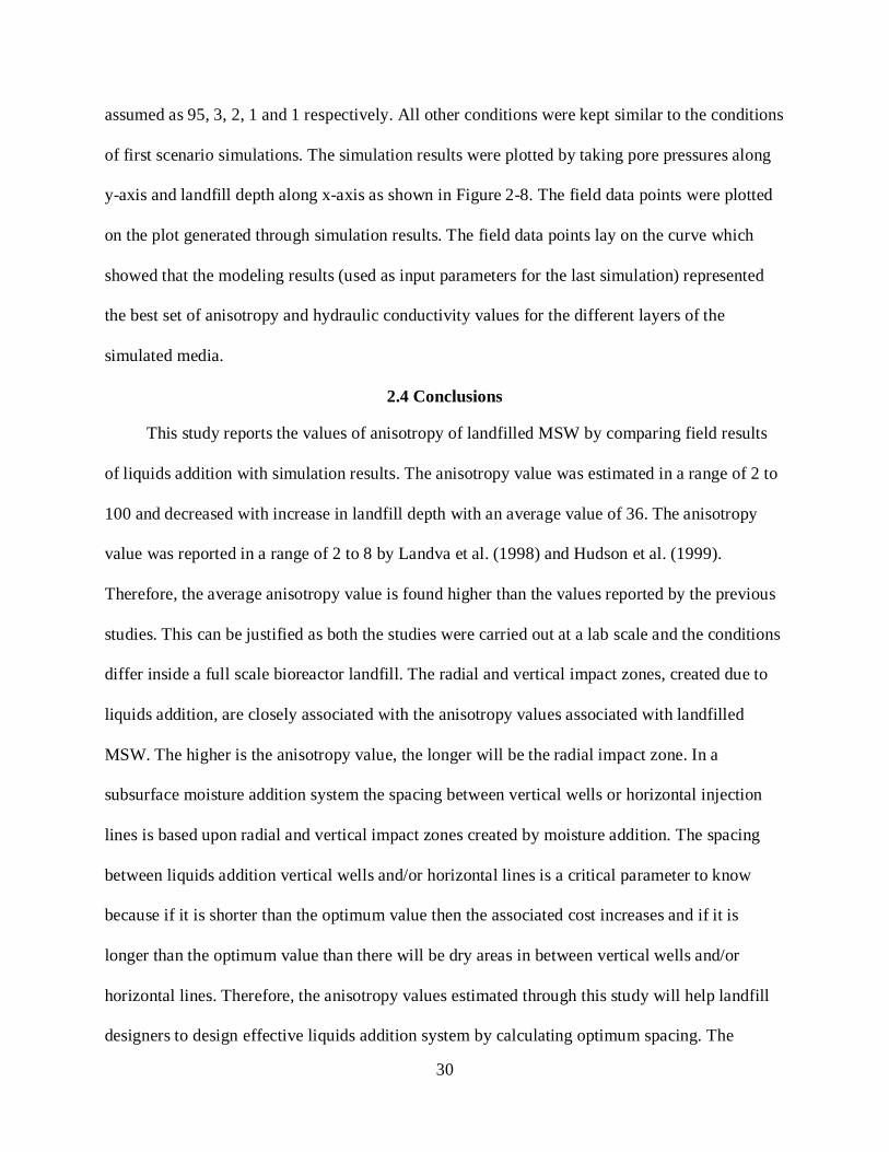
Table 2-1. Parameters used for the numerical modeling Parameter Value Hydraulic Conductivity for layer 2 (Kr2) (cms-1) 10-3, 10-4 and10-5 Anisotropy Ratio 1, 10 and 100 Van Genuchten parameter, a 1 (m-1of water column) Van Genuchten parameter, n 4 Van Genuchten parameter, m 0.75 Porosity (Vol/Vol) a 0.50 Waste Compressibility, αm (KPa-1) 3×10-3 Landfill Depth, (m) 50 Well Radius (m) 0.3 Well Depth (m) 12 Screen Length (m) 10.5 Injection Pressure (m) 16.4 a 50% porosity is assumed on the basis of the porosity range (45.5% to 55.5%) determined by Hudson et. al. (2004). Table 2-2. Hydraulic conductivity of different layers with respect to layer 2 Layer Average

Depth (m) Hydraulic Conductivity (m/s) a

Lateral Hydraulic Conductivity w.r.t. layer 2 b

1 3.2 8.9×10-5 1.25 × Kr2 2 7.8 7.1×10-5 Kr2 3 10.8 6.0×10-5 Kr2 / 1.18 4 13.8 4.7×10-5 Kr2 / 1.51 5 16.8 3.5×10-5 Kr2 / 2.03 6 19.8 2.5×10-5 Kr2 / 2.84 7 25.7 6.5×10-6 Kr2 / 10.92 8 40.0 5.0×10-7 Kr2 / 178 a Vertical hydraulic conductivity, calculated on basis of hydraulic conductivity as a function of depth of landfilled waste plot by Powrie and Beaven (1999). b The vertical hyd. conductivity ratio at two different depths will be equal to the ratio of lateral hyd. conductivity as all the layers have same anisotropy.

33

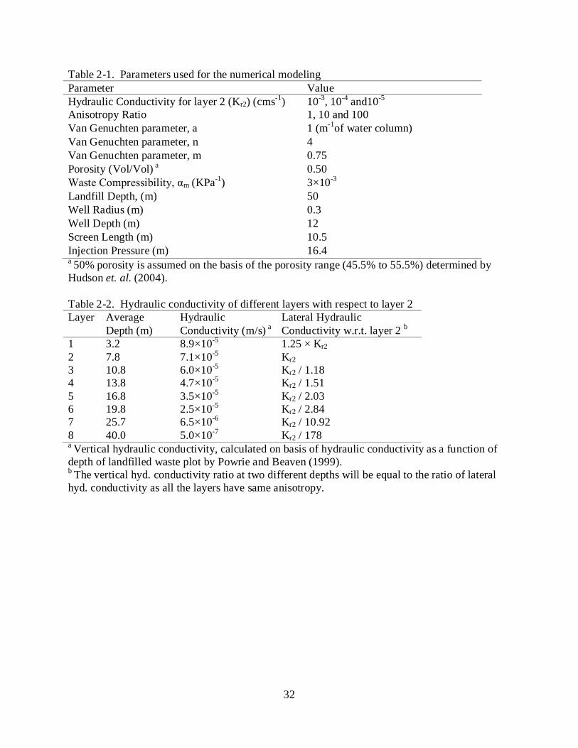
Table 2-3. Comparison of field data and simulation data for the first scenario Piezometer Well

Depth of Piezometer Inside Landfill (m)

Steady State Pore Pressure, m water column (field data)a

Anisotropy (comparing field data with simulation data)b

Hydraulic Conductivity, Kr2 (comparing field data with simulation data)b

C 7.8 3.9 100 4.0×10-4 cm/s J 7.8 3.8 90 4.0×10-4 cm/s C 10.8 4.4 10 3.7×10-4 cm/s G 10.8 4.1 7 3.5×10-4 cm/s J 10.8 4.7 30 4.0×10-4 cm/s C 13.8 5.2 2 3.6×10-4 cm/s G 13.8 5.8 8 3.4×10-4 cm/s a From Figure 2-4. b Calculated by overlapping steady state flow rate and steady state pore pressure (at piezometer locations; Figure 2-4) with the simulation results (Figure 2-5). Table 2-4. Comparison of field data and simulation data for the second scenario Piezometer Well

Depth of Piezometer Inside Landfill (m)

Steady State Pore Pressure, m water column (field data)a

Anisotropy (comparing field data with simulation data)b

Hydraulic Conductivity, Kr (comparing field data with simulation data)b

C 7.8 3.9 105 3.0×10-4 cm/s J 7.8 3.8 95 3.0×10-4 cm/s C 10.8 4.4 20 2.7×10-4 cm/s G 10.8 4.1 9 2.5×10-4 cm/s J 10.8 4.7 50 3.0×10-4 cm/s C 13.8 5.2 8 2.7×10-4 cm/s G 13.8 5.8 20 2.5×10-4 cm/s a From Figure 2-4. b Calculated by overlapping steady state flow rate and steady state pore pressure (at piezometer locations; Figure 2-4) with the simulation results (Figure 2-6).

34

A B Figure 2-1. A) New River Regional Landfill (NRRL) showing the area which contains the

moisture addition and the piezometer wells; B) the close up of the liquids addition wells and piezometer wells in the research area

35

Figure 2-2. Cross Sectional View of the liquids addition wells and the piezometer wells

36

Figure 2-3. Simulated landfill showing different layers of the media/waste

37

Pore

Pre

ssur

e (m

wat

er c

olum

n)

1

2

3

4

5

6

Piezometer located in Piezometer Well "C"Piezometer located in Piezometer Well "J"

Pore

Pre

ssur

e (m

wat

er c

olum

n)1

2

3

4

5

6Piezometer located in Peizometer Well "C" Piezometer located in Piezometer Well "G"Piezometer located in Piezometer Well "J"

Days (Day 1: Feb 5, 2010)0 2 4 6 8 10 12 14

Pore

Pre

ssur

e (m

wat

er c

olum

n)

2

3

4

5

6

Peizometer located in Piezometer Well "C" Peizometer located in Piezometer Well "G"

B

A

C

Figure 2-4. Pore Pressure Vs Time for the piezometers located at A) 7.8m depth; B) 10.8 m depth; C) 13.8 m depth; (from field data)

38

Pore

Pre

ssur

e (m

)

0

2

4

6

8Anisotropy=1Anisotropy= 10Anisotropy= 100

Kr2 = 10-5 cm/s

Well "C" Piezometer (Field Data Point)Well "J" Piezometer (Field Data Point)

Kr2 = 10-4 cm/s Kr2 = 10-3 cm/sPo

re P

ress

ure

(m)

0

2

4

6

8Anisotropy=1Anisotropy= 10Anisotropy= 100

Kr2 = 10-4 cm/sKr2 = 10-3 cm/s

Kr2 = 10-5 cm/s

Well "C" Piezometer (Field Data Point)Well "J" Piezometer (Field Data Point)Well "G" Piezometer (Field Data Point)

Flowrate (m3/s)1e-6 1e-5 1e-4 1e-3 1e-2

Pore

Pre

ssur

e (m

)

0

2

4

6

8

Anisotropy=1Anisotropy= 10Anisotropy= 100Well "C" Piezometer (Field Data Point)

Well "G" Piezometer (Field Data Point)

Kr2 = 10-5 cm/s

Kr2 = 10-4 cm/sKr2 = 10-3 cm/s

A

B

C

Figure 2-5. Plots generated through modeling results for first scenario A) at landfill depth of 7.8 m; B) at landfill depth of 10.8 m; and C) at landfill depth of 13.8 m. The plots also include field data points

39

Pore

Pre

ssur

e (m

)

0

2

4

6

8Anisotropy=1Anisotropy= 10Anisotropy= 100

Well "C" Piezometer (Field Data Point)Well "J" Piezometer (Field Data Point)

Kr = 10-5 cm/sKr = 10-4 cm/s Kr = 10-3 cm/s

Pore

Pre

ssur

e (m

)

0

2

4

6

8Anisotropy=1Anisotropy= 10Anisotropy= 100

Kr = 10-5 cm/s

Well "C" Piezometer (Field Data Point)Well "J" Piezometer (Field Data Point)Well "G" Piezometer (Field Data Point)

Kr = 10-4 cm/s Kr = 10-3 cm/s

Flowrate (m3/s)1e-6 1e-5 1e-4 1e-3 1e-2

Pore

Pre

ssur

e (m

)

0

2

4

6

8

Anisotropy=1Anisotropy= 10Anisotropy= 100Well "C" Piezometer (Field Data Point)

Well "G" Piezometer (Field Data Point)

Kr = 10-5 cm/s

Kr = 10-4 cm/s Kr = 10-3 cm/s

A

B

C

Figure 2-6. Plots generated through modeling results for second scenario A) at landfill depth of

7.8 m; B) at landfill depth of 10.8 m; and C) at landfill depth of 13.8 m. The plots also include field data points

40

Landfill Depth (m)

7 8 9 10 11 12 13 14 15

Anis

otro

py

0

20

40

60

80

100 Mean Value (Scenario 1)Mean Value (Scenario 2)

Figure 2-7. Comparison of anisotropy results for two different scenarios

41

Landfill Depth (m)

7 8 9 10 11 12 13 14 15

Pore

Pre

ssur

e (m

wat

er c

olum

n)

0

1

2

3

4

5

6

Field DataSimulation Results

Figure 2-8. Comparison of pore pressures field results with results of the simulation carried out for the verification of results

42

CHAPTER 3 PERFORMANCE EVALUATION OF SURFACE INFILTRATION TRENCHES WITH

WHOLE TIRES AS A BEDDING MEDIA

3.1 Introduction

Liquids addition is the most important tool for bioreacting landfilled waste. Surface and

subsurface liquids addition systems are two of the most commonly practiced systems. Horizontal

injection lines and vertical wells are two examples of subsurface liquids additions systems and

considerable research has been conducted on various aspects of these systems (McCreanor et al.

1996 and 2000, Townsend et al. 1998, McCreanor 1998, Haydar et al. 2004 and 2005, Jain 2005,

Larson 2007, Kadambala 2009). Surface infiltration ponds and surface infiltration trenches are

two types of surface liquids addition systems; Townsend et al. (1995) reported results from

surface infiltration ponds but after this study, little research has been conducted on surface

infiltration systems.

Townsend et al. (1995) conducted research on four surface infiltration ponds and operated

the system for 28-month period. The performances of the infiltration ponds were reported in

terms of the infiltration rates, defined as flow rate per unit wetted bottom area. The infiltration

rates were reported in a rage of 6.0×10-8 m/s to 9.0×10-8 m/s. Larson (2007) researched on 16

subsurface horizontal injection lines (HILs) with different bedding materials around the

perforated pipe. The performance the HILs was reported in terms of fluid conductance, defined

as pseudo steady state flow rate per unit applied pressure per unit length. The performances of

HILs were reported in a range of 1.9×10-7 m/s to 7.5×10-7 m/s with an average of 5.3×10-7 m/s.

Kumar (2009) researched on 31 HILs with different bedding materials and reported fluid

conductance values in a range of 1.6×10-7 m/s to 3.4×10-6 m/s with an average of 7.8×10-7 m/s.

This study aims to continue and build upon these past studies by examining the performance of

43

surface infiltration trenches (SITs) and comparing the results with these studies on surface and

subsurface liquids addition systems.

Another aspect of this research is to provide an innovative way to use whole scrap tires a

bedding material. The management of whole scrap tires is a challenge in solid waste

management field. Approximately 290 million scrap tires are generated annually and

approximately 275 million scrap tires were present in stockpiles in 2003. The stockpiled tires

pose threat to the environment because of fire breakouts and vectors. Tire fires typically cause

air, surface water, soil, groundwater, and residual contamination. Scrap tires are managed by

using tires as fuel for incinerators, and land application besides stockpiling. Another option for

the management of scrap tires is to use shredded tires as a bedding material and this option has

been practiced at some operating landfills (Larson 1997, Kumar 2009). However, processing is

required for the shredded tires and thus, the use of whole tires provides an economical and

environmental benefit.

3.2 Materials and Methods

3.2.1 Site Description

The research was carried out in Cell 5 at the New River Regional Landfill (NRRL) located

in Union County, Florida. The NRRL receives 800 metric tons per day of waste consisting of

mixed residential and commercial waste. The landfill currently consists of five class-I

contiguous lined landfill cells totaling approximately 25 hectares. Cell 5 is approximately 6.9

hectares in area and is equipped with a double liner system. The average height of the waste from

the surface of the landfill to the leachate collection system at the time of construction was

approximately 13 m. The density of the landfilled waste was approximated to be 710 kg/m3. A

clayey-sandy soil mined on site was used as daily cover. Leachate recirculation was permitted in

Cell 5 at the time of operation; however the maximum amount of leachate recirculated should

44

not have exceeded a total volume 122 m3 per day. A detailed description of the site and the

bioreactor can be found elsewhere (Jain 2005 and Kadambala 2009).

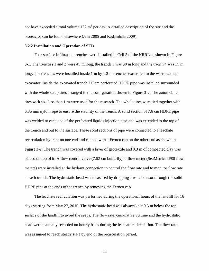
3.2.2 Installation and Operation of SITs

Four surface infiltration trenches were installed in Cell 5 of the NRRL as shown in Figure

3-1. The trenches 1 and 2 were 45 m long, the trench 3 was 30 m long and the trench 4 was 15 m

long. The trenches were installed inside 1 m by 1.2 m trenches excavated in the waste with an

excavator. Inside the excavated trench 7.6 cm perforated HDPE pipe was installed surrounded

with the whole scrap tires arranged in the configuration shown in Figure 3-2. The automobile

tires with size less than 1 m were used for the research. The whole tires were tied together with

6.35 mm nylon rope to ensure the stability of the trench. A solid section of 7.6 cm HDPE pipe

was welded to each end of the perforated liquids injection pipe and was extended to the top of

the trench and out to the surface. These solid sections of pipe were connected to a leachate

recirculation hydrant on one end and capped with a Fernco cap on the other end as shown in

Figure 3-2. The trench was covered with a layer of geotextile and 0.3 m of compacted clay was

placed on top of it. A flow control valve (7.62 cm butterfly), a flow meter (SeaMetrics IP80 flow

meters) were installed at the hydrant connection to control the flow rate and to monitor flow rate

at each trench. The hydrostatic head was measured by dropping a water sensor through the solid

HDPE pipe at the ends of the trench by removing the Fernco cap.

The leachate recirculation was performed during the operational hours of the landfill for 16

days starting from May 27, 2010. The hydrostatic head was always kept 0.3 m below the top

surface of the landfill to avoid the seeps. The flow rate, cumulative volume and the hydrostatic

head were manually recorded on hourly basis during the leachate recirculation. The flow rate

was assumed to reach steady state by end of the recirculation period.

45

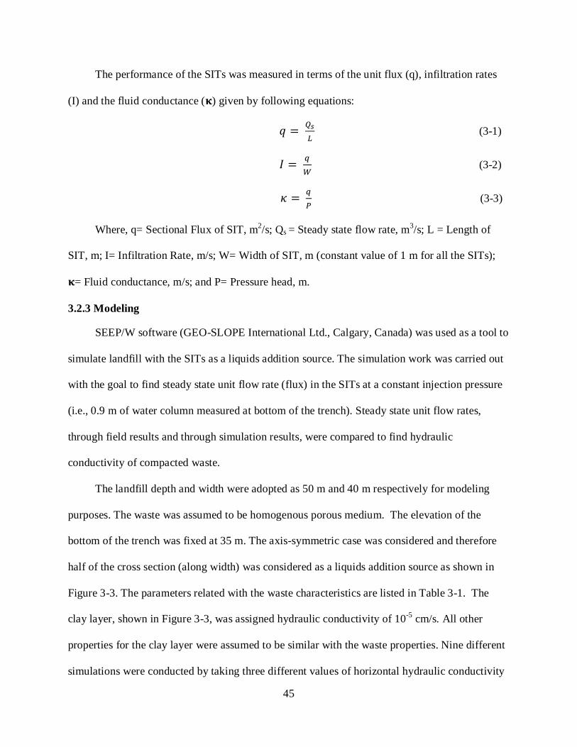
The performance of the SITs was measured in terms of the unit flux (q), infiltration rates

(I) and the fluid conductance (𝛋) given by following equations:

𝑞 = 𝑄𝑠𝐿

(3-1)

𝐼 = 𝑞𝑊

(3-2)

𝜅 = 𝑞𝑃 (3-3)

Where, q= Sectional Flux of SIT, m2/s; Qs = Steady state flow rate, m3/s; L = Length of

SIT, m; I= Infiltration Rate, m/s; W= Width of SIT, m (constant value of 1 m for all the SITs);

𝛋= Fluid conductance, m/s; and P= Pressure head, m.

3.2.3 Modeling

SEEP/W software (GEO-SLOPE International Ltd., Calgary, Canada) was used as a tool to

simulate landfill with the SITs as a liquids addition source. The simulation work was carried out

with the goal to find steady state unit flow rate (flux) in the SITs at a constant injection pressure

(i.e., 0.9 m of water column measured at bottom of the trench). Steady state unit flow rates,

through field results and through simulation results, were compared to find hydraulic

conductivity of compacted waste.

The landfill depth and width were adopted as 50 m and 40 m respectively for modeling

purposes. The waste was assumed to be homogenous porous medium. The elevation of the

bottom of the trench was fixed at 35 m. The axis-symmetric case was considered and therefore

half of the cross section (along width) was considered as a liquids addition source as shown in

Figure 3-3. The parameters related with the waste characteristics are listed in Table 3-1. The

clay layer, shown in Figure 3-3, was assigned hydraulic conductivity of 10-5 cm/s. All other

properties for the clay layer were assumed to be similar with the waste properties. Nine different

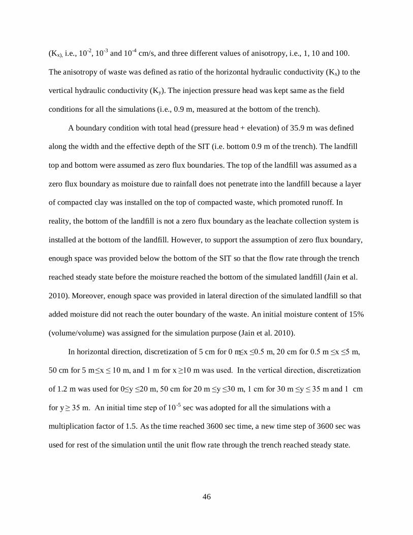
simulations were conducted by taking three different values of horizontal hydraulic conductivity

46

(Kx), i.e., 10-2, 10-3 and 10-4 cm/s, and three different values of anisotropy, i.e., 1, 10 and 100.

The anisotropy of waste was defined as ratio of the horizontal hydraulic conductivity (Kx) to the

vertical hydraulic conductivity (Ky). The injection pressure head was kept same as the field

conditions for all the simulations (i.e., 0.9 m, measured at the bottom of the trench).

A boundary condition with total head (pressure head + elevation) of 35.9 m was defined

along the width and the effective depth of the SIT (i.e. bottom 0.9 m of the trench). The landfill

top and bottom were assumed as zero flux boundaries. The top of the landfill was assumed as a

zero flux boundary as moisture due to rainfall does not penetrate into the landfill because a layer

of compacted clay was installed on the top of compacted waste, which promoted runoff. In

reality, the bottom of the landfill is not a zero flux boundary as the leachate collection system is

installed at the bottom of the landfill. However, to support the assumption of zero flux boundary,

enough space was provided below the bottom of the SIT so that the flow rate through the trench

reached steady state before the moisture reached the bottom of the simulated landfill (Jain et al.

2010). Moreover, enough space was provided in lateral direction of the simulated landfill so that

added moisture did not reach the outer boundary of the waste. An initial moisture content of 15%

(volume/volume) was assigned for the simulation purpose (Jain et al. 2010).

In horizontal direction, discretization of 5 cm for 0 m ≤x ≤0.5 m, 20 cm for 0.5 m ≤x ≤5 m,

50 cm for 5 m ≤x ≤ 10 m, and 1 m for x ≥10 m was used. In the vertical direction, discretization

of 1.2 m was used for 0 ≤y ≤20 m, 50 cm for 20 m ≤y ≤30 m, 1 cm for 30 m ≤y ≤ 35 m and 1 cm

for y ≥ 35 m. An initial time step of 10 -5 sec was adopted for all the simulations with a

multiplication factor of 1.5. As the time reached 3600 sec time, a new time step of 3600 sec was

used for rest of the simulation until the unit flow rate through the trench reached steady state.

47

3.2.4 Hydraulic Conductivity Estimation

The simulation results were plotted by taking hydraulic conductivity values along the x-

axis and steady state flux along y-axis for nine different simulations. The points with the same

anisotropy value were fitted on a best fit curve and therefore, the plot represented three different

anisotropy value curves. The observed pseudo steady state flux values (from field data) were

plotted on the simulation plot to estimate the hydraulic conductivity of the landfilled waste.

3.2.5 Model Limitations

For the modeling purpose the waste was assumed to be homogeneous media but the

landfilled waste is heterogeneous in nature. Also the landfill gas resistance was assumed zero for

modeling purpose, however, gas may significantly impact the liquid phase flow (Powrie et al.

2008). The model simulated the scenario where liquids addition system was operated on a

continuous basis; however, the SITs were operated on an intermittent basis. Because of these

limitations and assumptions, the model results would not truly match field results but rather

provides some close estimates to determine hydraulic conductivity of landfilled waste.

3.3 Results and Discussion

3.3.1 Performance of SITs

The leachate recirculation was performed for 16 days and approximately 365 m3 of liquids

were added into the four SITs. Figures 3-4 and 3-5 show the change of flux and pressure head for

the four SITs with respect to time and cumulative volume. The pressure increased in the earlier

stage of liquids addition and it was kept constant in the later stage of the experiment by adjusting

the flow control valve. The sectional flux was higher in the earlier stage of liquids addition and it

decreased continuously during the remaining period of liquids addition. However the flux values

did not change significantly near the end of liquids addition and therefore, the sectional flux

values were assumed to reach pseudo steady state at the end of liquids addition. The pseudo

48

steady state sectional flux value for 15 m, 30 m, 45 m and the second 45 m trench was found

8.0×10-6 m2/s, 8.8×10-6 m2/s, 1.1×10-5 m2/s and 9.1×10-6 m2/s respectively. The magnitude of

pseudo steady state infiltration rates (I) remained as the sectional flux (q) because the width of all

four SITs was 1 m. The fluid conductance values were observed in a range of 8.9×10-6 m/s to

1.2×10-5 m/s with an average value of 1.0×10-5 m/s.

Townsend et al. (1995) reported infiltration rates ranged from 6.0×10-8 m/s to 9.0×10-8 m/s.

The surface infiltration rates, through the present research, were observed in a range of 8.0×10-6

m/s to 1.1×10-5 m/s which is 120 to 130 times higher than the values of infiltration rates reported

by Townsend et al. (1995). Therefore the performance of the SITs was observed better than the

performance of the infiltration ponds. Townsend et al. (1995) added approximately 3 m3/m2

(cumulative volume added/surface area of ponds) of liquids in a period of 140 to 385 days

whereas for the present research, 2.7 m3/m2 (cumulative volume added/surface areas of SITs) in

a period of 16 days. Therefore the SITs conducted approximately the same amount of liquids but

in smaller duration of time which supports the higher infiltration rates for the present research.

Townsend et al. (1995) researched at Alachua County SW Landfill (ACSWL) which was an old

landfill as compared to research site used for the present research (i.e., NRRL) and therefore, the

landfill waste for the ACSWL is expected to have higher density than the waste density of the

NRRL. Because of these differences, i.e., different liquids addition times and research sites, the

performance comparison is not accurate but only provides some close estimates.

Larson (2007) conducted research on 16 subsurface horizontal injection lines (HILs) and

fluid conductance values were reported in a range of 1.9×10-7 m/s to 7.5×10-7 m/s with an

average of 5.3×10-7 m/s. Kumar (2009) also researched on 31 HILs and fluid conductance values

were reported in a range of 1.6×10-7 m/s to 3.4×10-6 m/s with an average of 7.8×10-7 m/s.

49

Therefore, the average fluid conductance was observed 13 to 19 times higher than the values

reported values by Larson (2007) and Kumar (2009). This is justifiable because the hydraulic

conductivity is higher near the surface of the landfill and it decreases with depth (Bleiker et al.

1993, Powrie et al.1999 and Jain et al. 2006) and therefore, the surface liquids addition system

was expected to perform better than the subsurface liquids addition system.

3.3.2 Hydraulic Conductivity Estimation

The modeling results were plotted by taking hydraulic conductivity values along x-axis

and steady state sectional flux (q) values along y-axis for nine different simulations as shown in

Figure 3-6. Steady state flux decreased with the decrease in the hydraulic conductivity and vice-

versa. The hydraulic conductivity of waste decreases with the increase in density of landfilled

waste (Bleiker et. al. 1993). The void space, available for the movement of liquids, is reduced

with the increase in the density of landfilled waste, resulting in the reduced flux. Steady state

flux also show decrease with the increase in the anisotropy value, at a constant horizontal

hydraulic conductivity. The increase in the value of anisotropy results in the decrease of vertical

hydraulic conductivity, at constant horizontal hydraulic conductivity as anisotropy is defined as

Kx/Ky. Therefore, the decrease in the Ky results in the reduced flux.

Steady state flux values from the field data were plotted on the plot generated by modeling

results as shown in Figure 3-7. Assuming anisotropy value of waste ranging from 10 to 100

(based upon Chapter 2); the hydraulic conductivity was estimated at anisotropy values 10 and

100. The hydraulic conductivity values are listed in Table 3.2 separately for four SITs. The

average horizontal hydraulic conductivity value was found as 1.1×10-3 cm/s for anisotropy value

10 and 2.0×10-3 cm/s for anisotropy value 100; average vertical hydraulic conductivity value was

calculated as 1.1×10-4 cm/s for anisotropy value 10 and 2.0×10-5 cm/s for anisotropy value 100.

50

Townsend et al. 1995 calculated vertical hydraulic conductivity of 3.0×10-6 cm/s to 4.0×10-

6 cm/s. For the present research, the vertical hydraulic conductivity was estimated in a rage of

8.5×10-5 cm/s to 2.0×10-4 cm/s for anisotropy value of 10 and 1.4×10-5 cm/s to 3.7×10-5 cm/s for

anisotropy value of 100. The hydraulic conductivity at anisotropy value of 100 is more realistic

estimate as the anisotropy value is high near the top surface of the landfill. The estimated values

of hydraulic conductivity are observed higher than the values calculated by Townsend et al.

(1995). The difference of hydraulic conductivities between the two studies can be a result of the

different research sites and the modeling limitations.

3.3.3 Pros and Cons of SITs

The whole scrap tires proved to be a good bedding material because of the high infiltration

rates. During the research, tires did not create any surfacing problem (springing back of tires to

the top surface of the landfill), i.e., the problem due to which landfilling of whole tires is banned

in many states within the U.S.. It is not expected that tires will create the surfacing problem in

future as well because the tires were tied together which made it a heavy and stable single unit of

whole scrap tires. There are some economical benefits associated with the use of whole tires as a

bedding media because it is available for free. It costs approximately $13 to produce one cubic

meter shredded tires; the unit cost is based on the information provided by CM Tire Recycling,

Sarasota Florida. Therefore, the present research saved approximately $1,800 by preferring

whole scrap tires over shredded tires for a total SIT length of 135 m. Besides the economic

benefit the whole tires as bedding media is a better option as compared to shredded tires because

it reduces the fuel requirements and CO2 emissions which would have been caused by shredding

the whole scrap tires.

The SITs performed better than the infiltration ponds and one subsurface liquids addition

system (HILs). The SITs eliminated some problems associated with surface infiltration ponds

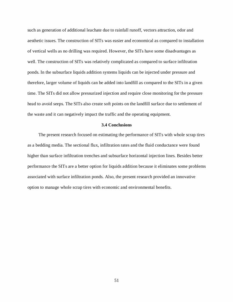
51

such as generation of additional leachate due to rainfall runoff, vectors attraction, odor and

aesthetic issues. The construction of SITs was easier and economical as compared to installation

of vertical wells as no drilling was required. However, the SITs have some disadvantages as

well. The construction of SITs was relatively complicated as compared to surface infiltration

ponds. In the subsurface liquids addition systems liquids can be injected under pressure and

therefore, larger volume of liquids can be added into landfill as compared to the SITs in a given

time. The SITs did not allow pressurized injection and require close monitoring for the pressure

head to avoid seeps. The SITs also create soft points on the landfill surface due to settlement of

the waste and it can negatively impact the traffic and the operating equipment.

3.4 Conclusions

The present research focused on estimating the performance of SITs with whole scrap tires

as a bedding media. The sectional flux, infiltration rates and the fluid conductance were found

higher than surface infiltration trenches and subsurface horizontal injection lines. Besides better

performance the SITs are a better option for liquids addition because it eliminates some problems

associated with surface infiltration ponds. Also, the present research provided an innovative

option to manage whole scrap tires with economic and environmental benefits.

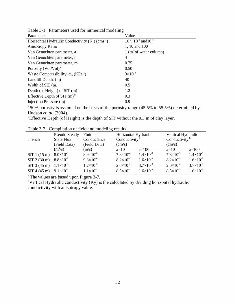
52

Table 3-1. Parameters used for numerical modeling Parameter Value Horizontal Hydraulic Conductivity (Kx) (cms-1) 10-2, 10-3 and10-4 Anisotropy Ratio 1, 10 and 100 Van Genuchten parameter, a 1 (m-1of water column) Van Genuchten parameter, n 4 Van Genuchten parameter, m 0.75 Porosity (Vol/Vol) a 0.50 Waste Compressibility, αm (KPa-1) 3×10-3 Landfill Depth, (m) 40 Width of SIT (m) 0.5 Depth (or Height) of SIT (m) 1.2 Effective Depth of SIT (m) b 0.3 Injection Pressure (m) 0.9 a 50% porosity is assumed on the basis of the porosity range (45.5% to 55.5%) determined by Hudson et. al. (2004). bEffective Depth (of Height) is the depth of SIT without the 0.3 m of clay layer. Table 3-2. Compilation of field and modeling results

Trench

Pseudo Steady State Flux (Field Data) (m2/s)

Fluid Conductance (Field Data) (m/s)

Horizontal Hydraulic Conductivity a (cm/s)

Vertical Hydraulic Conductivity b (cm/s)

a=10 a=100 a=10 a=100 SIT 1 (15 m) 8.0×10-6 8.9×10-6 7.8×10-4 1.4×10-3 7.8×10-5 1.4×10-5 SIT 2 (30 m) 8.8×10-6 9.8×10-6 8.2×10-4 1.6×10-3 8.2×10-5 1.6×10-5 SIT 3 (45 m) 1.1×10-5 1.2×10-5 2.0×10-3 3.7×10-3 2.0×10-4 3.7×10-5 SIT 4 (45 m) 9.1×10-6 1.1×10-5 8.5×10-4 1.6×10-3 8.5×10-5 1.6×10-5 a The values are based upon Figure 3-7. bVertical Hydraulic conductivity (Ky) is the calculated by dividing horizontal hydraulic conductivity with anisotropy value.

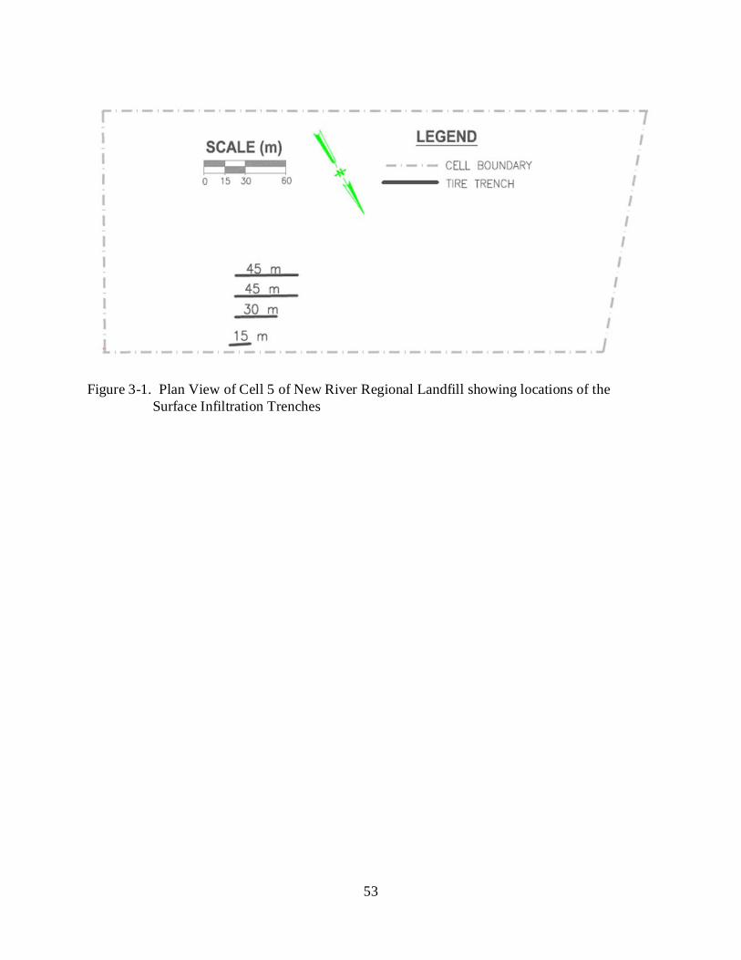
53

Figure 3-1. Plan View of Cell 5 of New River Regional Landfill showing locations of the

Surface Infiltration Trenches

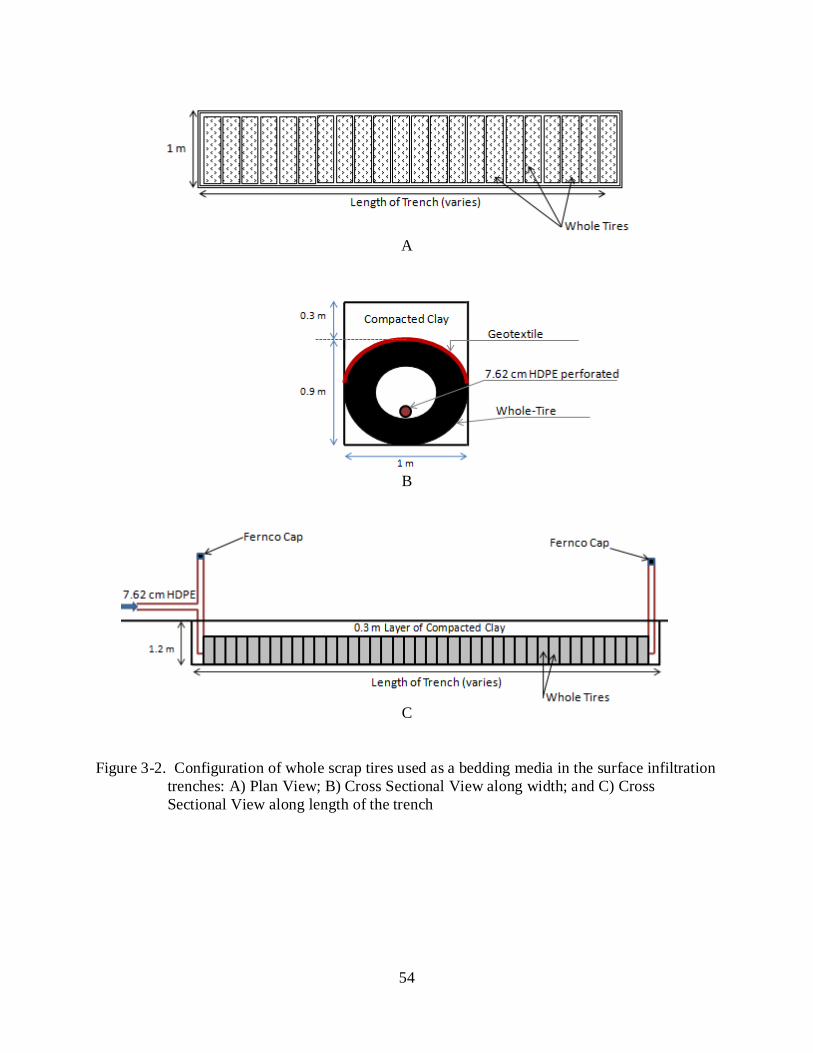
54

A

B

C

Figure 3-2. Configuration of whole scrap tires used as a bedding media in the surface infiltration trenches: A) Plan View; B) Cross Sectional View along width; and C) Cross Sectional View along length of the trench

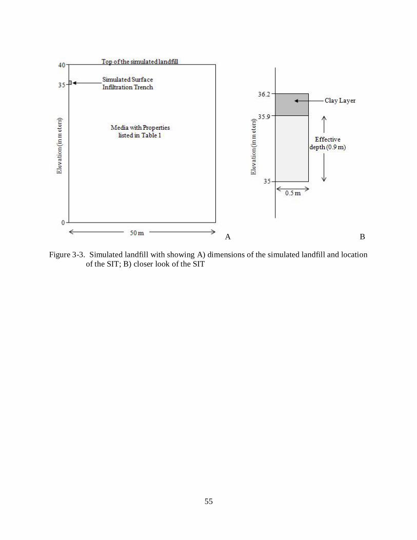
55

A B

Figure 3-3. Simulated landfill with showing A) dimensions of the simulated landfill and location of the SIT; B) closer look of the SIT

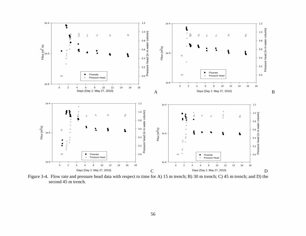
56

Days (Day 1: May 27, 2010)0 2 4 6 8 10 12 14 16 18

Fllu

x (m

/s)

1e-6

1e-5

1e-4

Pres

sure

hea

d (in

m w

ater

col

umn)

0.0

0.2

0.4

0.6

0.8

1.0

1.2

FlowratePressure Head

2

A Days (Day 1: May 27, 2010)

0 2 4 6 8 10 12 14 16 181e-6

1e-5

1e-4

0.0

0.2

0.4

0.6

0.8

1.0

1.2

FlowratePressure Head

Pres

sure

hea

d (in

m w

ater

col

umn)

Fllu

x (m

/s)

2

B

Days (Day 1: May 27, 2010)

0 2 4 6 8 10 12 14 16 181e-6

1e-5

1e-4

0.0

0.2

0.4

0.6

0.8

1.0

1.2

FlowratePressure Head

Pres

sure

hea

d (in

m w

ater

col

umn)

Fllu

x (m

/s)

2

C Days (Day 1: May 27, 2010)

0 2 4 6 8 10 12 14 16 181e-6

1e-5

1e-4

0.0

0.2

0.4

0.6

0.8

1.0

1.2

FlowratePressure Head

Pres

sure

hea

d (in

m w

ater

col

umn)

Fllu

x (m

/s)

2

D Figure 3-4. Flow rate and pressure head data with respect to time for A) 15 m trench; B) 30 m trench; C) 45 m trench; and D) the

second 45 m trench.

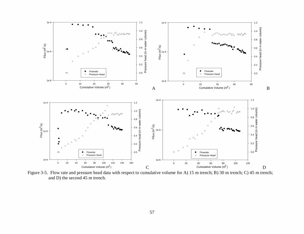
57

Cumulative Volume (m )0 10 20 30 40 50

Fllu

x (m

/s)

1e-6

1e-5

1e-4

Pres

sure

hea

d (in

m w

ater

col

umn)

0.0

0.2

0.4

0.6

0.8

1.0

1.2

FlowratePressure Head

2

3 A 0 20 40 60 80

1e-6

1e-5

1e-4

0.0

0.2

0.4

0.6

0.8

1.0

1.2

FlowratePressure Head

Pres

sure

hea

d (in

m w

ater

col

umn)

Cumulative Volume (m )3

Fllu

x (m

/s)

2

B

0 20 40 60 80 100 120 140 1601e-6

1e-5

1e-4

0.0

0.2

0.4

0.6

0.8

1.0

1.2

FlowratePressure Head

Pres

sure

hea

d (in

m w

ater

col

umn)

Cumulative Volume (m )3

Fllu

x (m

/s)

2

C 0 20 40 60 80 100 120

1e-6

1e-5

1e-4

0.0

0.2

0.4

0.6

0.8

1.0

1.2

FlowratePressure Head

Pres

sure

hea

d (in

m w

ater

col

umn)

Cumulative Volume (m )3

Fllu

x (m

/s)

2

D Figure 3-5. Flow rate and pressure head data with respect to cumulative volume for A) 15 m trench; B) 30 m trench; C) 45 m trench;

and D) the second 45 m trench.

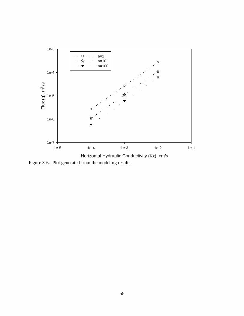
58

Horizontal Hydraulic Conductivity (Kx), cm/s

1e-5 1e-4 1e-3 1e-2 1e-1

Flux

(q),

m /

s

1e-7

1e-6

1e-5

1e-4

1e-3

a=1a=10a=100

2

Figure 3-6. Plot generated from the modeling results

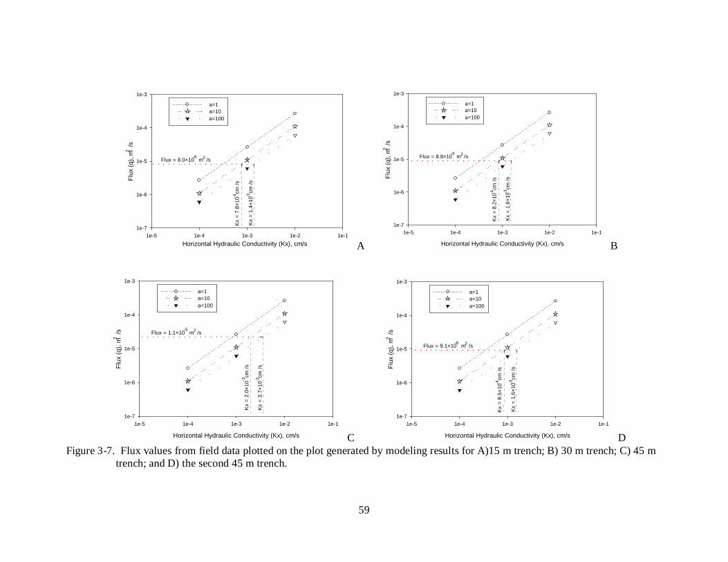
59

Horizontal Hydraulic Conductivity (Kx), cm/s1e-5 1e-4 1e-3 1e-2 1e-1

Flux

(q),

m /

s

1e-7

1e-6

1e-5

1e-4

1e-3

a=1a=10a=100

2

Flux = 8.0×10 m /s-6 2

Kx

= 7.

8×10

cm

/s-4

Kx

= 1.

4×10

cm

/s-3

A

Horizontal Hydraulic Conductivity (Kx), cm/s

1e-5 1e-4 1e-3 1e-2 1e-1

Flux

(q),

m /

s

1e-7

1e-6

1e-5

1e-4

1e-3

a=1a=10a=100

2

Flux = 8.8×10 m /s-6 2

Kx

= 8.

2×10

cm

/s-4

Kx

= 1.

6×10

cm

/s-3

B

Horizontal Hydraulic Conductivity (Kx), cm/s

1e-5 1e-4 1e-3 1e-2 1e-1

Flux

(q),

m /

s

1e-7

1e-6

1e-5

1e-4

1e-3

a=1a=10a=100

2

Flux = 1.1×10 m /s

Kx

= 2.

0×10

cm

/s-3

Kx

= 3.

7×10

cm

/s-3

-5 2

C

Horizontal Hydraulic Conductivity (Kx), cm/s

1e-5 1e-4 1e-3 1e-2 1e-1

Flux

(q),

m /

s

1e-7

1e-6

1e-5

1e-4

1e-3

a=1a=10a=100

2

Flux = 9.1×10 m /s

Kx

= 8.

5×10

cm

/s-4

Kx

= 1.

6×10

cm

/s-3

-6 2

D Figure 3-7. Flux values from field data plotted on the plot generated by modeling results for A)15 m trench; B) 30 m trench; C) 45 m

trench; and D) the second 45 m trench.

60

CHAPTER 4 SUMMARY, CONCLUSIONS, AND RECOMMENDATIONS

4.1 Summary

Anisotropy (the ratio of lateral to vertical hydraulic conductivity) of waste is an important

parameters required to design liquids addition systems and the present research was carried out

to estimate this parameter. A buried liquids addition well surrounded by several piezometers

installed at a full scale bioreactor landfill in Florida was used for the present research. Liquids

addition was performed at a constant injection pressure for 14 days, while the flow rate and pore

pressures were closely monitored. The flow rate and the pore pressures were assumed to reach

approximate steady state by the end of injection period. SEEP/W software was used to simulate

liquids addition conditions. The modeling was performed under constant head; nine different

simulations were performed by considering three different lateral hydraulic conductivity values

(i.e. 1×10-3, 1×10-4 and 1×10-5 cm/s) and three different anisotropy values (i.e. 1, 10 and 100).

The field data (i.e., approximate steady state flow rate and pore pressures) were compared with

the simulation results to estimate the hydraulic conductivity and the anisotropy. The anisotropy

value was estimated in a range of 2 to 100 and with an average value of 38 and the associated

lateral hydraulic conductivity was found in a range of 9.5×10-5 cm/s to 4.0×10-4 cm/s with an

average value of 2.3×10-4 cm/s.

Another part of the research aimed to evaluate performance of surface infiltration trenches

(SITs) and four SITs, with different lengths, were installed at the same landfill with whole tires

as a bedding media. Liquids addition was performed for 16 days and the performance of the SITs

was estimated in terms of the unit flux (flow rate per unit length), infiltration rate (unit flux per

unit width of trench) and fluid conductance (unit flux per unit pressure head). The unit flux was

found in a range of 8.0×10-6 m2/s to 1.1×10-5 m2/s, the infiltration rate ranged from 8.0×10-6 m/s

61

to 1.1×10-5 m/s, and fluid conductance ranged from 8.9×10-6 m/s to 1.2×10-5 m/s. The hydraulic

conductivity of the waste surrounding the trenches was also estimated by comparing the field

results with modeling results. The modeling was performed under the conditions similar to the

field conditions and the average vertical hydraulic conductivity was found as 2.0×10-5 cm/s at

anisotropy ratio of 100.

4.2 Conclusions

The conclusions from this research are the following:

• Anisotropy and lateral/horizontal hydraulic conductivity of waste were found decreasing with increase in depth of waste.

• Anisotropy values were found higher for the scenario where hydraulic conductivity was assigned constant for the entire media/waste as compared to scenario where hydraulic conductivity was assigned as a function of depth.

• Average anisotropy was found higher than the values reported by some previous studies.

• Performance of SITs was found better as compared to surface infiltration ponds in terms of infiltration rates.

• Performance of SITs was found better than the subsurface horizontal injection lines in terms of fluid conductance.

• Whole tires proved to be a better option than shredded tires because of economical and environmental benefits.

4.3 Recommendations

More studies should be undertaken to estimate anisotropy of waste as it is an important

parameter for design of liquids addition systems. One of the drawbacks in the present research

was that the modeling results would not truly match the field results due to the limitations of the

model. Future research should focus on finding in situ hydraulic conductivity of waste in both

lateral and vertical directions so that more realistic estimates of anisotropy can be made. Some

research should be undertaken to inquire the impact of landfill gas on liquids movement in

landfill. Through the present research, SITs and whole tires as bedding material were proved to

62

be viable options for liquids addition with economic and environmental benefits. One of the

problems associated with the operation of SITs was that it required intense monitoring of

pressure head to avoid seeps. The monitoring can be much easier if some automatic switch or

equipment was installed in the SITs which can turn on/off the pump if leachate levels reach a

particular height.

63

APPENDIX A SUPPLEMENTAL FIGURES FOR CHAPTER 2

This appendix presents the supplemental figures for Chapter 2. The figures are based on

the field results and simulation results for the first scenario where hydraulic conductivity was

assigned as a function of depth. It should be noted that second scenario simulations (hydraulic

conductivity independent of depth) were performed to compare the results for the two scenarios

only and first scenario simulations presents more realistic results.

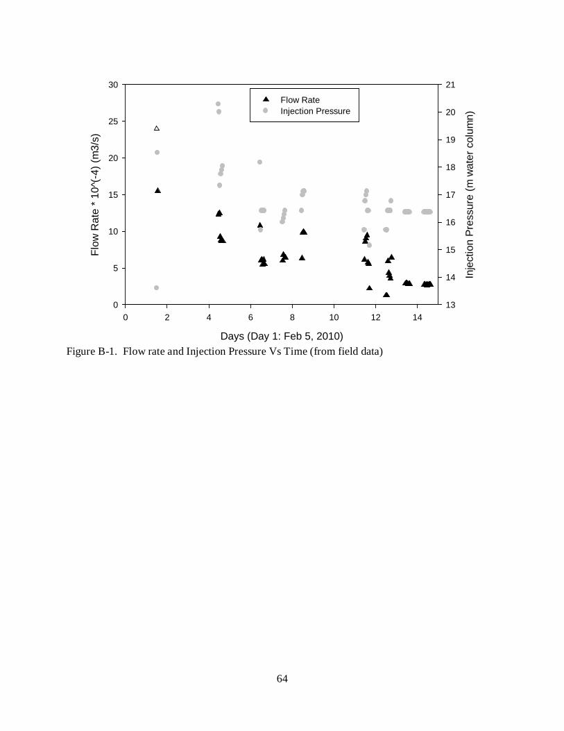
64

Days (Day 1: Feb 5, 2010)

0 2 4 6 8 10 12 14

Flow

Rat

e * 1

0^(-

4) (m

3/s)

0

5

10

15

20

25

30

Inje

ctio

n Pr

essu

re (m

wat

er c

olum

n)

13

14

15

16

17

18

19

20

21

Flow RateInjection Pressure

Figure B-1. Flow rate and Injection Pressure Vs Time (from field data)

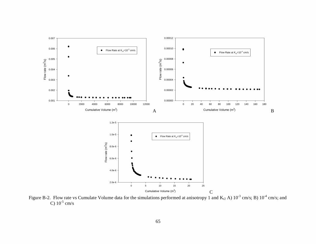
65

Cumulative Volume (m3)

0 2000 4000 6000 8000 10000 12000

Flow

rate

(m3 /s

)

0.001

0.002

0.003

0.004

0.005

0.006

0.007

Flow Rate at Kr2=10-3 cm/s

A Cumulative Volume (m3)

0 20 40 60 80 100 120 140 160 180

Flow

rate

(m3 /s

)

0.00000

0.00002

0.00004

0.00006

0.00008

0.00010

0.00012

Flow Rate at Kr2=10-4 cm/s

B

Cumulative Volume (m3)

0 5 10 15 20 25

Flow

rate

(m3 /s

)

2.0e-6

4.0e-6

6.0e-6

8.0e-6

1.0e-5

1.2e-5

Flow Rate at Kr2=10-5 cm/s

C Figure B-2. Flow rate vs Cumulate Volume data for the simulations performed at anisotropy 1 and Kr2 A) 10-3 cm/s; B) 10-4 cm/s; and

C) 10-5 cm/s

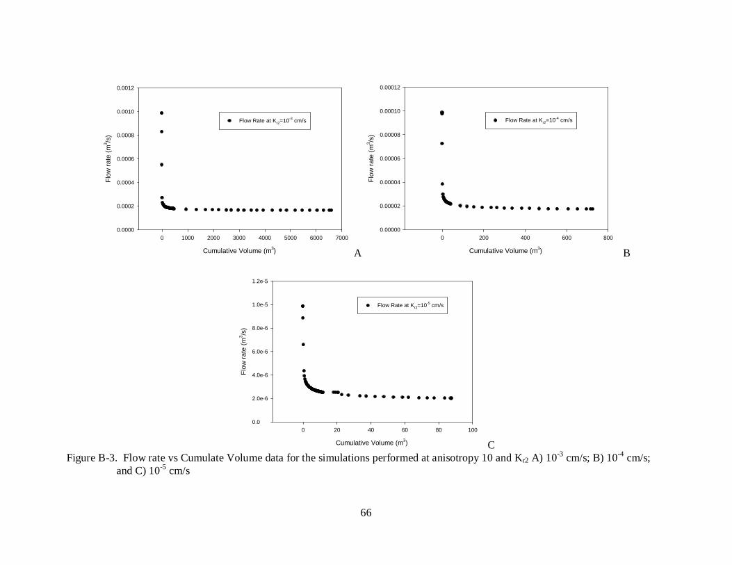
66

Cumulative Volume (m3)

0 1000 2000 3000 4000 5000 6000 7000

Flow

rate

(m3 /s

)

0.0000

0.0002

0.0004

0.0006

0.0008

0.0010

0.0012

Flow Rate at Kr2=10-3 cm/s

A Cumulative Volume (m3)

0 200 400 600 800

Flow

rate

(m3 /s

)

0.00000

0.00002

0.00004

0.00006

0.00008

0.00010

0.00012

Flow Rate at Kr2=10-4 cm/s

B

Cumulative Volume (m3)

0 20 40 60 80 100

Flow

rate

(m3 /s

)

0.0

2.0e-6

4.0e-6

6.0e-6

8.0e-6

1.0e-5

1.2e-5

Flow Rate at Kr2=10-5 cm/s

C Figure B-3. Flow rate vs Cumulate Volume data for the simulations performed at anisotropy 10 and Kr2 A) 10-3 cm/s; B) 10-4 cm/s;

and C) 10-5 cm/s

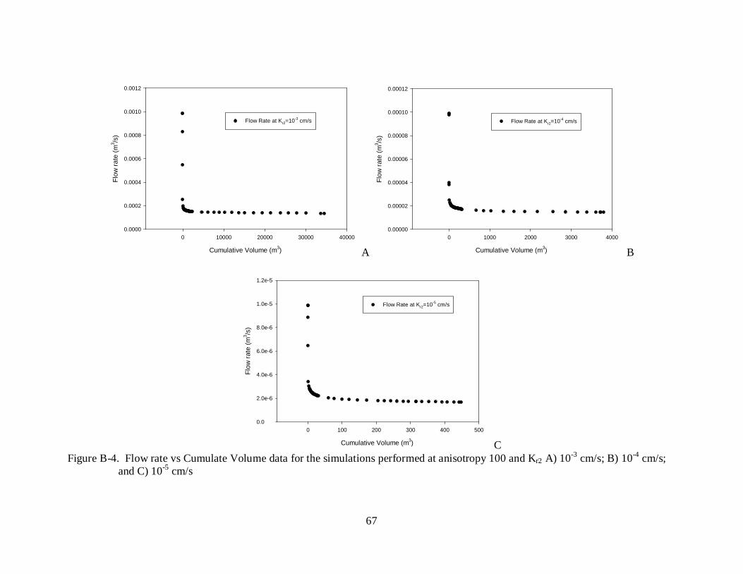
67

Cumulative Volume (m3)

0 10000 20000 30000 40000

Flow

rate

(m3 /s

)

0.0000

0.0002

0.0004

0.0006

0.0008

0.0010

0.0012

Flow Rate at Kr2=10-3 cm/s

A Cumulative Volume (m3)

0 1000 2000 3000 4000

Flow

rate

(m3 /s

)

0.00000

0.00002

0.00004

0.00006

0.00008

0.00010

0.00012

Flow Rate at Kr2=10-4 cm/s

B

Cumulative Volume (m3)

0 100 200 300 400 500

Flow

rate

(m3 /s

)

0.0

2.0e-6

4.0e-6

6.0e-6

8.0e-6

1.0e-5

1.2e-5

Flow Rate at Kr2=10-5 cm/s

C Figure B-4. Flow rate vs Cumulate Volume data for the simulations performed at anisotropy 100 and Kr2 A) 10-3 cm/s; B) 10-4 cm/s;

and C) 10-5 cm/s

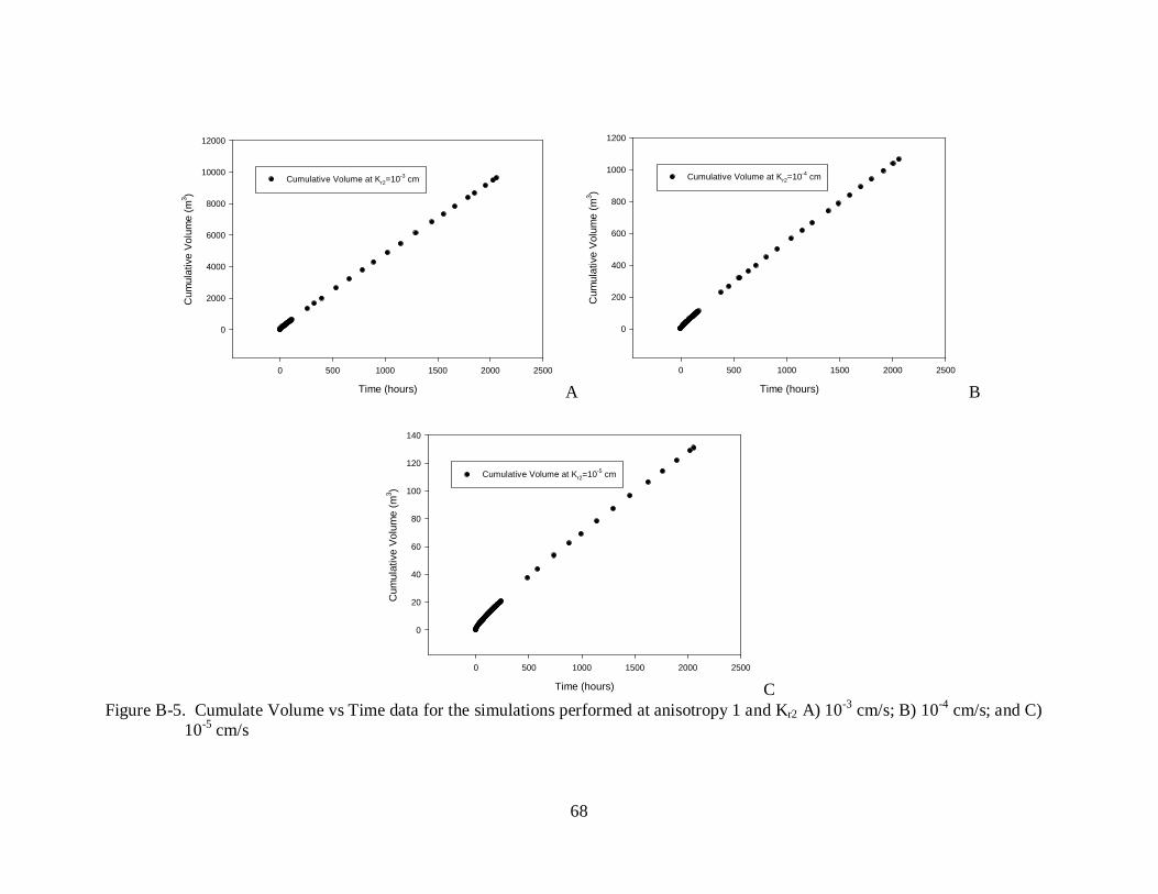
68

Time (hours)

0 500 1000 1500 2000 2500

Cum

ulat

ive

Volu

me

(m3 )

0

2000

4000

6000

8000

10000

12000

Cumulative Volume at Kr2=10-3 cm

A Time (hours)

0 500 1000 1500 2000 2500

Cum

ulat

ive

Volu

me

(m3 )

0

200

400

600

800

1000

1200

Cumulative Volume at Kr2=10-4 cm

B

Time (hours)

0 500 1000 1500 2000 2500

Cum

ulat

ive

Volu

me

(m3 )

0

20

40

60

80

100

120

140

Cumulative Volume at Kr2=10-5 cm

C Figure B-5. Cumulate Volume vs Time data for the simulations performed at anisotropy 1 and Kr2 A) 10-3 cm/s; B) 10-4 cm/s; and C)

10-5 cm/s

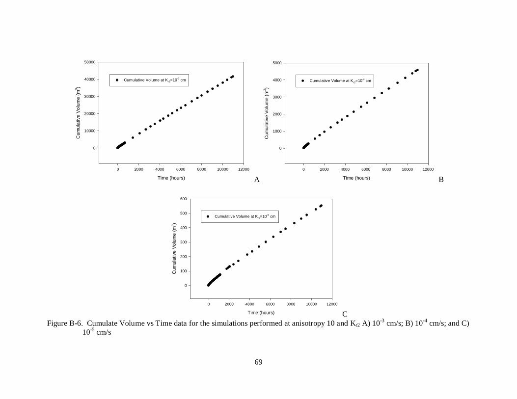
69

Time (hours)

0 2000 4000 6000 8000 10000 12000

Cum

ulat

ive

Volu

me

(m3 )

0

10000

20000

30000

40000

50000

Cumulative Volume at Kr2=10-3 cm

A Time (hours)

0 2000 4000 6000 8000 10000 12000

Cum

ulat

ive

Volu

me

(m3 )

0

1000

2000

3000

4000

5000

Cumulative Volume at Kr2=10-4 cm

B

Time (hours)

0 2000 4000 6000 8000 10000 12000

Cum

ulat

ive

Volu

me

(m3 )

0

100

200

300

400

500

600

Cumulative Volume at Kr2=10-5 cm

C Figure B-6. Cumulate Volume vs Time data for the simulations performed at anisotropy 10 and Kr2 A) 10-3 cm/s; B) 10-4 cm/s; and C)

10-5 cm/s

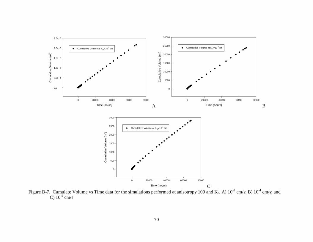
70

Time (hours)

0 20000 40000 60000 80000

Cum

ulat

ive

Volu

me

(m3 )

0.0

5.0e+4

1.0e+5

1.5e+5

2.0e+5

2.5e+5

Cumulative Volume at Kr2=10-3 cm

A Time (hours)

0 20000 40000 60000 80000

Cum

ulat

ive

Volu

me

(m3 )

0

5000

10000

15000

20000

25000

30000

Cumulative Volume at Kr2=10-4 cm

B

Time (hours)

0 20000 40000 60000 80000

Cum

ulat

ive

Volu

me

(m3 )

0

500

1000

1500

2000

2500

3000

Cumulative Volume at Kr2=10-5 cm

C Figure B-7. Cumulate Volume vs Time data for the simulations performed at anisotropy 100 and Kr2 A) 10-3 cm/s; B) 10-4 cm/s; and

C) 10-5 cm/s

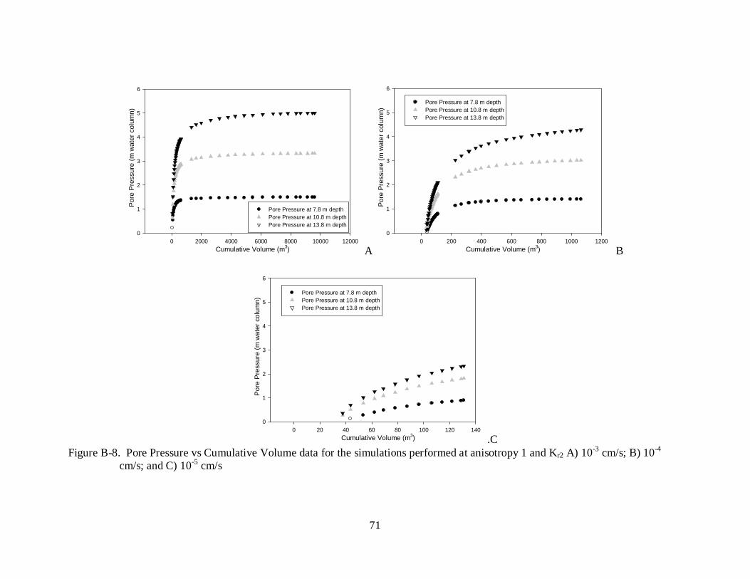
71

Cumulative Volume (m3) 0 2000 4000 6000 8000 10000 12000

Pore

Pre

ssur

e (m

wat

er c

olum

n)

0

1

2

3

4

5

6

Pore Pressure at 7.8 m depthPore Pressure at 10.8 m depthPore Pressure at 13.8 m depth

A Cumulative Volume (m3) 0 200 400 600 800 1000 1200

Pore

Pre

ssur

e (m

wat

er c

olum

n)

0

1

2

3

4

5

6

Pore Pressure at 7.8 m depthPore Pressure at 10.8 m depthPore Pressure at 13.8 m depth

B

Cumulative Volume (m3) 0 20 40 60 80 100 120 140

Pore

Pre

ssur

e (m

wat

er c

olum

n)

0

1

2

3

4

5

6

Pore Pressure at 7.8 m depthPore Pressure at 10.8 m depthPore Pressure at 13.8 m depth

.C Figure B-8. Pore Pressure vs Cumulative Volume data for the simulations performed at anisotropy 1 and Kr2 A) 10-3 cm/s; B) 10-4

cm/s; and C) 10-5 cm/s

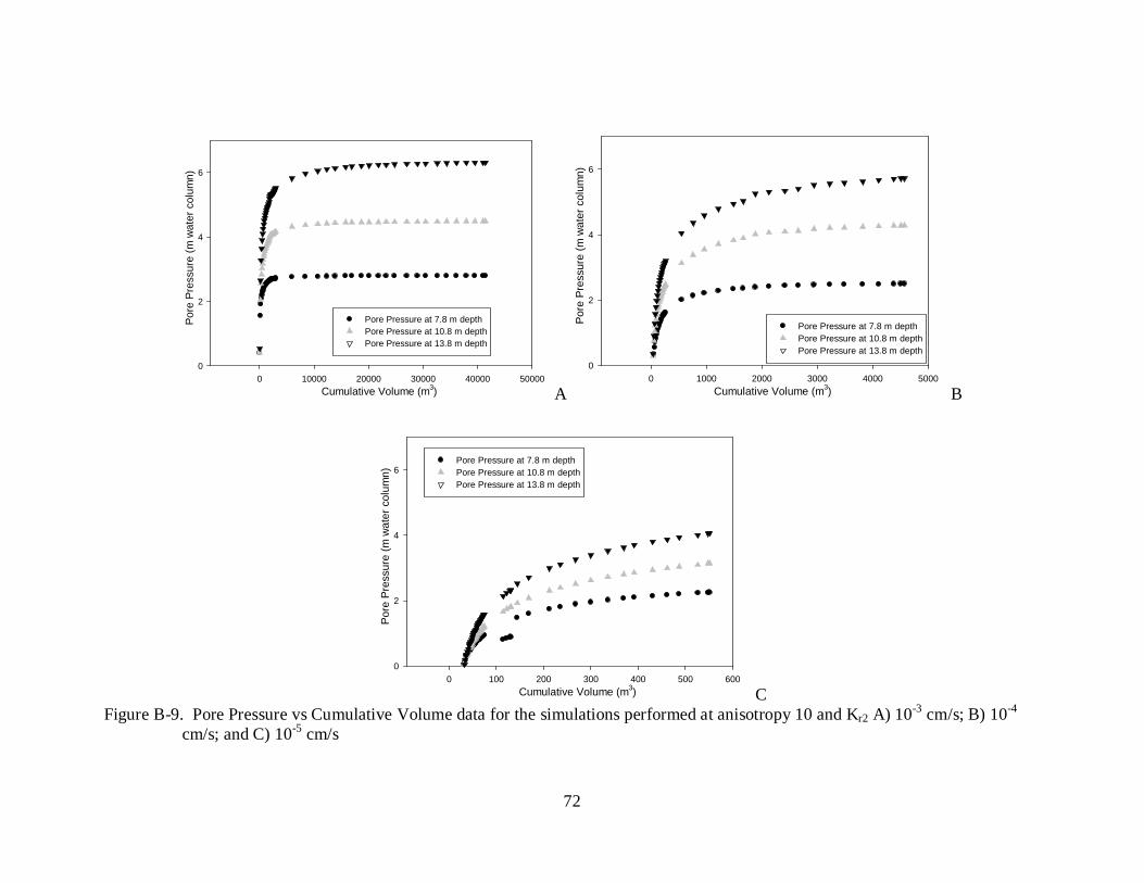
72

Cumulative Volume (m3) 0 10000 20000 30000 40000 50000

Pore

Pre

ssur

e (m

wat

er c

olum

n)

0

2

4

6

Pore Pressure at 7.8 m depthPore Pressure at 10.8 m depthPore Pressure at 13.8 m depth

A Cumulative Volume (m3) 0 1000 2000 3000 4000 5000

Pore

Pre

ssur

e (m

wat

er c

olum

n)

0

2

4

6

Pore Pressure at 7.8 m depthPore Pressure at 10.8 m depthPore Pressure at 13.8 m depth

B

Cumulative Volume (m3) 0 100 200 300 400 500 600

Pore

Pre

ssur

e (m

wat

er c

olum

n)

0

2

4

6Pore Pressure at 7.8 m depthPore Pressure at 10.8 m depthPore Pressure at 13.8 m depth

C Figure B-9. Pore Pressure vs Cumulative Volume data for the simulations performed at anisotropy 10 and Kr2 A) 10-3 cm/s; B) 10-4

cm/s; and C) 10-5 cm/s

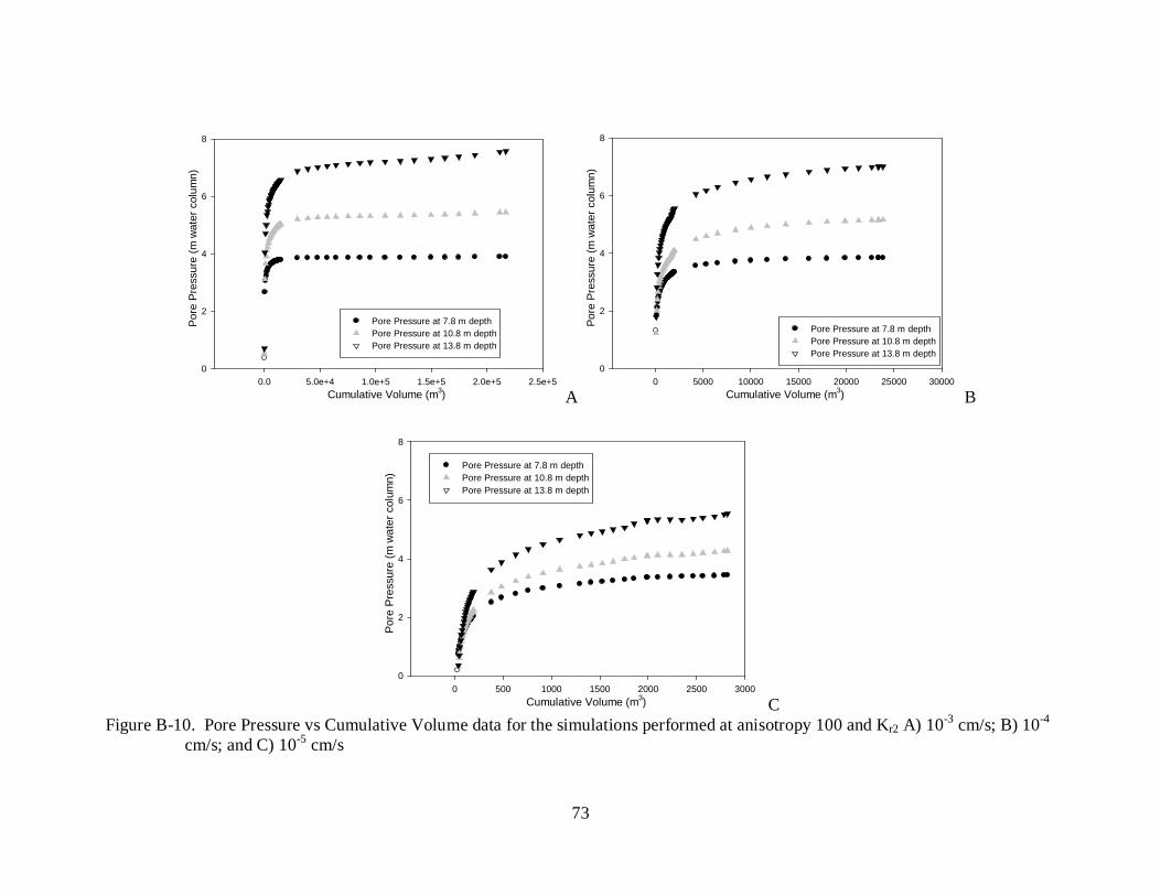
73

Cumulative Volume (m3) 0.0 5.0e+4 1.0e+5 1.5e+5 2.0e+5 2.5e+5

Pore

Pre

ssur

e (m

wat

er c

olum

n)

0

2

4

6

8

Pore Pressure at 7.8 m depthPore Pressure at 10.8 m depthPore Pressure at 13.8 m depth

A Cumulative Volume (m3) 0 5000 10000 15000 20000 25000 30000

Pore

Pre

ssur

e (m

wat

er c

olum

n)

0

2

4

6

8

Pore Pressure at 7.8 m depthPore Pressure at 10.8 m depthPore Pressure at 13.8 m depth

B

Cumulative Volume (m3) 0 500 1000 1500 2000 2500 3000

Pore

Pre

ssur

e (m

wat

er c

olum

n)

0

2

4

6

8

Pore Pressure at 7.8 m depthPore Pressure at 10.8 m depthPore Pressure at 13.8 m depth

C Figure B-10. Pore Pressure vs Cumulative Volume data for the simulations performed at anisotropy 100 and Kr2 A) 10-3 cm/s; B) 10-4

cm/s; and C) 10-5 cm/s

74

APPENDIX B CONSTRUCTION PHOTOGRAPHS FOR CHAPTER 3

This appendix presents the construction photographs for the installation of surface

infiltration trenches with whole tires as a bedding material.

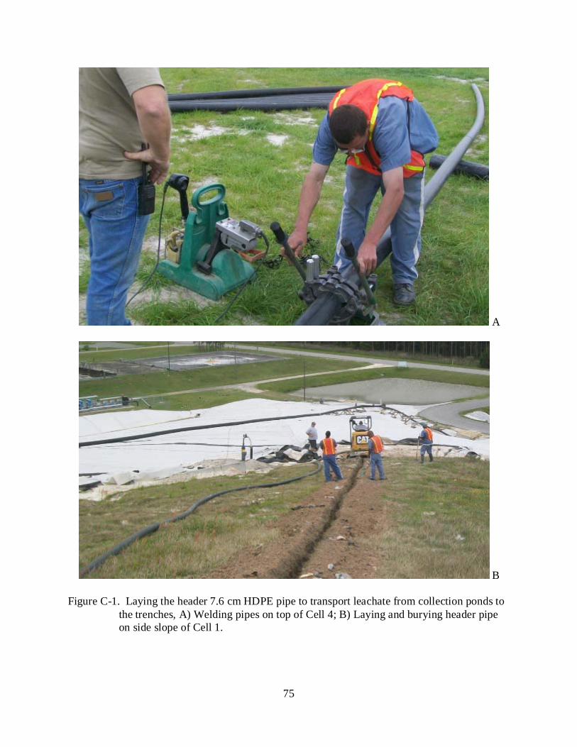
75

A

B

Figure C-1. Laying the header 7.6 cm HDPE pipe to transport leachate from collection ponds to the trenches, A) Welding pipes on top of Cell 4; B) Laying and burying header pipe on side slope of Cell 1.

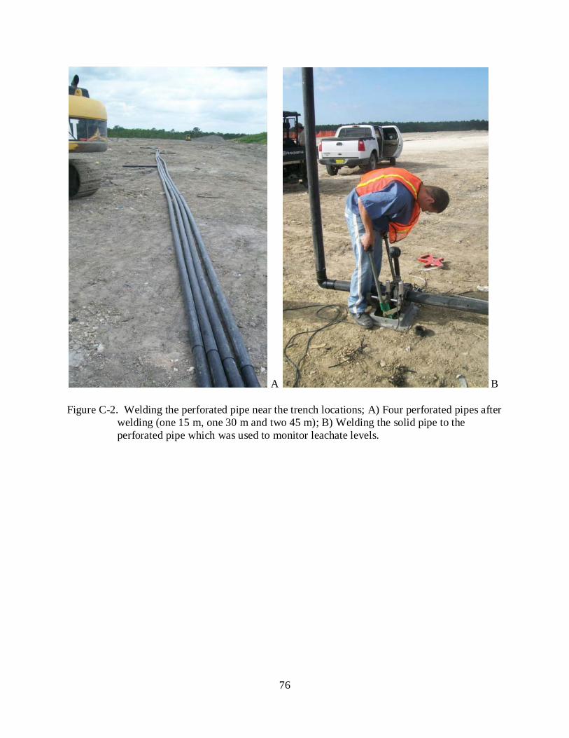
76

A B Figure C-2. Welding the perforated pipe near the trench locations; A) Four perforated pipes after

welding (one 15 m, one 30 m and two 45 m); B) Welding the solid pipe to the perforated pipe which was used to monitor leachate levels.

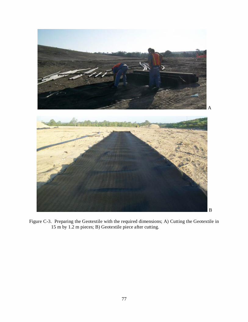
77

A

B Figure C-3. Preparing the Geotextile with the required dimensions; A) Cutting the Geotextile in

15 m by 1.2 m pieces; B) Geotextile piece after cutting.

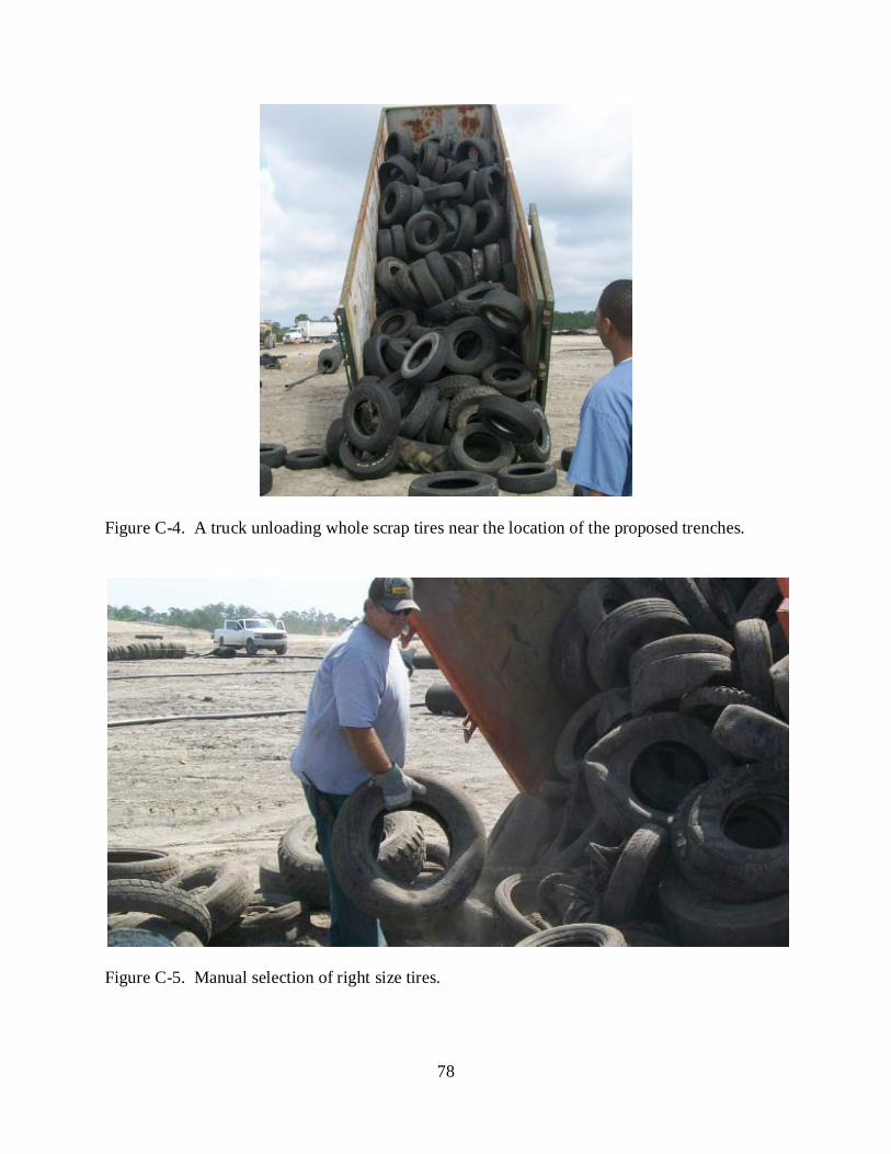
78

Figure C-4. A truck unloading whole scrap tires near the location of the proposed trenches.

Figure C-5. Manual selection of right size tires.

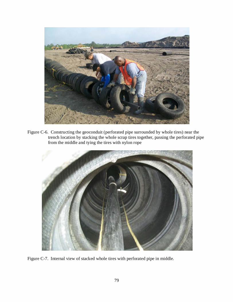
79

Figure C-6. Constructing the geoconduit (perforated pipe surrounded by whole tires) near the trench location by stacking the whole scrap tires together, passing the perforated pipe from the middle and tying the tires with nylon rope

Figure C-7. Internal view of stacked whole tires with perforated pipe in middle.

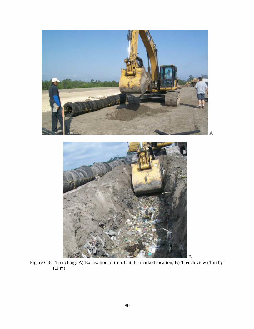
80

A

B Figure C-8. Trenching: A) Excavation of trench at the marked location; B) Trench view (1 m by

1.2 m)

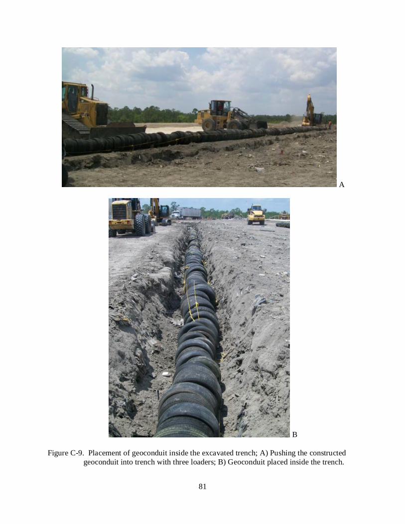
81

A

B

Figure C-9. Placement of geoconduit inside the excavated trench; A) Pushing the constructed geoconduit into trench with three loaders; B) Geoconduit placed inside the trench.

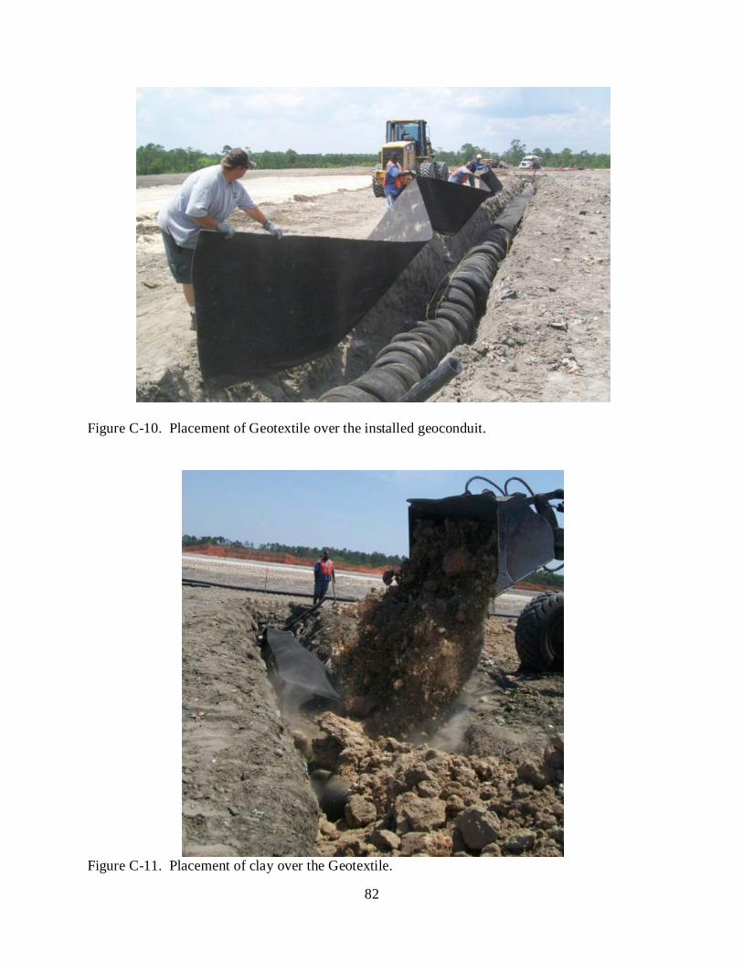
82

Figure C-10. Placement of Geotextile over the installed geoconduit.

Figure C-11. Placement of clay over the Geotextile.

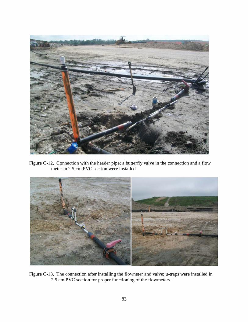
83

Figure C-12. Connection with the header pipe; a butterfly valve in the connection and a flow

meter in 2.5 cm PVC section were installed.

Figure C-13. The connection after installing the flowneter and valve; u-traps were installed in

2.5 cm PVC section for proper functioning of the flowmeters.

84

LIST OF REFERENCES Al-Yousfi, A.B. and and Pohland, F.G. (1998). “Strategies for simulation, design, and

management of solid wastes disposal sites as landfill bioreactors.” Practice Periodical of Hazardous, Toxic, and Radioactive Waste Management, 13-21.

Ardejani, F.D., Badii, Kh., Limaee, N.Y., Mahmoodi, N.M., Arami, M., Shafaei, S.Z., Mirhabibi, A.R., (2006). “Numerical modelling and laboratory studies on the removal of Direct Red 23 and Direct Red 80 dyes from textile effluents using orange peel, a low-cost adsorbent.” Dyes and Pigments 73 (2007) 178e185.

Benson, C. H., Barlaz, M. A., Lane, D. T., and Rawe, J. M., B.E. (2007). “Practice review of five bioreactor/recirculation landfills.” Waste Management, 27,13-29.

Bleiker, E.D., McBean, E., and Farquhar, G. (1993). “Refuse Sampling and Permeability Testing at the Brock Westand Keele Valley Landfills.” Proceedings, Sixteenth International Madison Waste Conference: municipal & industrial waste, September 22-23, 1993. 548-567.

Durmusoglu, E., Sanchez, M. Itza and Corapcioglu, Y. M. (2006). “Permeability and compression characteristics of Municipal solid waste.” Environ Geol., 50, 773-789.

Gabr, M. A., and Valero, S. N. (1995). “Geotechnical Properties of Municipal Solid Waste.” Geotechnical Testing Journal, 18(2), 241-255.

Haydar, M and Khire, M. (2004). “Evaluation of heterogeneity and anisotropy of waste properties on leachate recirculation in bioreactor landfills.” Journal of Solid Waste Technology and Management, 30(4), 233–242.

Haydar, M., and Khire, M. (2005). “Leachate recirculation using horizontal trenches in bioreactor landfills.” Journal of Geotechnical and Geoenvironmental Engineering, ASCE, 131(7), 837–847.

Hudson, A. P., Beaven, R. P., and Powrie, W. (1999). “Measurement of the horizontal hydraulic conductivity of household waste in a large scale compression cell.” Proceedings Sardinia 99, Seventh International Waste Management and Landfill Symposium, S. Margherita di Pula, Cagliari, Italy; 4-8 October 1999.

Hudson A. P., White J. K., Beaven R. P., Powrie W. (2004). “Modelling the compression behaviour of landfilled domestic waste.” Waste Management 24, 259-269.

Jain, P. (2005). “Moisture addition at bioreactor landfills using vertical wells: Mathematical modeling and field application.” Ph.D. Dissertation. University of Florida, Gainesville, FL, U.S.A.

85

Jain, P., Farfour, W. M., Jonnalagadda, S., Townsend, T. G., and Reinhart, D. R. (2005a). “Performance evaluation of vertical wells for landfill leachate recirculation.” Proceedings of Geo Frontier 2005, ASCE conference, January 24-26, Austin, TX, U.S.A.

Jain, P., Powell, J. P., Townsend, T. G., and Reinhart, D. R. (2005b). “Air permeability of waste in a municipal solid waste landfill.” Journal of Environmental Engineering, ASCE, 131(11) 1565-1573.

Jain, P., Powell, J., Townsend, T. G., and Reinhart, D, R. (2006). “Estimating The Hydraulic Conductivity of Landfilled Municipal Solid Waste Using Borehole Permeameter Test.” Journal of Environmental engineering, ASCE, 132(6), 645-653.

Jain, P., Townsend, T. G., and Tolaymat, T. M. (2010). “Steady-state design of vertical wells for liquids addition at bioreactor landfills.” Waste Management, Elsevier, in press.

Jang, Y.S., Kim Y.W., and Lee S.I. (2002). “Hydraulic properties and leachate level analysis of Kimpo metropolitan Landfill, Korea.” Waste Management, 22, 261-267.

Kadambala, R. (2009). “Evaluation of a buried vertical well leachate recirculation system and settlement resulting from moisture addition using vertical wells for municipal solid waste landfills.” Ph.D. Dissertation. University of Florida, Gainesville, FL, U.S.A.

Khire, M. and Mukherjee, M. (2006). “Leachate Injection Using Vertical Wells in Engineered Landfills.” Waste Management, Elsevier, in press.

Koerner, R. G., and Eith, W. A. (2005). “Drainage capability of fully degraded MSW with respect to various leachate collection and removal systems.” Geotechnical special publication 130, 4233-4237.

Landva, A. O., Pelkey, S. G., and Valsangkar, A. J. (1998). “Coefficient of permeability of municipal refuse.” Proceedings of the Third International Congress on Environmental Geotechnics, Balkema, Rotterdam, 163-67.

Larson, J. A. (2007). “Investigations at a Bioreactor Landfill to Aid in the Operation and Design of Horizontal Injection Liquids Addition Systems.” Master’s Thesis, University of Florida, Gainesville, FL, U.S.A.

Maier, T.B. (1998). “Analysis procedures for design of leachate recirculation systems.” Water Quality International, Nov-Dec 1998, 37-40.

McCreanor, P.T. and Reinhart, D.R (1996). “Hydrodynamic modeling of leachate recirculating landfills.” Wat. Sci. Tech., 34(7-8), 463-70.

McCreanor, P.T. (1998). “Landfill Leachate Recirculation Systems: Mathematical Modeling and Validation.” Ph.D. Dissertation. University of Central Florida.

McCreanor, P.T. and Reinhart, D.R. (2000). “Mathematical Modeling of Leachate Routing in a Leachate Recirculating Landfill.” Water Research, 34(4), 1285-1295.

86

Mehta, R., Barlaz, M.A., Yazdani, R., Augenstein, D., Bryars, M., and Sinderson, L. (2002).

“Refuse Decomposition in the Presence and Absence of Leachate Recirculation.” Journal of Environmental Engineering, March 2002, 228-236.

Pacey, J. P., Ramin Yazdani, D. Reinhart, R. Morck, D. Augenstein (1999). “The Bioreactor Landfill: An Innovation in Solid Waste Management.” SWANA, Silver Springs, Maryland.

Pohland, F.G. (1975). Sanitary landfill stablization with leachate recycle and residual treatment. EPA-600/2-75-043. U.S. EPA, Washington DC, U.S.A.

Pohland, Fredrick (1980). “Leachate recycle as landfill management option.” Journal of Environmental Engineering, ASCE, 106 (EE6), 1057–1069.

Pohland, F.G. and Harper, S.R. (1986). Critical review and summary of leachate and gas production from landfills. EPA/600/2-86/073. Cincinnati, OH, U.S.A.: U.S. Environmental Protection agency.

Powrie, W and Beaven R.P. (1999). “Hydraulic Properties of Household Waste and Applications for Landfills.” Proceedings Institution of civil Engineers, Geotechnical Engineering, 137, 235-247.

Powrie, W., Beaven, R., Hudson, A., 2008. “The influence of landfill gas on the hydraulic conductivity of waste.” Geotechnical Special Publication No. 177, Geocongress 2008, Geotechnics of Waste Management and Remediaton, March 9, 2008, New Orleans, Louisiana, pp. 264–271.

Reinhart D.R. and Townsend T.G. (1997). Landfill Bioreactor Design and Operation. Lewis Publishers, Boca Raton FL.

Reinhart, D.R., McCreanor, P.T., and Townsend, T.G. (2002). “The bioreactor landfill: Its status and future.” Waste Management and Research. 20: 172-186.

Shank, K.L. (1993). “Determination of hydraulic conductivity of the Alachua County Southwest Landfill.” Master's thesis, University of Florida.

Tchobanoglous, G., Theisen, H., and Vigil, S. (1993). Integrated solid waste management. McGraw-Hill, New York, U.S.A.

Townsend, T. G., (1995). “Leachate recycle at solid waste landfills using horizontal injection.” Ph.D. Dissertation, University of Florida, Gainesville, FL, U.S.A.

Townsend, T. G., Miller W. L., and Earle, J. F. K (1995). “Leachate recycle infiltration ponds.” Journal of Environmental Engineering, ASCE, 121(6), 465–471.

Townsend, T. G., Miller, W. L, Lee, H. J., and Earle, J. F. K (1996). “Acceleration of landfill stabilization using leachate recycle.” Journal of Environmental Engineering, ASCE, 122(4), 263-268.

87

Townsend, T. G. and Miller W. L. (1998). “Leachate recycle using horizontal injection.” Advances of Environmental Research, 2(2) 1995, 129–138.

U.S. EPA (2006). Scrap tire cleanup guidebook. January 2006. U.S. EPA (2007). Bioreactor Landfills. June 2007. U.S. EPA (2008). Municipal Solid Waste in the United States: 2007 Facts and Figures. Office of

Solid Waste and Emergency Response EPA530-R-08-010, November 2008.

Woyshner, M.R. and Yanful, E.K. (1995). “Modelling and field measurements of water percolation through an experimental soil cover on mine tailings.” Canadian Geotechnical Journal 32(4): 601–609 (1995).

88

BIOGRAPHICAL SKETCH

Karamjit Singh was born in Punjab, India, to Harmeet Singh and Tejinder Kaur. He

graduated with a Bachelor of Engineering in civil engineering from Punjab Engineering College,

Chandigarh, India in July, 2008. In August 2008, he enrolled in graduate school in the

Environmental Engineering Sciences Department at the University of Florida, to study solid and

hazardous waste management under the advisement of Dr. Timothy Townsend.