© 2009 McGraw-Hill Ryerson Limited 7-1 Chapter 7 Common Stock Valuation CHAPTER OUTLINE Security analysis Security analysis The dividend discount model

© 2009 McGraw-Hill Ryerson Limited 7-1

Chapter 7Common Stock

Valuation

CHAPTER OUTLINE•Security analysis•The dividend discount model•The two-stage dividend growth

model•The residual Income Model•Price ratio analysis•An analysis of McGraw-Hill

Company


Security Analysis Fundamental analysis is a term for studying a

company’s accounting statements and other financial and economic information to estimate the economic value of a company’s stock.

The basic idea is to identify “undervalued” stocks to buy and “overvalued” stocks to sell.In practice however, such stocks may in fact be correctly priced for reasons not immediately apparent to the analyst.


The Dividend Discount Model

The Dividend Discount Model (DDM) is a method to estimate the value of a share of stock by discounting all expected future dividend payments. The DDM equation is:

In the DDM equation: V(0) = the present value of all future dividends D(t) = the dividend to be paid t years from now k = the appropriate risk-adjusted discount rate

T32 k1

D(T)

k1

D(3)

k1

D(2)

k1

D(1)V(0)


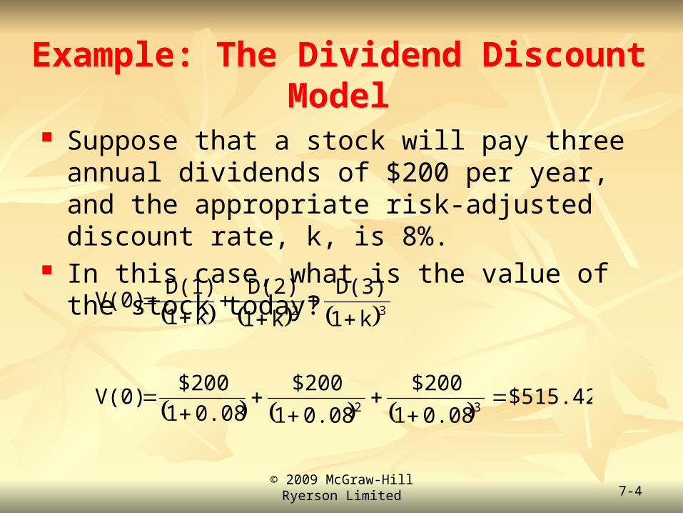
Example: The Dividend Discount Model

Suppose that a stock will pay three annual dividends of $200 per year, and the appropriate risk-adjusted discount rate, k, is 8%.

In this case, what is the value of the stock today?

$515.42

0.081

$200

0.081

$200

0.081

$200V(0)

k1

D(3)

k1

D(2)

k1

D(1)V(0)

32

32


The Dividend Discount Model: the Constant Growth Rate Model

Assume that the dividends will grow at a constant growth rate g.

Then, the dividend next period (t + 1) is:

In this case, the DDM formula becomes:

g k if D(0) T V(0)

g k if k1

g11

gk

g)D(0)(1V(0)

T

g1tD1tD


Example: The Constant Growth Rate Model

Suppose the current dividend is $10, the dividend growth rate is 10%, there will be 20 yearly dividends, and the appropriate discount rate is 8%. What is the value of the stock, based on the constant growth rate model?

$243.86

1.08

1.101

.10.08

1.10$100V

g k if k1

g11

gk

g)D(0)(1V(0)

20

T


The Constant Perpetual Growth Model.

Assuming that the dividends will grow forever at a constant growth rate g.

In this case, the DDM formula becomes:

kg

gk

1D

gk

g10D0V


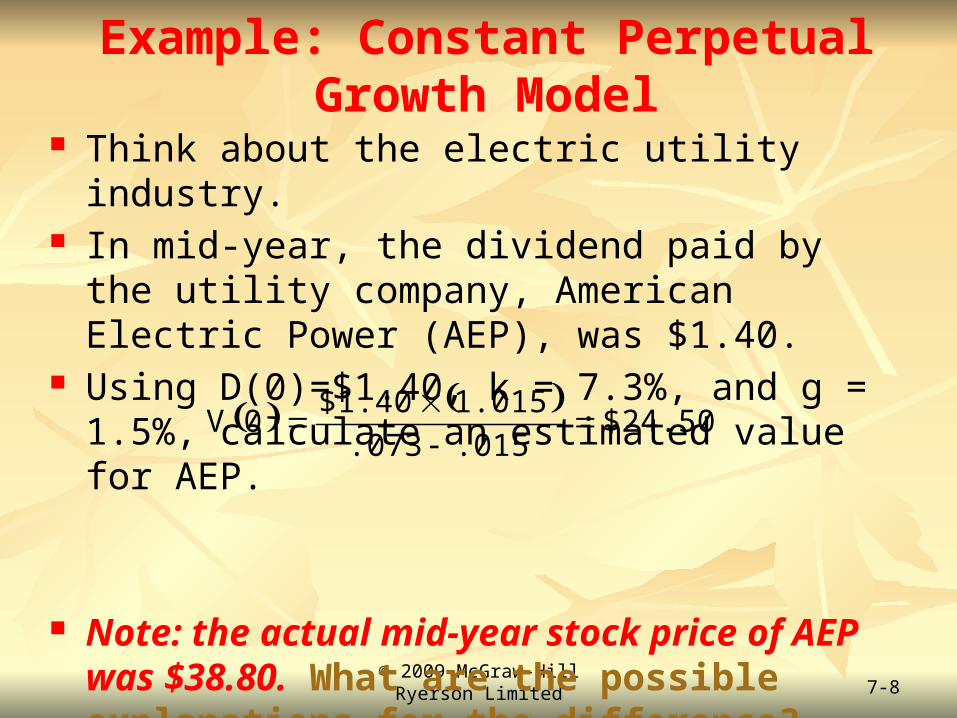
Example: Constant Perpetual Growth Model

Think about the electric utility industry. In mid-year, the dividend paid by the utility company,

American Electric Power (AEP), was $1.40. Using D(0)=$1.40, k = 7.3%, and g = 1.5%, calculate

an estimated value for AEP.

Note: the actual mid-year stock price of AEP was $38.80. What are the possible explanations for the difference?

$24.50

.015.073

1.015$1.400V


Estimating the Growth Rate

The growth rate in dividends (g) can be estimated in a number of ways. Using the company’s historical average growth rate. Using an industry median or average growth rate. Using the sustainable growth rate.

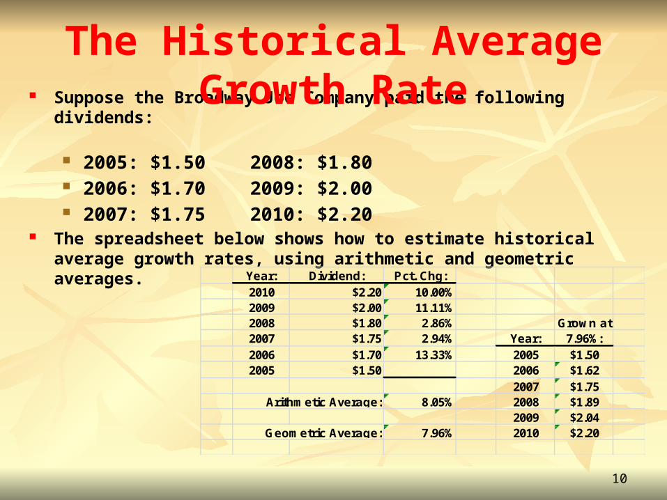
Suppose the Broadway Joe Company paid the following dividends:

2005: $1.50 2008: $1.80 2006: $1.70 2009: $2.00 2007: $1.75 2010: $2.20

The spreadsheet below shows how to estimate historical average growth rates, using arithmetic and geometric averages.

Year: Dividend: Pct. Chg:2010 $2.20 10.00%2009 $2.00 11.11%2008 $1.80 2.86% Grown at2007 $1.75 2.94% Year: 7.96%:2006 $1.70 13.33% 2005 $1.502005 $1.50 2006 $1.62

2007 $1.758.05% 2008 $1.89

2009 $2.047.96% 2010 $2.20

Arithmetic Average:

Geometric Average:

10

The Historical Average Growth Rate


The Sustainable Growth Rate

Return on Equity (ROE) = Net Income / Equity

Payout Ratio = Proportion of earnings paid out as dividends

Retention Ratio = Proportion of earnings retained for investment

Ratio)Payout - (1 ROE

RatioRetention ROE RateGrowth eSustainabl


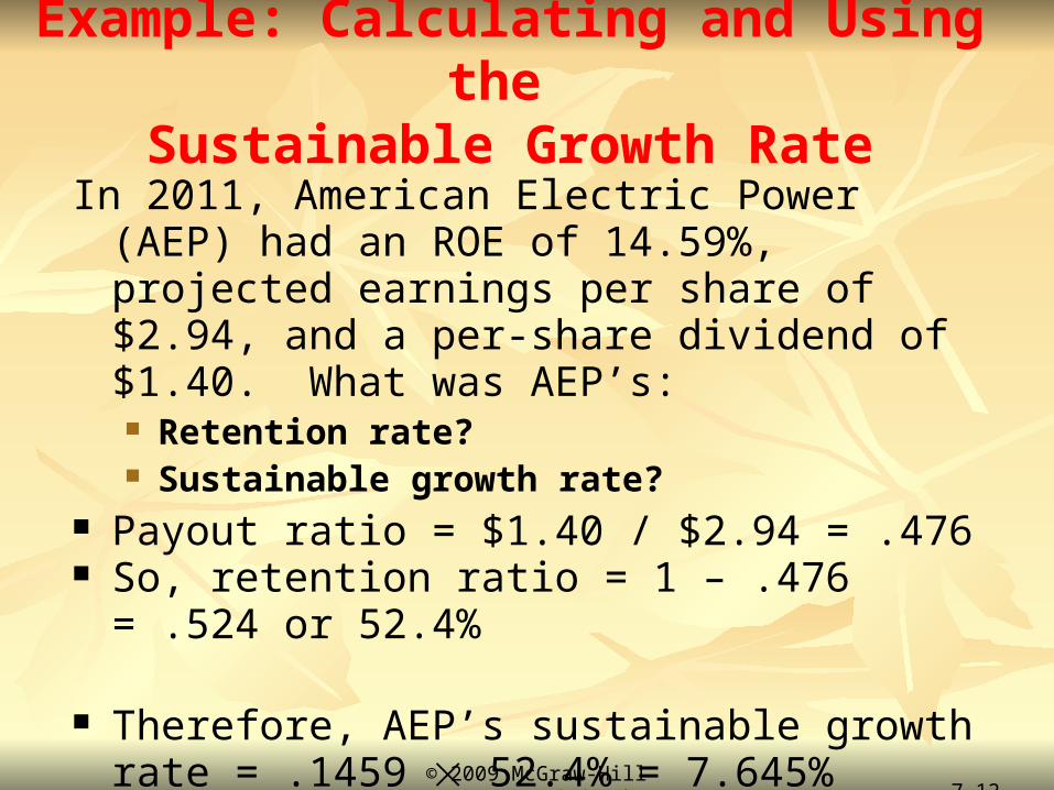
Example: Calculating and Using the Sustainable Growth Rate

In 2011, American Electric Power (AEP) had an ROE of 14.59%, projected earnings per share of $2.94, and a per-share dividend of $1.40. What was AEP’s: Retention rate? Sustainable growth rate?

Payout ratio = $1.40 / $2.94 = .476 So, retention ratio = 1 – .476 = .524 or 52.4%

Therefore, AEP’s sustainable growth rate = .1459 52.4% = 7.645%


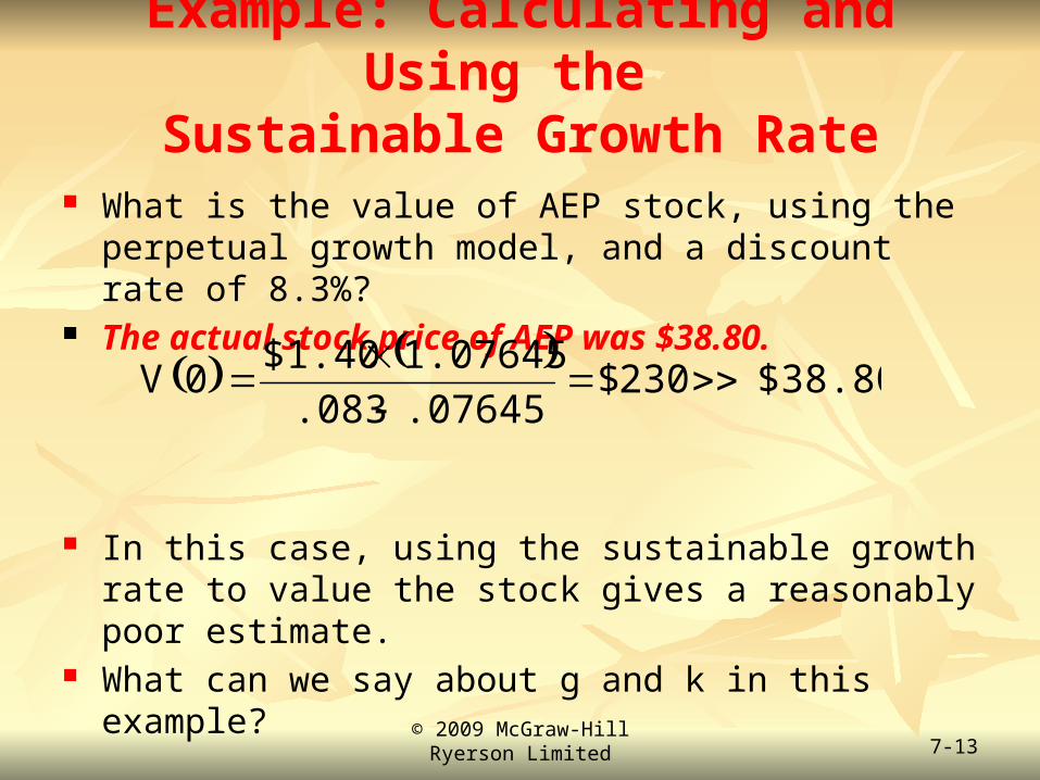
Example: Calculating and Using the Sustainable Growth Rate

What is the value of AEP stock, using the perpetual growth model, and a discount rate of 8.3%?

The actual stock price of AEP was $38.80.

In this case, using the sustainable growth rate to value the stock gives a reasonably poor estimate.

What can we say about g and k in this example?

$38.80 230$

.07645.083

1.07645$1.400V

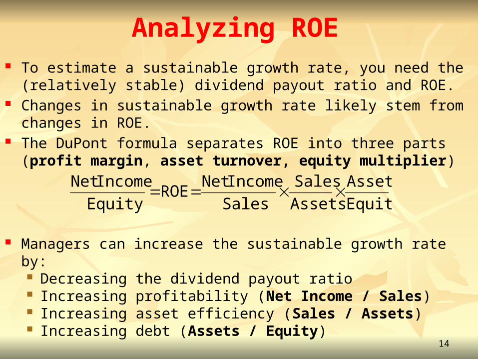
To estimate a sustainable growth rate, you need the (relatively stable) dividend payout ratio and ROE.

Changes in sustainable growth rate likely stem from changes in ROE. The DuPont formula separates ROE into three parts (profit margin,

asset turnover, equity multiplier)

Managers can increase the sustainable growth rate by: Decreasing the dividend payout ratio Increasing profitability (Net Income / Sales) Increasing asset efficiency (Sales / Assets) Increasing debt (Assets / Equity)

EquityAssets

AssetsSales

SalesIncome Net

ROEEquity

Income Net

14

Analyzing ROE


The Two-Stage Dividend Growth Model

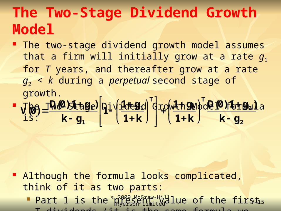
The two-stage dividend growth model assumes that a firm will initially grow at a rate g1 for T years, and thereafter grow at a rate g2 < k during a perpetual second stage of growth.

The Two-Stage Dividend Growth Model formula is:

Although the formula looks complicated, think of it as two parts: Part 1 is the present value of the first T dividends (it is the

same formula we used for the constant growth model). Part 2 is the present value of all subsequent dividends.

2

2

T

1

T

1

1

1

gk

)g1)(0(D

k1

g1

k1

g11

gk

)g1)(0(D)0(V

7-16

Two-Stage Dividend Growth Model

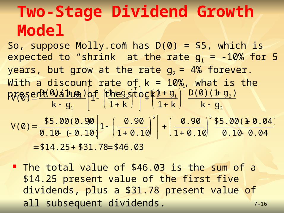
The total value of $46.03 is the sum of a $14.25 present value of the first five dividends, plus a $31.78 present value of all subsequent dividends.

$46.03 $31.78 $14.25

0.040.10

0.04)$5.00(1

0.101

0.90

0.101

0.901

0.10)(0.10

)$5.00(0.90V(0)

gk

)gD(0)(1

k1

g1

k1

g11

gk

)gD(0)(1V(0)

55

2

2

T

1

T

1

1

1

So, suppose Molly.com has D(0) = $5, which is expected to “shrink” at the rate g1 = -10% for 5 years, but grow at the rate g2 = 4% forever. With a discount rate of k = 10%, what is the present value of the stock?

7-17

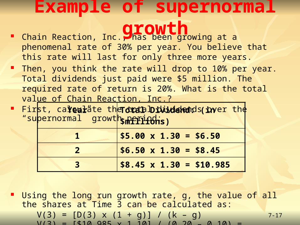
Example of supernormal growth Chain Reaction, Inc., has been growing at a phenomenal rate of 30% per year.

You believe that this rate will last for only three more years. Then, you think the rate will drop to 10% per year. Total dividends just paid

were $5 million. The required rate of return is 20%. What is the total value of Chain Reaction, Inc.?

First, calculate the total dividends over the “supernormal” growth period:

Using the long run growth rate, g, the value of all the shares at Time 3 can be calculated as:

V(3) = [D(3) x (1 + g)] / (k – g)V(3) = [$10.985 x 1.10] / (0.20 – 0.10) = $120.835

Year Total Dividend: (in $millions)

1 $5.00 x 1.30 = $6.50

2 $6.50 x 1.30 = $8.45

3 $8.45 x 1.30 = $10.985

7-18

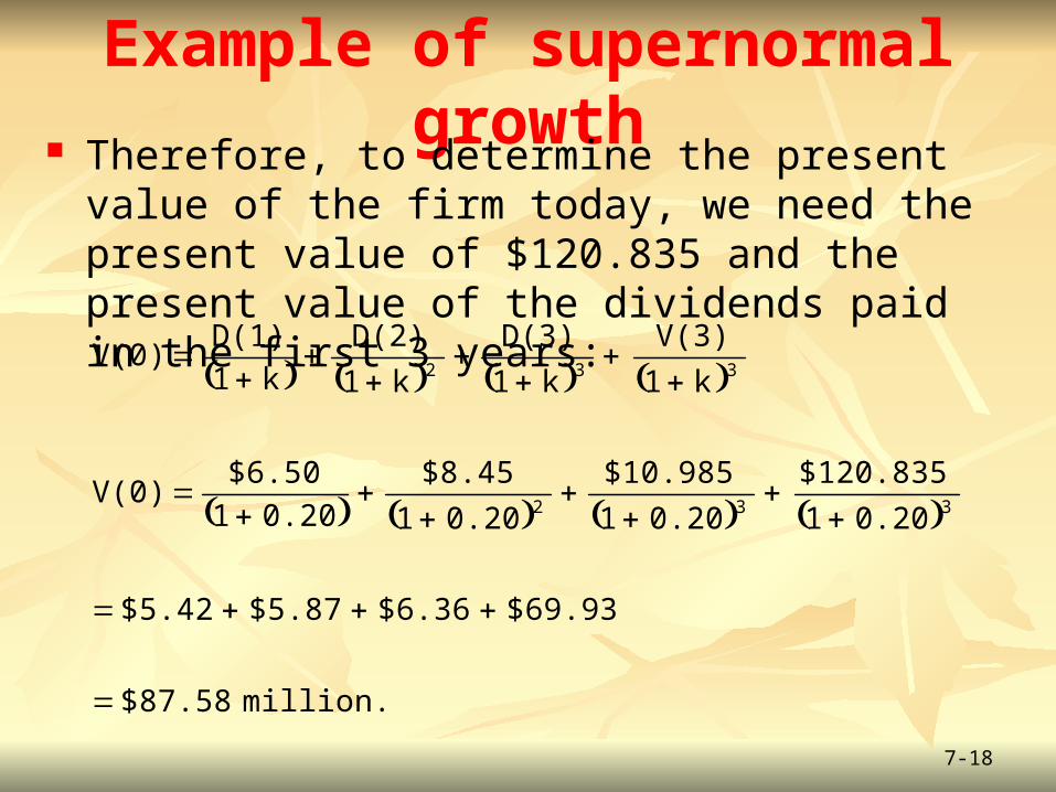
Example of supernormal growth Therefore, to determine the present value of the firm

today, we need the present value of $120.835 and the present value of the dividends paid in the first 3 years:

million. $87.58

$69.93$6.36$5.87$5.42

0.201

$120.835

0.201

$10.985

0.201

$8.45

0.201

$6.50V(0)

k1

V(3)

k1

D(3)

k1

D(2)

k1

D(1)V(0)

332

332


Discount Rates The discount rate for a stock can be estimated using the capital

asset pricing model (CAPM ). We will discuss the CAPM in a later chapter. However, we can estimate the discount rate for a stock using the

following formula: Discount rate = time value of money + risk premium

= T-bill rate + (stock beta x stock market risk premium)

T-bill rate: return on 90-day T-bills

Stock Beta: Risk relative to an average stock

Stock Market Risk Premium: Risk premium for an average stock


Observations on Dividend Discount Models

Constant Perpetual Growth Model:• Simple to compute• Not usable for firms that do not pay dividends• Not usable when g > k• Is sensitive to the choice of g and k• k and g may be difficult to estimate accurately.• Constant perpetual growth is often an unrealistic

assumption.


Two-Stage Dividend Growth Model:• More realistic in that it accounts for two stages of growth• Usable when g > k in the first stage• Not usable for firms that do not pay dividends• Is sensitive to the choice of g and k• k and g may be difficult to estimate accurately.

Observations on Dividend Discount Models


Residual Income Model (RIM) We have valued only companies that pay dividends.

But, there are many companies that do not pay dividends. What about them? It turns out that there is an elegant way to value these

companies, too. The model is called the Residual Income Model (RIM).Major Assumption (known as the Clean Surplus

Relationship, or CSR): The change in book value per share is equal to earnings per share minus dividends.


Residual Income Model (RIM) Inputs needed:

Earnings per share at time 0, EPS0

Book value per share at time 0, B0

Earnings growth rate, g Discount rate, k

There are two equivalent formulas for the Residual Income Model:

gk

gBEPSP

or

gk

kBg)(1EPSBP

010

0000

BTW, it turns out that the RIM is mathematically the same as the constant perpetual growth model.


Using the Residual Income Model. National Beverage Corporation (FIZ) It is July 1, 2005—shares are selling in the market

for $7.98. Using the RIM:

EPS0=$0.47 DIV = 0 B0=$4.271 g = 0.09 K = .103

What can we sayabout the marketprice of FIZ?

$9.84.$5.57$4.271P

.09.103

.103$4.271.09)(1$.47$4.271P

gk

kBg)(1EPSBP

0

0

0000

7-25

The Growth of FIZ

Using the information from the previous slide, what growth rate results in a FIZ price of $7.98?

8.42%.or .0842g

4.179g.3519

.0301.47g3.709g$.3820

.4399.47g.47g)(.103$3.709

g.103

.103$4.271g)(1$.47$4.271$7.98

gk

kBg)(1EPSBP 00

00

We can value companies that do not pay dividends using the residual income model.

Note: We assume positive earnings when we use the residual income model.

But, there are companies that do not pay dividends and have negative earnings.

Negative earnings = little value? We calculate earnings based on accounting rules and tax codes. It is possible that a company has:

negative earnings positive cash flows a positive value.

26

Free Cash Flow

Depreciation—the key to understand how a company can have negative earnings and positive cash flows

Depreciation reduces earnings because it is counted as an expense (more expenses = lower taxes paid).

Most stock analysts, however, use a relatively simple formula to calculate Free Cash Flow, FCF:

FCF = Net Income + Depreciation – Capital Spending

We can see that it is possible for: Net Income < 0 and FCF > 0

Depreciation and Capital Spending matter in FCF.

27

Free Cash Flow

The DDMs calculate a value of the equity only. DDMs use dividends, a cash flow only to equity holders DDMs use the CAPM to estimate required return DDMs use an equity beta to account for risk

Using the FCF model, we calculate a value for the firm. Free cash flow can be paid to debt holders and to stockholders. We can still calculate the value of equity using FCF

Calculate the value of the entire firm Subtract out the value of debt

We need a beta for assets, not the equity, to account for risk

28

DDM vs. FCF

Asset betas measure the risk of the company’s industry. Firms in an industry should have about the same asset betas. Their equity betas, however, could be quite different.

Investors can increase portfolio risk by using margin (i.e., borrowing money to buy stock).

A business can increase risk by using debt. So, to value the company, we must “convert” reported equity betas into

asset betas by adjusting for leverage. The following conversion formula is widely used:

What happens when a firm has no debt?

)](1EquityDebt

[1AssetEquity tBB

tax rate.

29

Asset Betas

Inputs An estimate of FCF:

Net Income Depreciation Capital Expenditures

The growth rate of FCF The proper discount rate Tax rate Debt/Equity ratio Equity beta

Calculate value using a “DDM” formula

“DDM” because we are using FCF, not dividends.30

The FCF Approach, Example

An estimate of FCF: Net Income: $25 million Depreciation: $10 million Capital Expenditures: $3 million Growth rate of FCF: 3% Tax rate: 35% Debt/Equity ratio: .40 Equity beta: 1.2

Asset Beta: 1.2 = BAsset x [1+.4 x (1-.35)]

1.2 = BAsset x 1.26

BAsset = 0.95

The proper discount rate: k = 4.00 + (7.00 × 0.95) = 10.65%

Assume: No dividends Risk-free rate = 4% Market risk premium = 7%

shares. ofnumber million / $330.85 shareper Value

million. $330.85 isequity theof valuethe

debt,in million $100 hasAir London If

million $430.85.03-.1065

(1.03)3)-10(25 ValueAir London

:DDM Basic Using

31

Valuing London Air

7-32

Price Ratio Analysis Price-earnings ratio (P/E ratio)

Current stock price divided by annual earnings per share (EPS) Earnings yield

Inverse of the P/E ratio: earnings divided by price (E/P) High-P/E stocks are often referred to as growth stocks, while low-

P/E stocks are often referred to as value stocks. Price-cash flow ratio (P/CF ratio)

Current stock price divided by current cash flow per share In this context, cash flow is usually taken to be net income plus

depreciation. Most analysts agree that in examining a company’s financial

performance, cash flow can be more informative than net income. Earnings and cash flows that are far from each other may be a

signal of poor quality earnings.


Price Ratio Analysis Price-sales ratio (P/S ratio)

Current stock price divided by annual sales per share A high P/S ratio suggests high sales growth, while a low

P/S ratio suggests sluggish sales growth.

Price-book ratio (P/B ratio) Market value of a company’s common stock divided by its

book (accounting) value of equity A ratio bigger than 1.0 indicates that the firm is creating

value for its stockholders.


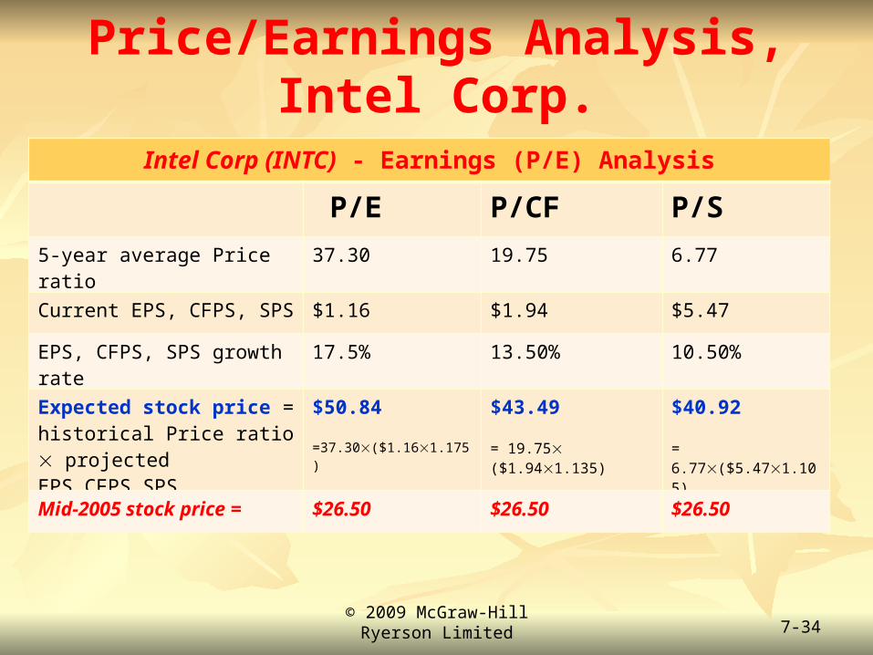
Price/Earnings Analysis, Intel Corp.

Intel Corp (INTC) - Earnings (P/E) Analysis

Intel Corp (INTC) - Earnings (P/E) Analysis

P/E P/CF P/S

5-year average Price ratio 37.30 19.75 6.77

Current EPS, CFPS, SPS $1.16 $1.94 $5.47

EPS, CFPS, SPS growth rate 17.5% 13.50% 10.50%

Expected stock price = historical Price ratio projected EPS,CFPS,SPS

$50.84

=37.30($1.161.175)

$43.49

= 19.75 ($1.941.135)

$40.92

= 6.77($5.471.105)

Mid-2005 stock price = $26.50 $26.50 $26.50

7-35

The McGraw-Hill Company Analysis

Figure 7.2

The next few slides contain a financial analysis of the McGraw-Hill Company, using data from the Value Line Investment Survey.



Based on the CAPM, k = 3.1% + (.80 9%) = 10.3% Retention ratio = 1 – $.66/$2.65 = .751 Sustainable g = .751 23% = 17.27% Because g > k, the constant growth rate model cannot be

used. (We would get a value of -$11.10 per share)


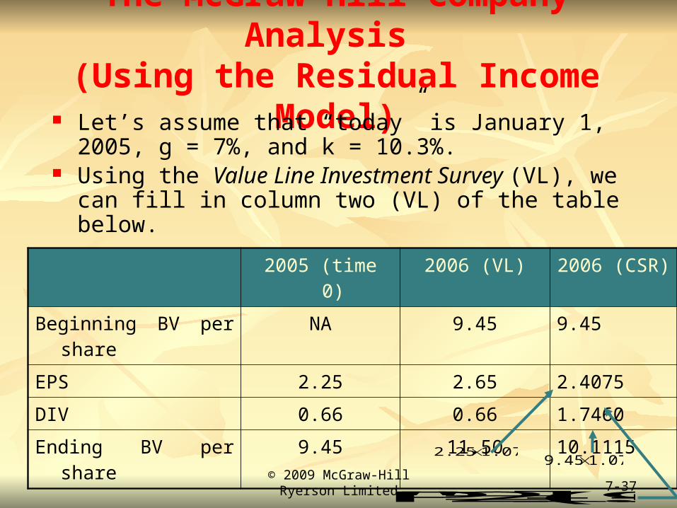
The McGraw-Hill Company Analysis (Using the Residual Income Model)

Let’s assume that “today” is January 1, 2005, g = 7%, and k = 10.3%.

Using the Value Line Investment Survey (VL), we can fill in column two (VL) of the table below.

2005 (time 0) 2006 (VL) 2006 (CSR)

Beginning BV per share NA 9.45 9.45

EPS 2.25 2.65 2.4075

DIV 0.66 0.66 1.7460

Ending BV per share 9.45 11.50 10.1115

1.072.251.079.45

9.45) - (10.1115-2.4075 Plug""

7-38


Using the CSR assumption:

Using Value Line numbers for EPS1=$2.65, B1=$11.50B0=$9.45; and using the actual change in book value instead of an estimate of the new book value, (i.e., B1-B0 is = B0 x k)

$52.91.P

.07.103

.103$9.45.07)(1$2.25$9.45P

gk

kBg)(1EPSBP

0

0

0000

$27.63P

.07.103

9.45)-($11.50$2.65$9.45P

gk

kBg)(1EPSBP

0

0

0000

Stock price at the time = $47.04.What can we say?



Table 7.4

Quick calculations used: P/CF = P/E EPS/CFPS

P/S = P/E EPS/SPS


Useful Internet Sites

• www.nyssa.org (the New York Society of Security Analysts)• www.valueline.com (the home of the Value Line Investment Survey)

• Websites for the companies analyzed in this chapter:• www.aep.com • www.americanexpress.com • www.pepsico.com • www.starbucks.com • www.sears.com • www.intel.com • www.disney.go.com • www.mcgraw-hill.com

http://www.nyssa.org/

http://www.valueline.com/

http://www.aep.com/

http://www.americanexpress.com/

http://www.pepsico.com/

http://www.starbucks.com/

http://www.sears.com/

http://www.intel.com/

http://www.disney.go.com/

http://www.mcgraw-hill.com/

Documents

© 2009 McGraw-Hill Ryerson Limited 7-1 Chapter 7 Common Stock Valuation CHAPTER OUTLINE Security analysis Security analysis The dividend discount model