© 2004 Goodrich, Tamassia Hash Tables1 0 1 2 3 4 451-22-0004 981-10-0002 025-61-0001

© 2004 Goodrich, Tamassia Hash Tables 1

Hash Tables

01234 451-22-0004

981-10-0002

025-61-0001


Recall the Map ADTMap ADT methods: get(k): if the map M has an entry with key k,

return its assoiciated value; else, return null put(k, v): insert entry (k, v) into the map M;

if key k is not already in M, then return null; else, return old value associated with k

remove(k): if the map M has an entry with key k, remove it from M and return its associated value; else, return null

size(), isEmpty() keys(): return an iterator of the keys in M values(): return an iterator of the values in

M


Hash Functions and Hash Tables

A hash function h maps keys of a given type to integers in a fixed interval [0, N1]

Example:h(x) x mod N

is a hash function for integer keysThe integer h(x) is called the hash value of key x

A hash table for a given key type consists of Hash function h Array or Vector (called “table”) of size N

When implementing a map with a hash table, the goal is to store item (k, o) at index i h(k)


Example

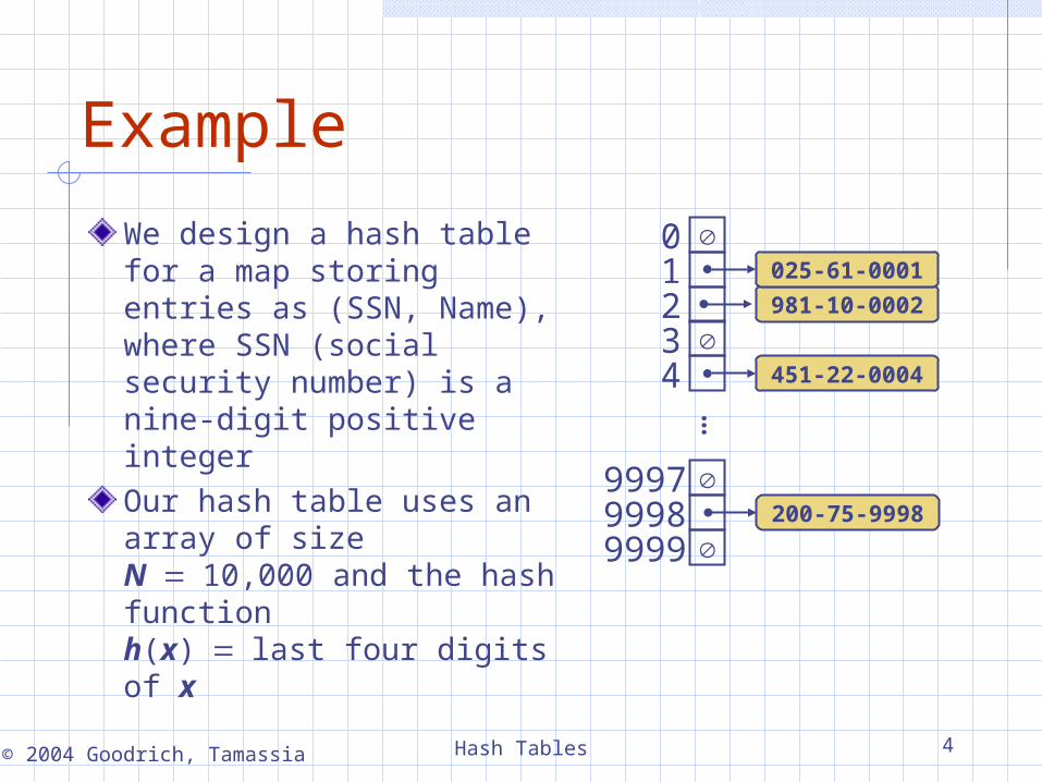
We design a hash table for a map storing entries as (SSN, Name), where SSN (social security number) is a nine-digit positive integerOur hash table uses an array of size N10,000 and the hash functionh(x)last four digits of x

01234

999799989999

…451-22-0004

981-10-0002

200-75-9998

025-61-0001


Hash Functions

A hash function is usually specified as the composition of two functions:Hash code: h1: keys integers

Compression function: h2: integers [0, N1]

The hash code is applied first, and the compression function is applied next on the result, i.e.,

h(x) = h2(h1(x))

The goal of the hash function is to “disperse” the keys in a random way


Compression Functions

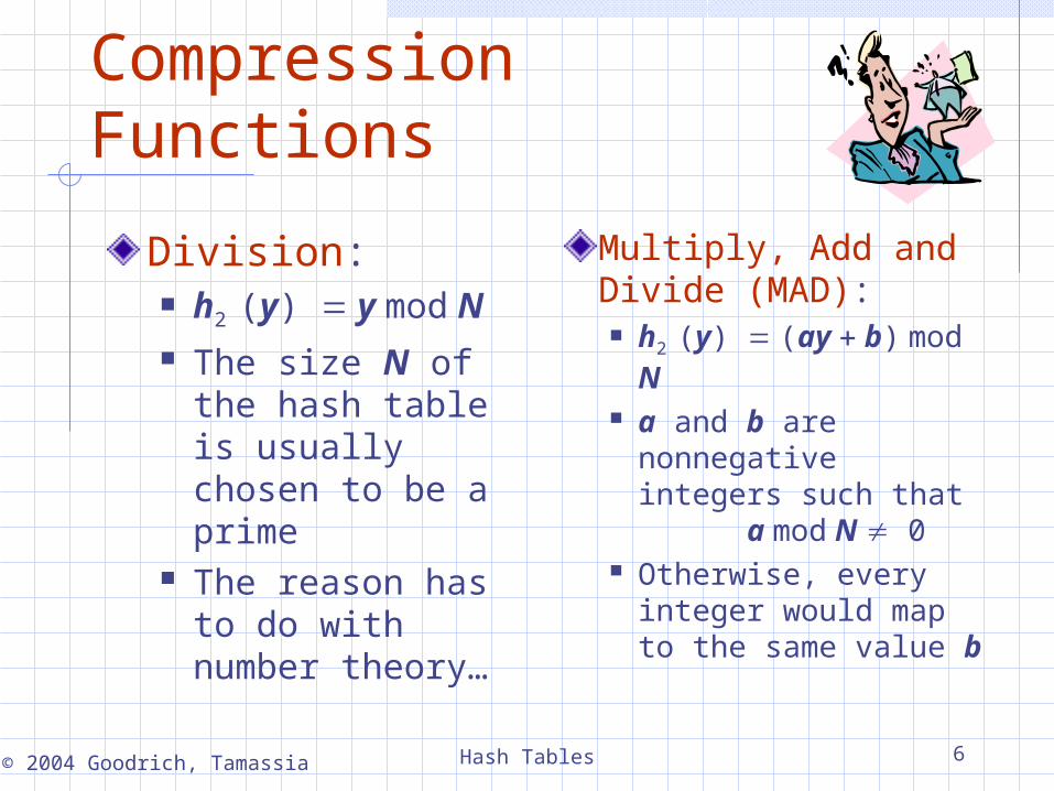
Division: h2 (y) y mod N The size N of the

hash table is usually chosen to be a prime

The reason has to do with number theory…

Multiply, Add and Divide (MAD): h2 (y) (ay b) mod N a and b are

nonnegative integers such that

a mod N 0 Otherwise, every

integer would map to the same value b


Collision Handling

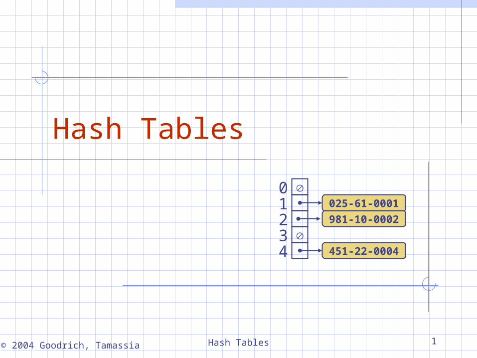
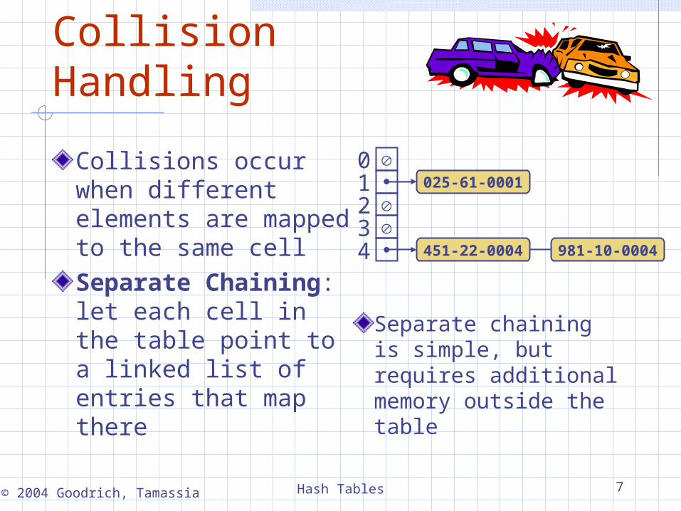
Collisions occur when different elements are mapped to the same cellSeparate Chaining: let each cell in the table point to a linked list of entries that map there

Separate chaining is simple, but requires additional memory outside the table

01234 451-22-0004 981-10-0004

025-61-0001


Map Methods with Separate Chaining used for Collisions

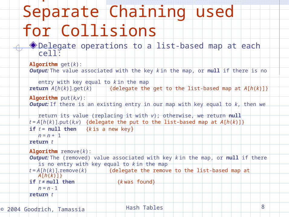
Delegate operations to a list-based map at each cell:

Algorithm get(k):Output: The value associated with the key k in the map, or null if there is no

entry with key equal to k in the mapreturn A[h(k)].get(k) {delegate the get to the list-based map at A[h(k)]}

Algorithm put(k,v):Output: If there is an existing entry in our map with key equal to k, then we

return its value (replacing it with v); otherwise, we return nullt = A[h(k)].put(k,v) {delegate the put to the list-based map at A[h(k)]}if t = null then {k is a new key}

n = n + 1return t

Algorithm remove(k):Output: The (removed) value associated with key k in the map, or null if there

is no entry with key equal to k in the mapt = A[h(k)].remove(k) {delegate the remove to the list-based map at A[h(k)]}if t ≠ null then {k was found}

n = n - 1return t


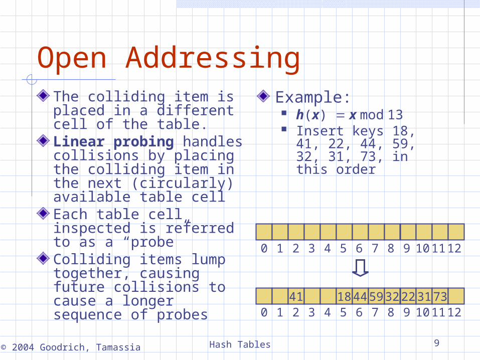
Open AddressingThe colliding item is placed in a different cell of the table.Linear probing handles collisions by placing the colliding item in the next (circularly) available table cellEach table cell inspected is referred to as a “probe”Colliding items lump together, causing future collisions to cause a longer sequence of probes

Example: h(x) x mod 13 Insert keys 18, 41, 22,

44, 59, 32, 31, 73, in this order

0 1 2 3 4 5 6 7 8 9 10 11 12

41 18445932223173 0 1 2 3 4 5 6 7 8 9 10 11 12


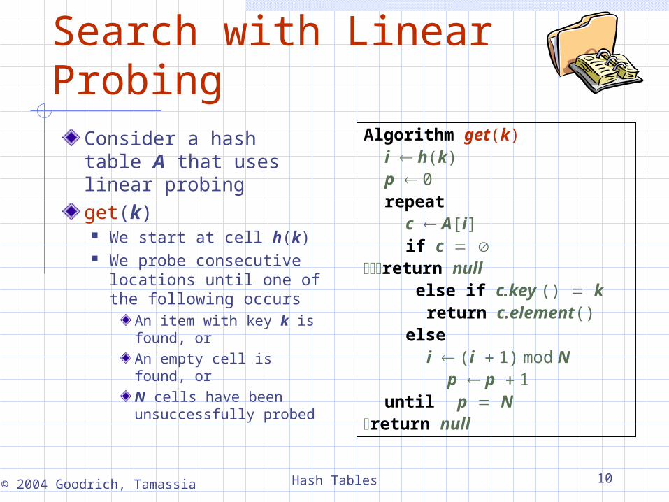
Search with Linear ProbingConsider a hash table A that uses linear probingget(k)

We start at cell h(k) We probe consecutive

locations until one of the following occurs

An item with key k is found, orAn empty cell is found, orN cells have been unsuccessfully probed

Algorithm get(k)i h(k)p 0repeat

c A[i]if c

return null else if c.key () k

return c.element()else

i (i 1) mod Np p 1

until p Nreturn null


Updates with Linear Probing

To handle insertions and deletions, we introduce a special object, called AVAILABLE, which replaces deleted elementsremove(k)

We search for an entry with key k If such an entry (k, o) is found, we replace it with the special item AVAILABLE and we return element oElse, we return null

put(k, o) We throw an

exception if the table is full

We start at cell h(k) We probe

consecutive cells until one of the following occurs

A cell i is found that is either empty or stores AVAILABLE, orN cells have been unsuccessfully probed

We store entry (k, o) in cell i


Double HashingDouble hashing uses a secondary hash function d(k) and handles collisions by placing an item in the first available cell of the series

(i jd(k)) mod N for j 0, 1, … , N 1The secondary hash function d(k) cannot have zero valuesThe table size N must be a prime to allow probing of all the cells

Common choice of compression function for the secondary hash function: d2(k) q (k mod q)

where q N q is a prime

The possible values for d2(k) are

1, 2, … , q


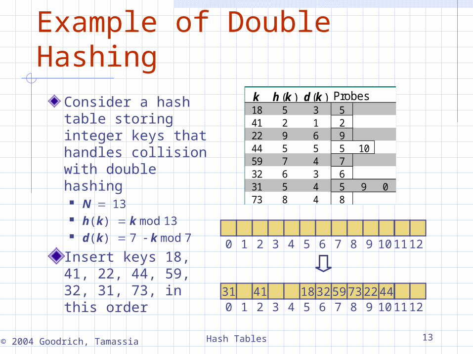
Consider a hash table storing integer keys that handles collision with double hashing

N13 h(k) k mod 13 d(k) 7 k mod 7

Insert keys 18, 41, 22, 44, 59, 32, 31, 73, in this order

Example of Double Hashing

0 1 2 3 4 5 6 7 8 9 10 11 12

31 41 183259732244 0 1 2 3 4 5 6 7 8 9 10 11 12

k h (k ) d (k ) Probes18 5 3 541 2 1 222 9 6 944 5 5 5 1059 7 4 732 6 3 631 5 4 5 9 073 8 4 8


Performance of Hashing

In the worst case, searches, insertions and removals on a hash table take O(n) timeThe worst case occurs when all the keys inserted into the map collideThe load factor nN affects the performance of a hash tableAssuming that the hash values are like random numbers, it can be shown that the expected number of probes for an insertion with open addressing is

1 (1 )

The expected running time of all the dictionary ADT operations in a hash table is O(1) In practice, hashing is very fast provided the load factor is not close to 100%When the load gets too high, we can rehash….Applications: very numerous, e.g. computing frequencies.

Documents

© 2004 Goodrich, Tamassia Hash Tables1 0 1 2 3 4 451-22-0004 981-10-0002 025-61-0001