© 2001 Martin Culpepper - MIT OpenCourseWare · Design of Constraints in Precision Systems Background History Reasons Requirements Problems Classes of Constraint Kinematic Quasi-Kinematic

© 2001 Martin Culpepper

Design of Constraints in Precision Systems Background

� History

� Reasons

� Requirements

� Problems

Classes of Constraint

� Kinematic

� Quasi-Kinematic

� Variable Geometry

� Partial/Compliance

Hardware/discussion time

Elastic Averaging will be done next lecture



Elastic Averaging

Non-Deterministic

Pinned Joints

No Unique Position

Kinematic Couplings

Kinematic Constraint

Flexural Kin. Couplings

Kinematic Constraint

Quasi-Kinematic Couplings

Near Kinematic Constraint

Common Coupling Methods

Perspective: What the coupling designer faces…

APPLICATION

Fiber Optics

Optical Resonators

Large array telescopes

Automotive

Problems due to strain affects

� Thermal Affects

� Gravity

� Stress Relief

� Loads

SYSTEM SIZE

Meso

Meso

60 ft diam.

3 ft

Air, hands, sunlight Sagging Time variable assemblies Stiffness

REQ’D PRECISION

Nano

Nano

Angstrom

1 micron

Problems due to sub-optimal designers

� Competing cost vs performance

� Automotive (no temperature control, large parts, resistance to change)


General Service Requirements & Applications

Ideal couplings:

� Inexpensive

� Accurate & Repeatable

� High Stiffness

� Handle Load Capacity

� Sealing Interfaces

� Well Damping

Example Applications:

� Grinding

� Optic Mounts

� Robotics

� Automotive

Sensitivity

� What are the sensitive directions?!?!?!?!?


Couplings Are Designed as Systems

You must know what is going on (loads, environment, thermal)!

Shoot for determinism or it will “suck to be you”

CouplingSystem

Force

Disturbance

Displacement

Disturbance

Material

Property

Disturbance

Geometry

Disturbance

Inputs•Force

•Displacement

Desired Outputs •Desired Location

Actual Outputs•Actual Location

Error

Kinematics Material

Geometry Others


The good, the bad, the ugly….


Defining Constraint

Penalties for over constraintClever use of constraint© 2001 Martin Culpepper

Exact Constraint (Kinematic) Design

Exact Constraint: Number of constraint points = DOF to be constrained

These constraints must be independent!!!

Assuming couplings have rigid bodies, equations can be written todescribe movements

Design is deterministic, saves design and development $

KCs provide repeatability on the order of parts’ surface finish

� ¼ micron repeatability is common

� Managing contact stresses are the key to success


Making Life Easier

“Kinematic Design”, “Exact Constraint Design”…..the issues are:

� KNOW what is happening in the system

� Manage forces and deflections

� Minimize stored energy in the coupling

� Know when “Kinematic Design” should be used

� Know when “Elastic Averaging” should be used (next week)

Boyes ClampKelvin Clamp© 2001 Martin Culpepper

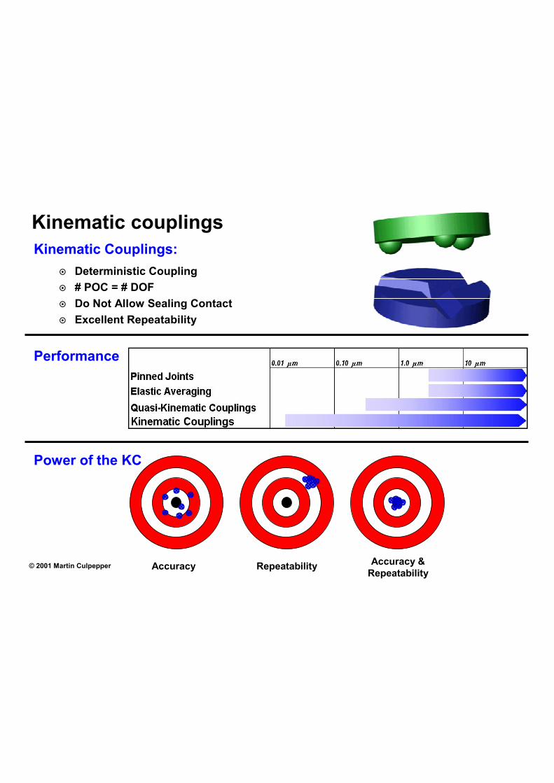
Kinematic couplings Kinematic Couplings:

� Deterministic Coupling

� # POC = # DOF

� Do Not Allow Sealing Contact

� Excellent Repeatability

Performance

Power of the KC

Accuracy &© 2001 Martin Culpepper Accuracy Repeatability

Repeatability

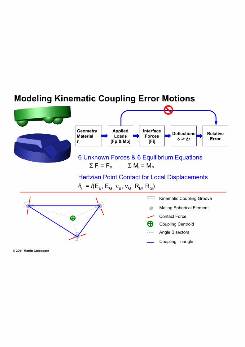
Modeling Kinematic Coupling Error Motions

InterfaceForces

[Fi]

AppliedLoads

[Fp & Mp]

Deflectionsδδδδ -> ∆∆∆∆r

RelativeError

GeometryMaterialni

6 Unknown Forces & 6 Equilibrium Equations

Σ Fi = FP Σ Mi = MP

Hertzian Point Contact for Local Displacements

δi = f(EB, EG, νB, νG, RB, RG)

Kinematic Coupling Groove

Mating Spherical Element

Contact Force

Coupling Centroid

Angle Bisectors

Coupling Triangle


δδδ δδδ δδδ εεε εεε εεε

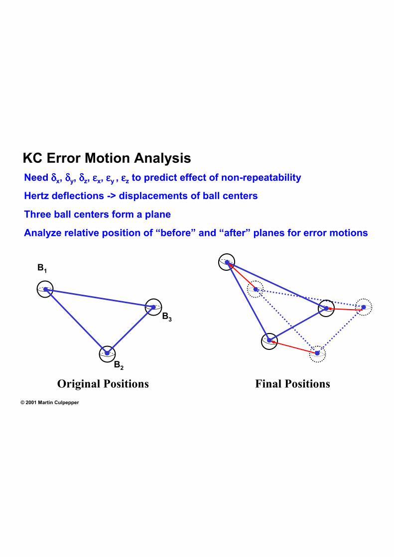
KC Error Motion Analysis

Need δx, δy, δz, εx, εy , εz to predict effect of non-repeatability

Hertz deflections -> displacements of ball centers

Three ball centers form a plane

Analyze relative position of “before” and “after” planes for error motions

B1

B3

B2

Original Positions Final Positions


δδδ

Kinematic Couplings and Distance of Approach How do we characterize motions of the ball centers?

δn = distance of approach

Initial Position of

Ball’s Far Field Point

Initial Contact Point

Final Position of

Ball’s Far Field Point

δδδδr

δδδδz

δδδδn

δδδδl

r

z

l

n

Final True Groove’s

Far Field Point

Initial Position of

Groove’s Far Field Point

Final Contact Point

Max τ

© 2001 Martin Culpepper Max shear stress occurs below surface, in the member with larges R

δδδ

ννν

Contact Mechanics – Hertz Contact Heinrich Hertz – 1st analytic solution for “near” point contact

KC contacts are modeled as Hertz Contacts

Enables us to determine stress and distance of approach, δn

Radii Ronemaj 1.00E+06

Ronemin 0.06250

Rtwomaj 0.25000

Rtwomin -0.06500

Applied load F 13

Phi (degrees) 0

Max contact stress 10,000

Elastic modulus Eone 3.00E+07

Elastic modulus Etwo 4.40E+05

Poisson's ratio vone 0.3

Poisson's ratio vtwo 0.3

Equivalent modulus Ee 4.77E+05

Equivalent radius Re 0.2167

Contact pressure 12,162

Stress ratio (must be less than 1) 1.22

Deflection at the one contact interface

Deflection (µunits) 829

F

F

Load ∆ = 2 δn

Modulus

ν Ratio

Stress

Deflection


θθθ φφφ

Minor Contact Axis

Major ContactAxis

Distance of Approach

Contact Pressure

β 3FRe2Ee

1/3c = α 3FRe

2Ee

1/3

Key Hertz Physical Relations

Equivalent radius and modulus:Re = 1

1 + 1 + 1 + 1 Ee =2

12

R1major R1minor R2major R2minor1 -

E1

η1 +1 -

E2

η2

cos(θ) function (φ is the angle between the planes of principal curvature of the two bodies)

2cosθ = Re

1 - 1 2+ 1 - 1

R1major R1minor R2major R2minor

+ 2 1 - 1 1 - 1 cos2φ1/2

R1major R1minor R2major R2minor

Solution to elliptic integrals estimated with curve fitsα = 1.939e-5.26θ + 1.78e-1.09θ + 0.723/θ + 0.221

β = 35.228e-0.98θ - 32.424e-1.0475θ + 1.486θ - 2.634

λ = -0.214e-4.95θ - 0.179θ2 + 0.555θ + 0.319

Contact Pressure Distance of Approach

Major ContactAxis

Minor Contact Axis

q = 3F2πcd

≈ 1.5σtensile for metals δ = λ 2F2

3ReEe2

1/3

c = α 3FRe2Ee

1/3β 3FRe

2Ee

1/3


KEY Hertz Relations

Contact Pressure is proportional to:

� Force to the 1/3rd power

� Radius to the –2/3rd power

� Modulus to the 2/3rd power

Distance of approach is proportional to:


� Radius to the –1/3rd power

� Modulus to the –2/3rd power

Contact ellipse diameter is proportional to:


� Radius to the 1/3rd power

� Modulus to the –1/3rd power

DO NOT ALLOW THE CONTACT ELLIPSE TO BE WITHIN ONE DIAMETER OF THE EDGE OF A SURFACE!


∆∆ ∆∆ ∆∆

Calculating Errors Motions in Kinematic Couplings Motion of ball centers -> Centroid motion in 6 DOF -> ∆x, ∆y, ∆z at X, Y, Z∆ ∆ ∆

� Coupling Centroid Translation Errors

⎛ δ δ δ ⎞ L + L + L1ζ 2ζ 3ζ 1c 2c 3cδ ⎜ + + ⎟⋅ζc

L L L 3⎝ 1c 2c 3c ⎠

� Rotations

δ δ δz1 z2 z3ε cos θ⋅ cos θ⋅+ cos θ⋅+( ) ( ) ( )x 23 31 12

L 23, L 31, L 12,1 2 3

δ δ δz1 z2 z3ε sin θ⋅ sin θ⋅+ sin θ⋅+( ) ( ) ( )y 23 31 12

L 23, L 31, L 12,1 2 3

α B1 δ 1⋅ B2 δ 2⋅+( 2β B1 δ 1⋅ B2 δ 2⋅+( 2

+α ) β ) ε ε+ ε+z1 z2 z3

x1 x c−( 2y 1 y c−( 2+) )

ε zε SIGN α δ⋅ α δ⋅−⋅ ( )z1 B1 1 B2 2 3

� Error At X, Y, Z (includes translation and sine errors)

− −⎛ ∆ x ⎞ ⎛ 1 −ε z ε y δ x ⎞ ⎛ X xc ⎞ ⎛ X xc ⎞⎜ ⎟ ⎜ ⎟ ⎜ ⎟ ⎜ ⎟

∆ ε 1 ε− δ Y y− Y y−⎜ y ⎟ ⎜ z x y ⎟ ⎜ c ⎟ ⎜ c ⎟⋅ −⎜ ⎟ ⎜ ⎟ ⎜ ⎟ ⎜ ⎟Z z− Z z−∆ ε− ε 1 δ c cz y x z⎜ ⎟ ⎜ ⎟ ⎜ ⎟ ⎜ ⎟⎝ 1 ⎠ ⎝ 0 0 0 1 ⎠ ⎝ 1 ⎠ ⎝ 1 ⎠


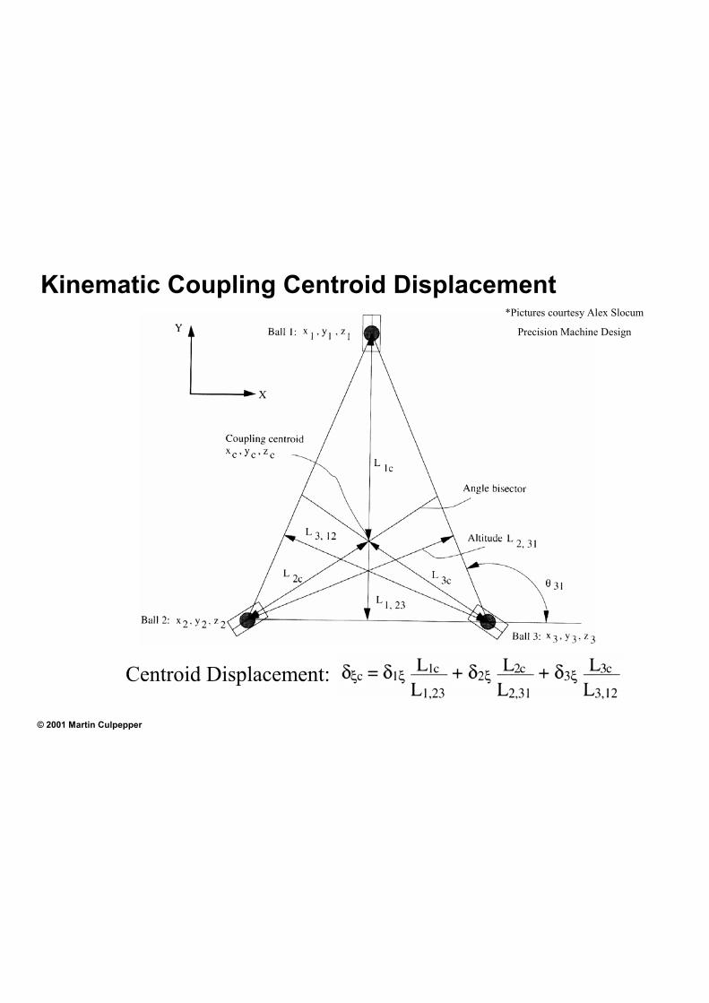
Kinematic Coupling Centroid Displacement ex*Pictures courtesy Al

Precision Machine D

Slocum

esign

Centroid Displacement:


General Design Guidelines

1. Location of the coupling plane is important to avoid sine errors

2. For good stability, normals to planes containing contact for vectors should bisect angles of coupling triangle

3. Coupling triangle centroid lies at center circle that coincides with the three ball centers

4. Coupling centroid is at intersection of angle bisectors

5. These are only coincident for equilateral triangles

6. Mounting the balls at different radii makes crash-proof

7. Non-symmetric grooves make coupling idiot-proof


Kinematic Coupling Stability Theory

Poor Design

Good Design

*Pictures courtesy Alex Slocum

Precision Machine Design


Sources of Errors in KCs

Thermal

Surface Errors

CouplingSystem

Force

Disturbance

Displacement

Disturbance

Material

Property

Disturbance

Geometry

Disturbance

Inputs•Force

•Displacement

Desired Outputs •Desired Location

Actual Outputs•Actual Location

Error

Kinematics Material

Geometry Others

Finish

Error Loads

Preload Variation


µµµ

µµµ

Problems With Physical Contact (and solutions) Surface topology (finish):

� 50 cycle repeatability ~ 1/3 µm Ra

BA

λλλλ

Mate n

BA

λλλλ

Mate n + 1

� Friction depends on surface finish!

� Finish should be a design spec

� Surface may be brinelled if possible

Wear and Fretting:

� High stress + sliding = wear

� Metallic surfaces = fretting

� Use ceramics if possible (low µ and high strength)

� Dissimilar metals avoids “snowballing”

Wear

on

Gro

ove

Friction:

� Friction = Hysteresis, stored energy, overconstraint

� Flexures can help (see right)

� Lubrication (high pressure grease) helps

- Beware settling time and particles

� Tapping can help if you have the “magic touch”

Ball in V-Groove with Elastic Hinges© 2001 Martin Culpepper

Experimental Results –Repeatability & Lubrication


Number of Trials

Radial Repeatability (Unlubricated)2

0

Dis

pla

cem

en

t,µµ µµm

600

Number of Trials

Radial Repeatability (Lubricated)

600

Dis

pla

cem

en

t,µµ µµm

2

0

Practical Design of Kinematic Couplings Design

� Specify surface finish or brinell on contacting surfaces

� Normal to contact forces bisect angles of coupling triangle!!!

Manufacturing & Performance

� Repeatability = f (friction, surface, error loads, preload variation, stiffness)

� Accuracy = f (assembly) unless using and ARKC

Precision Balls (ubiquitous, easy to buy)

� Baltec sells hardened, polished kinematic coupling balls or…..

Grooves (more difficult to make than balls)

� May be integral or inserts. Inserts should be potted with thin layer of epoxy

Materials

� Ceramics = low friction, high stiffness, and small contact points

� If using metals, harden

� Use dissimilar materials for ball and groove

Preparation and Assembly

� Clean with oil mist

� Lubricate grooves if needed


Example: Servo-Controlled Kinematic Couplings

Location & automatic leveling of precision electronic test equipment

Teradyne has shipped over 500 systems


Example: Canoe-Ball Kinematic Interface Element The “Canoe Ball” shape is the secret to a highly repeatable design

� It acts like a ball 1 meter in diameter

� It has 100 times the stiffness and load capacity of a normal 1” ball

Large, shallow Hertzian zone is very (i.e. < 0.1 microns) repeatable


µµ µµµ µ

µµµ

µµµ

µµµ

µµµ

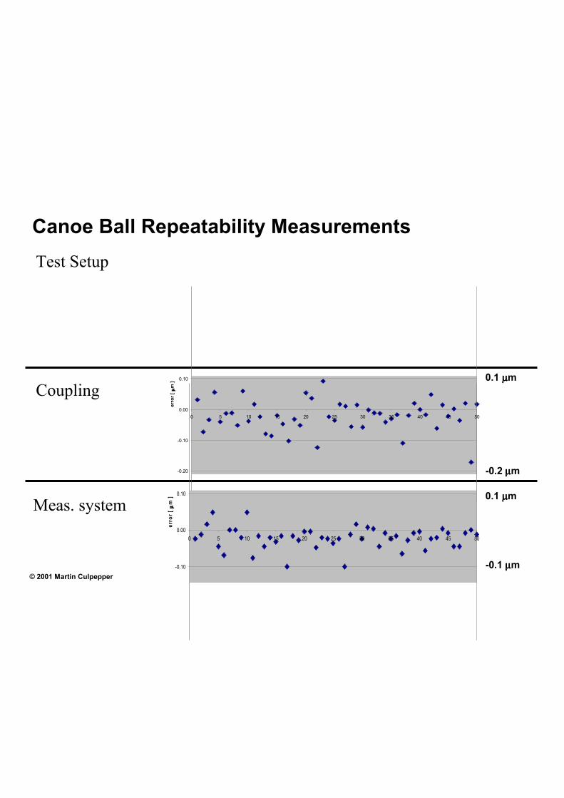
Canoe Ball Repeatability Measurements

Test Setup

0.1 µm

Coupling0.10

err

or

[ µm

]

err

or

[ µm

]

0 5 10 15 20 25 30 35 40 45 50

0.00

-0.10

-0.20 -0.2 µm

Meas. system 0.10

0 5 10 15 20 25 30 35 40 45 50

0.1 µm

0.00

-0.10 -0.1 µm© 2001 Martin Culpepper

Why do it the easy way when you can do it the lazy way?


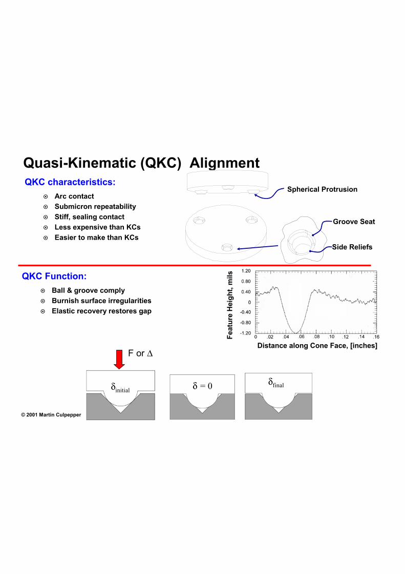
Quasi-Kinematic (QKC) Alignment QKC characteristics:

� Arc contact

� Submicron repeatability

� Stiff, sealing contact

� Less expensive than KCs

� Easier to make than KCs

Spherical Protrusion

Groove Seat

Side Reliefs

QKC Function:

� Ball & groove comply

� Burnish surface irregularities

� Elastic recovery restores gap

Distance along Cone Face, [inches]F or ∆

Featu

re H

eig

ht,

mil

s

δinitialδ = 0

δfinal


Details of QKC Element Geometry PAIRS OF QKC ELEMENTS

+ OR +


BOLT

BEDPLATE

BLOCK

PEG

ASSEMBLED JOINTTYPE 2 GROOVE MFG.

CAST FORM TOOL FINISHED

+ =

QKC Methods vs Kinematic Method

x

y

Relief

Components and Definitions

Cone Seat

Ball

Groove Surface

Peg Surface

Relief

Contact Point

Force Diagrams


ResultantForces[ni & Fi]

AppliedLoads

[Fp & Mp]

Deflectionsδδδδ -> ∆∆∆∆r

RelativeError

GeometryMaterial

Modeling QKC Stiffness

24 Unknowns & 7 Eqxns.

QKC Model Geometry

Material

Displacements

Contact Stiffnessfn(δδδδn)

Force/Torque

Stiffness


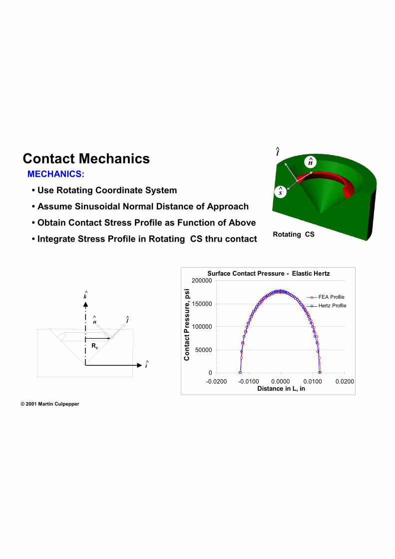
Contact MechanicsMECHANICS:

• Use Rotating Coordinate System

• Assume Sinusoidal Normal Distance of Approach

• Obtain Contact Stress Profile as Function of Above

• Integrate Stress Profile in Rotating CS thru contact

^k

n l^

Rc

^

^i

Rotating CS

n

l

s

^

^

Surface Contact Pressure - Elastic Hertz

0

50000

100000

150000

200000

-0.0200 -0.0100 0.0000 0.0100 0.0200Distance in L, in

Co

nta

ct P

res

su

re,p

si

FEA Profile

Hertz Profile


µµµ

µµµ

µµµ

Example: Duratec Assembly

Characteristics:

• Ford 2.5 & 3.0 L V6 10 µm

• > 300,000 Units / Year

• Cycle Time: < 30 s

Coupling + Others 5 µm

Process 0 µm

Rough Error Budget


Example: Assembly of Duratec Block and Bedplate

COMPONENTS

Block Bedplate

C B Halves

Block

Bedplate

Assembly Bolts

r

a

JR

δδδδe

JL

Block Bore

Bedplate Bore

CL

CL

δδδδe MAX = 5 microns

ERRORASSEMBLY


Bearing Assemblies in Engines

Bedplate Main

Bearing Half

Block Main

Bearing Half Crank Shaft Journal

Block

Main Bearing

Bedplate

Crank Shaft

Piston

Halves


Results of Duratec QKC Research MANUFACTURING:Engine Manufacturing Process With Pinned Joint

Op. #10

• Mill Joint Face

• Drill/Bore 16 Holes

• Drill Bolt Holes

Op. #30


Op. #50

• Press in 8 Dowels

• Assemble

• Load Bolts

• Torque Bolts

Op. #100

• Semi-finish crank bores

• Finish crank bores

Modified Engine Manufacturing Process Using Kinni-Mate Coupling

Op. #10 Op. #30


Op. #50

• Press 3 Pegs in BP

• Assemble

• Load Bolts

• Torque Bolts

Op. #100

• Mill Joint Face • Semi-finish crank bores

• Drill/Bore 3 Peg Holes • Finish crank bores

• Drill Bolt Holes & Form3 Conical Grooves

DESIGN:


Engine Assembly Performance Axial

JL Cap Probe

Sensitive1st Block Fixture CMM Head

Bedplate Fixture

Bedplate

JR Cap Probe

Axial Cap Probe

2nd Block Fixture

QKC Error in Sensitive Direction

-2.0

-1.5

-1.0

-0.5

0.0

0.5

1.0

1.5

2.0

0 2 4 5 6 8

Trial #

δ c,

mic

ron

s

JL

JR

1 3 7

QKC Error in Axial Direction

-2.0

-1.5

-1.0

-0.5

0.0

0.5

1.0

1.5

2.0

0 6

Trial #

δ a,

mic

ron

s

Max x Dislacement

54321 7

(Range/2)|AVG = 0.65 µm (Range/2) = 1.35 µm


8

Documents

© 2001 Martin Culpepper - MIT OpenCourseWare · Design of Constraints in Precision Systems Background History Reasons Requirements Problems Classes of Constraint Kinematic Quasi-Kinematic