JSS Journal of Statistical SoftwareOctober 2010, Volume 36, Issue 13. http://www.jstatsoft.org/

Interactive Teaching Tools for Spatial Sampling

Adrian W. BowmanUniversity of Glasgow

Iain GibsonUniversity of Glasgow

E. Marian ScottUniversity of Glasgow

Ewan CrawfordUniversity of Glasgow

Abstract

The statistical analysis of data which is measured over a spatial region is well es-tablished as a scientific tool which makes considerable contributions to a wide varietyof application areas. Further development of these tools also remains a central part ofthe research scene in statistics. However, understanding of the concepts involved oftenbenefits from an intuitive and experimental approach, as well as a formal description ofmodels and methods. This paper describes software which is intended to assist in thisunderstanding. The role of simulation is advocated, in order to explain the meaning ofspatial correlation and to interpret the parameters involved in standard models. Realisticscenarios where decisions on the locations of sampling points in a spatial setting are re-quired are also described. Students are provided with a variety of sampling strategies andinvited to select the most appropriate one in two different settings. One involves watersampling in the lagoon of the Mururoa Atoll while the other involves sea bed sampling ina Scottish firth. Once a student has decided on a sampling strategy, simulated data areprovided for further analysis. This extends the range of teaching activity from the analysisof data collected by others to involvement in data collection and the need to grapple withissues of design. It is argued that this approach has significant benefits in learning.

The software which implements these tools is built on existing R packages, using rpanelcontrols for the geoR geostatistical simulation and modelling tools. The operation andconstruction of the software are described in detail. The software is made available asadditional functions rp.geosim, rp.mururoa and rp.firth in the rpanel package.

Keywords: interactive graphics, graphical user interface, learning, sampling, simulation, spa-tial statistics, R, teaching.

1. Introduction

The statistical analysis of spatial data has been a major growth area of statistical research for

2 Interactive Teaching Tools for Spatial Sampling

around three decades and it continues to occupy a place at the very heart of current research.The need to adapt statistical analysis to spatial structures has generated very importantmethodological innovations. On the other hand, the existence of appropriate spatial methodshas had enormously significant impact on a wide variety of application areas, from image pro-cessing to environmental problems. Cressie (1993) gives an authoritative and comprehensiveoverview of spatial concepts and techniques while a wide variety of more recent texts offerdifferent perspectives on the subject and address important application areas, particularlyenvironmental science (Webster and Oliver 2001; Piegorsch and Bailer 2005; Barnett 2006;Diggle and Ribiero 2007).

The concepts associated with spatial variation, and in particular spatial correlation, need to befirmly understood if spatial analyses are to be properly implemented and interpreted. Whenthese concepts are met for the first time, they are not always easy to grasp, particularlyfor those whose background lies in application areas where quantitative traditions are notstrong. However, even those who are able to approach the topic from a strong backgroundin the mathematical sciences often benefit from opportunities to develop a more intuitiveunderstanding to complement the theory.

Appropriate use of software can make substantial contributions towards these aims. A numberof excellent packages to fit spatial models are now available and the ability to use these onrelevant data allows a shift of focus from the algorithmic to the conceptual. An importantexample implemented in the R system for statistical computing (R Development Core Team2010) is the geoR package (Ribeiro and Diggle 2001) which provides a wide variety of toolsfor the analysis of geostatistical data. This makes use in turn of the sp classes and methods(Pebesma and Bivand 2005; Bivand, Pebesma, and Gomez-Rubio 2008) for spatial data andthe RandomFields (Schlather 2009) package for the simulation of data from random fields.

While direct use of analysis packages enables students to engage with real applications, thereremains scope for software whose role is to explain the meaning of spatial models and to allowstudents to explore standard concepts such as the meaning of variation in a spatial setting.The ShowModels function in the RandomFields package, described by Schlather (2001), is agood example of what can be achieved with standard mouse-click interaction on an R graphicswindow. However, the advent of graphical user interface (GUI) software in R greatly extendsthe scope for the construction and use of interactive tools. There are now many differentsystems to construct GUI controls, such as iplots (Urbanek and Theus 2003), JGR (Helbig,Urbanek, and Fellows 2010), RGtk2 (Lawrence and Temple Lang 2010) and gWidgets (Verzani2007). The particular niche occupied by the rpanel package (Bowman, Crawford, Alexander,and Bowman 2007), which in turn is built on the tcltk system (Dalgaard 2001), is expressedin the aim to make the addition of interactive graphical controls as simple as possible. Thispaper reports on the the use of rpanel to create software which allow students to engagegraphically with spatial concepts. It is available from the Comprehensive R Archive Networkat http://CRAN.R-project.org/package=rpanel.

The role of simulation is discussed in Section 2, where software to provide interactive controlof model parameters and displays is described. Sections 3 and 4 discuss two scenarios wheredata are to be sampled from a spatial region. Students are required to make a decision onhow this sampling should be conducted, with the software providing a variety of options, andsome simple analysis of the collected data. Some final discussion is given in Section 5. Issuesof software design are discussed in an appendix.

Journal of Statistical Software 3

2. Simulation of spatial data

Simulation provides a very natural tool to promote an intuitive understanding of randomvariation in a variety of settings, simply by viewing repeated realizations of data. For spatialdata, a helpful starting point is the simulation of random surfaces which are generated bya Gaussian process. If, for simplicity, the mean value is set to 0, then the process can bedefined over a spatial region by the covariance function C(s, t), where s and t denote spatiallocations. When the process is (weakly) stationary, C is a function only of h = ||s − t||, thedistance between the two spatial locations. The material described in this paper uses theMatern covariance function

C(h) =σ2

2κ−1Γ(κ)

(h

φ

)κ

Kκ

(h

φ

),

where Kκ(x) denotes the modified Bessel function of the third kind of order κ. This offersa flexible family of covariance functions with a degree of control of shape expressed in theparameter κ. For example, the standard exponential model is obtained by setting κ = 0.5.Since many covariance functions have broadly similar shapes, it is the role of the variance(σ2) and correlation range (φ) parameters which are of most interest. However, in the pa-rameterization shown above, the range is also directly affected by κ. This can be remediedby adopting the parameterization of Handcock and Wallis (1994), defined by φ = θ/(2

√κ),

which gives the new range parameter θ a clear interpretation, unaffected by the setting of κ.This parameterization has been adopted here.

For visualization, the random surface generated by the Gaussian process can be evaluated ata fine grid of spatial locations. A simple approach is to construct the covariance matrix Σwhose (i, j)th element contains C evaluated at grid points i and j. A Cholesky, or equivalent,decomposition of Σ provides a matrix which, when multiplied by a vector of independentstandard normal random variables, produces a vector of data whose covariance matrix is Σ.This approach can be very inefficient when large samples are involved but a variety of othercomputational approaches are available. The grf function from the geoR package in R usesthe GaussRF function from the RandomFields package of Schlather (2009), while Rue andHeld (2005) and Rue and Follestad (2002) describe how Gaussian Markov random fields canbe used to provide very efficient approximations. The spectralGP package of Paciorek (2007)offers another route, also in R, although this requires grid sizes based on powers of 2.

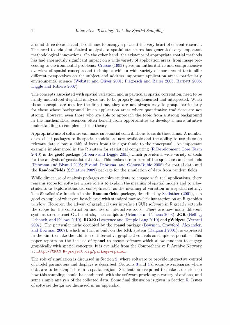
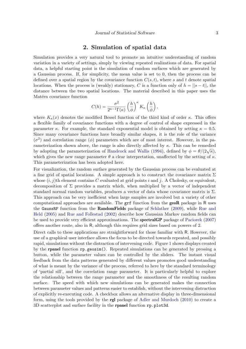
Direct calls to these applications are straightforward for those familiar with R. However, theuse of a graphical user interface allows the focus to be directed towards repeated, and possiblyrapid, simulations without the distraction of intervening code. Figure 1 shows displays createdby the rpanel function rp.geosim(). Repeated simulations can be generated by pressing abutton, while the parameter values can be controlled by the sliders. The instant visualfeedback from the data patterns generated by different values promotes good understandingof what is meant by the variance of the process, referred to here by the standard terminologyof ‘partial sill’, and the correlation range parameter. It is particularly helpful to explorethe relationship between the range parameter and the smoothness of the resulting randomsurface. The speed with which new simulations can be generated makes the connectionbetween parameter values and patterns easier to establish, without the intervening distractionof explicitly re-executing code. A checkbox allows an alternative display in three-dimensionalform, using the tools provided by the rgl package of Adler and Murdoch (2010) to create a3D scatterplot and surface facility in the rpanel function rp.plot3d.

4 Interactive Teaching Tools for Spatial Sampling

Figure 1: Simulations created by the rpanel function rp.geosim(). The top row shows acontour plot, and rgl plot, of a Gaussian process with the Matern covariance function, usingthe parameter values shown in the plot title. The middle row shows the same plots for a secondset of data simulated under the same conditions. The bottom panel shows a contour plot ofdata simulated with a smaller range parameter, together with a plot of the semivariogram.

Journal of Statistical Software 5

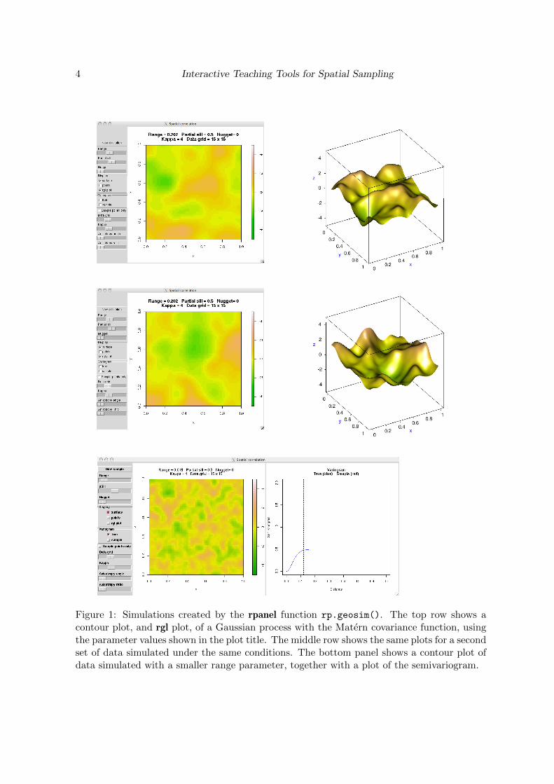
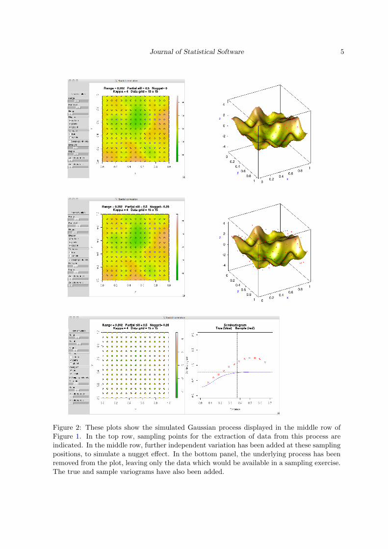
Figure 2: These plots show the simulated Gaussian process displayed in the middle row ofFigure 1. In the top row, sampling points for the extraction of data from this process areindicated. In the middle row, further independent variation has been added at these samplingpositions, to simulate a nugget effect. In the bottom panel, the underlying process has beenremoved from the plot, leaving only the data which would be available in a sampling exercise.The true and sample variograms have also been added.

6 Interactive Teaching Tools for Spatial Sampling

The surfaces shown in Figure 1 represent the entire spatial process. However, it would berare to observe a process in complete form and so it is then helpful to discuss the process ofmeasurement, leading to observed data corresponding to a more limited set of spatial locations.A regular grid of sampling locations is shown in the top two panels of Figure 2. This raisesthe issue of measurement error, or more generally of additional small–scale variation, in theso-called ‘nugget’ effect. A slider is available to control the variance of this additional source ofvariation, represented in the discrepancies between the colors of the points and the underlyingsurface in the contour plot, and more obviously in the separation of points and surface in the3D plot, both shown in the middle panels of Figure 2. Again, repeated simulations andaltered nugget values communicate the meaning of this parameter effectively. It is also usefulto be able to separate simulations which generate new measurement errors on a fixed surfacefrom simulations which generate new values for both. The former type of simulation can beimplemented by checking the ‘Sample points only’ checkbox. This can helpfully illustratea discussion of what it means to take repeated samples of spatial data, and whether theunderlying process or simply the measurement errors will have changed between the repeatvisits.

Finally, it is helpful to suppress the simulated surface and show only the measured values atthe sampling locations. This, of course, is the usual starting point for a spatial analysis andleads, for example, to the construction of a sample semivariogram, as shown in the bottompanel of Figure 2. Repeated simulation at this stage has a further useful role to play indemonstrating the considerable variation which can be exhibited by sample semivariograms.However, more generally, the preceding discussion of the full spatial process as a descriptionof the way the data were generated promotes a deeper understanding of the underlying modeland the meaning of any subsequent fitted parameters.

The rp.geosim function gives control of additional aspects of the simulations, such as thesample size and the value of the κ parameter in the Matern covariance function, as well asangle and ratio parameters for anisotropy. The effects of altering all of these parameters arevery instructive.

3. Mururoa atoll: A spatial sampling scenario

While the analysis of data collected by others in real applications is a very instructive expe-rience, there are some statistical issues which are brought to the fore most effectively whenstudents are confronted with issues of design. The rpanel function rp.mururoa is constructedaround a real sampling context based on the effects of nuclear experiments conducted between1966 and 1996 in the South Pacific, at the atolls of Mururoa and Fangataufa, (IAEA Inter-national Advisory Committee 1998). As part of the assessment of subsequent radiologicalconditions, both terrestrial and aquatic samples were collected and assayed for activities dueto strontium-90, caesium-137, plutonium and tritium. The sampling scenario in rp.mururoa

is based on water sampling by boat for tritium in the Mururoa atoll.

The principle of random sampling is an important one in many application areas and so thisis a natural starting point for Mururoa. However, repeated random selection of samplingpositions, as illustrated in the top two panels of Figure 3, immediately draws attention to thedifficulty that spatial gaps of substantial size may well occur. A more systematic approach, byplacing a regular grid over the region of interest, solves this problem and ensures good spatial

Journal of Statistical Software 7

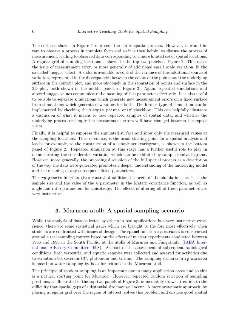
Figure 3: The top two panels show sampling positions for Mururoa Atoll which have beenselected randomly. The left hand middle panel illustrates the use of a regular grid, witha randomly selected starting point. The remaining three panels show line transects withdifferent choices of random and systematic spacing between and within transects.

coverage. The ‘Grid/Transect x-align’ and ‘Grid/Transect y-align’ doublebuttons allowthe grid position to be shifted and raises the issue of how this should be chosen. An element ofrandom sampling can be adopted by selecting the horizontal and vertical location of the gridlines randomly, as illustrated in the left hand middle panel of Figure 3. A further approach isto use line transects, which are well adapted to movement of a boat along a fixed direction andwith the spacing of sampling locations between and/or within transects selected randomly. Asystematic rather than random strategy for both these spacings produces a regular grid whichis no longer oriented in a north-south and east-west direction. Again, the starting positionfor the grid can be selected randomly. All of these options are illustrated in the remainingthree panels of Figure 3. The direction of the transects has been selected to match the broadorientation of the water body within the atoll. This direction could, in principle, itself beselected randomly, although practical considerations in maneouvering the boat may militateagainst that. Finally, for all strategies, the number of sampling points also has to be specified.

The need to make a decision on sampling strategy requires students to think carefully aboutthe consequences for later analysis and this is a very valuable activity. (The reader maywish to consider at this stage which strategy he or she would select.) When a decision has

8 Interactive Teaching Tools for Spatial Sampling

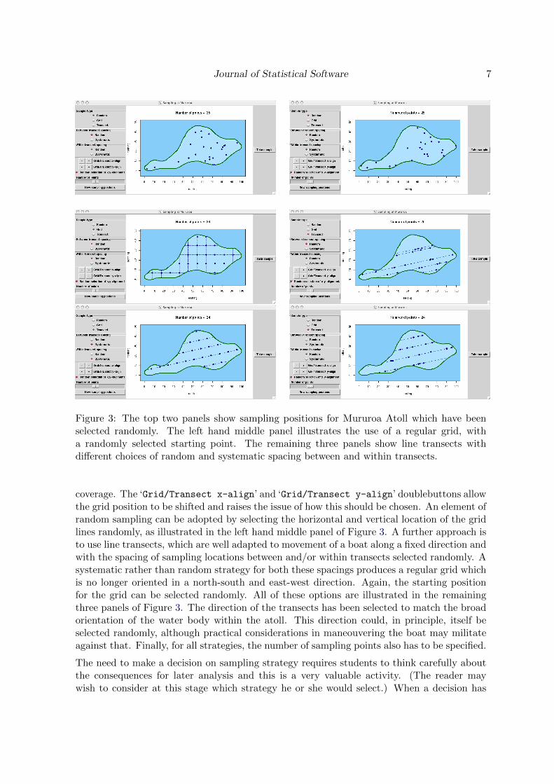
Figure 4: The top panel shows sampled points for Mururoa Atoll, with the observed valuescoded by color. The two middle panels display a predicted surface, with standard errorinformation superimposed as contours, under an assumption of constant trend. The bottompanel shows the true surface (trend plus spatial process) from which the data were simulated.

been made, the ‘Take sample’ button on the right hand size of the panel generates simulateddata, on a scale of kBq/m3 for subsequent analysis. (The structures used to simulate thedata are discussed in Appendix A below.) The controls on the left hand side of the panel arealso disabled, representing the fact that in practice a single decision must be made and its

Journal of Statistical Software 9

consequences lived with.

A new set of controls is now available on the right hand side of the panel. These call geoRfunctions such as variog, variofit, krige.control and krige.conv to perform some simpleanalysis based on kriging, illustrated in Figure 4. The measured values at the samplingpositions, a predicted surface and its standard errors can all be viewed, and choices canbe made on whether a constant, linear or quadratic trend function should be fitted. It isinstructive to view the differences in predicted surfaces which these choices produce, witha quadratic trend prone to more extreme prediction at the edges of the spatial region. Acheckbox is also available to display the structure from which the data were simulated, namelythe trend function plus spatial process. Within the context of a teaching exercise, the abilityto compare predictions with the underlying truth is very helpful.

On some occasions, kriging may run into computational difficulties. The appendix showshow the simulated data may be exported to a file for examination outside the rpanel applica-tion. This allows investigation of whether large spatial gaps, which may occur with randomsampling, are implicated in the computational problem.

4. The sea bed of a firth: Stratified spatial sampling

A second sampling exercise is available in the rpanel function rp.firth. This scenario isbased on the mapping of radioactivity and the calculation of a radionuclide inventory withina water body. (A ‘firth’ is a Scottish term for a long, narrow indentation of the sea coast atthe mouth of a river.) Interest lies in nuclides which, on release into a water body, attach(adsorb) to sediment in a manner which depends on the sediment particle size. Cobalt-60 andcaesium-137 are examples of nuclides which exhibit this behaviour. In this sampling scenario,the map of sediment type is used to define regions of different particle size from which thesediment samples will be collected by grabs from a boat.

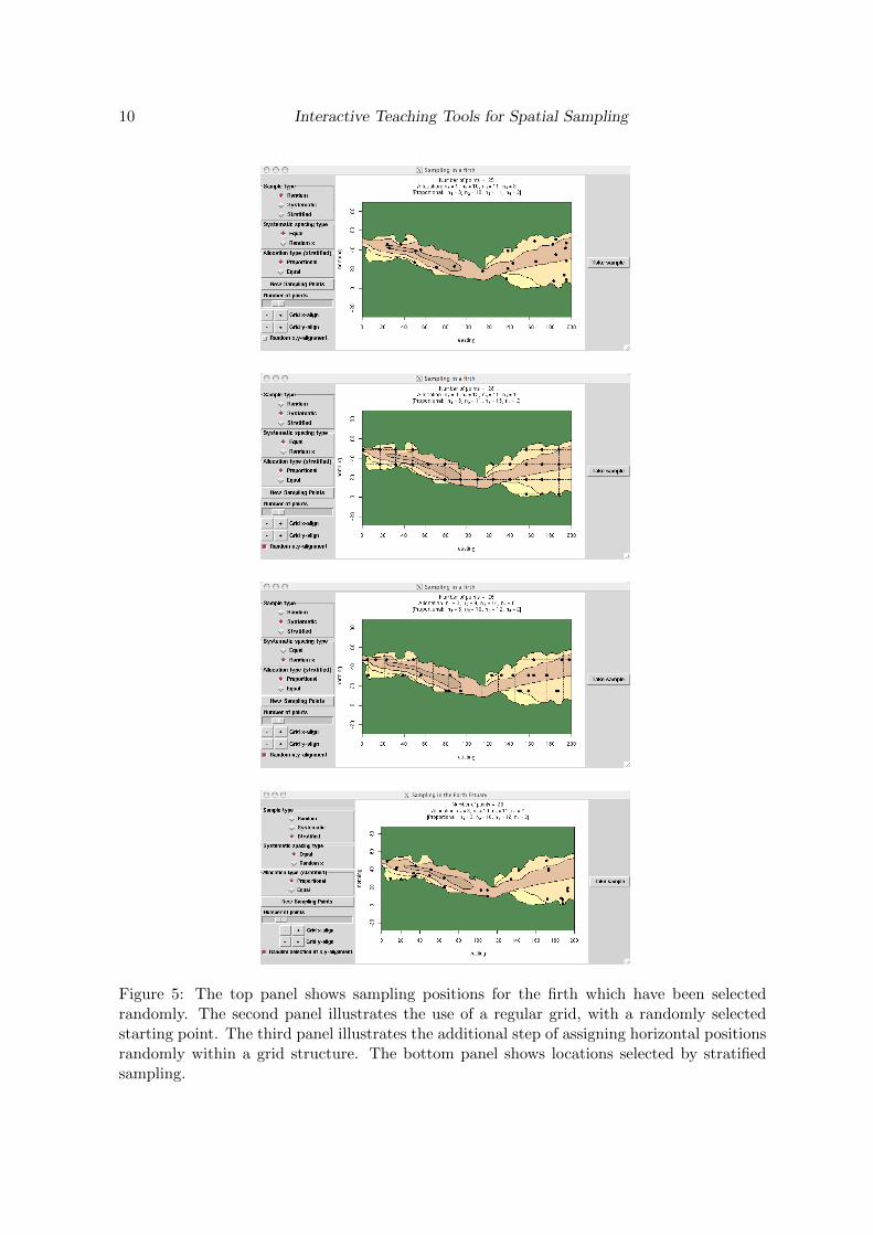
The additional issue to be faced in this scenario is the presence of strata, as the differenttypes of material on the sea bed may affect the mean values of the measurements taken. Oneoption is simply to select sampling positions randomly and hope that this will automaticallycover the strata in a suitable manner. However, as illustrated earlier, this approach suffersfrom the possibility of large spatial gaps. A systematic approach using a regular grid, withrandom selection of the grid starting position, is again available. A further variation is toretain the grid as the basic structure but to allow the horizontal positions of the samplingpoints along the grid lines to be selected randomly. Finally there is an option to focus on thestrata more directly, by carrying out stratified random sampling to ensure that the numberof sampled points in each stratum matches the proportion of the spatial region which eachstratum represents. Even where stratified sampling is not used, the numbers of samplingpositions which fall into each stratum are printed at the top of the panel plot, so that thisaspect of the sampling strategy can be monitored. A number of these different strategies areillustrated in Figure 5.

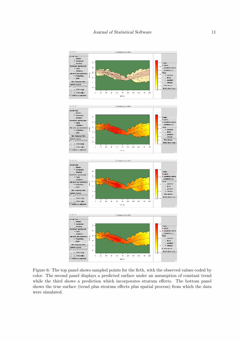
Once a decision has been made, and the ‘Take sample’ button pressed, data are simulatedand presented for analysis. The observed data and a simple spatial prediction are displayedin the top two panels of Figure 6, on a scale of Bq/kg. The additional issue of strata can beincorporated into the prediction process by fitting level shifts, using the likfit function ingeoR. This assumes a model which has a trend function, a single random spatial process plus

10 Interactive Teaching Tools for Spatial Sampling

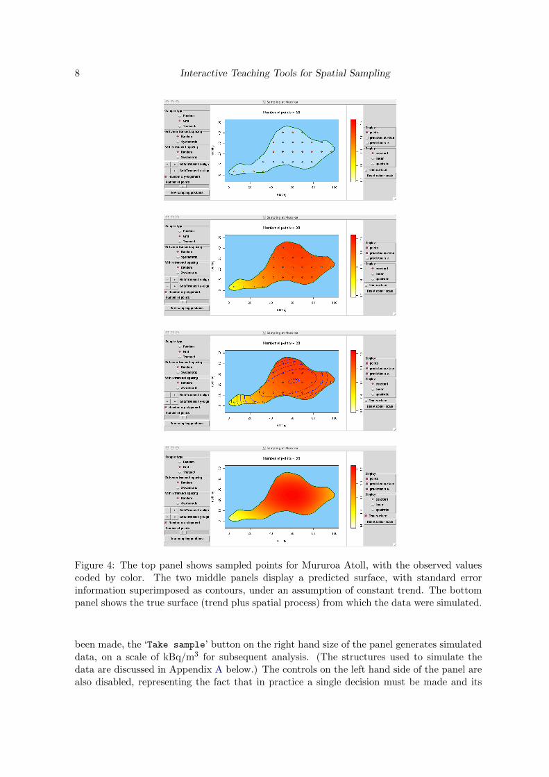
Figure 5: The top panel shows sampling positions for the firth which have been selectedrandomly. The second panel illustrates the use of a regular grid, with a randomly selectedstarting point. The third panel illustrates the additional step of assigning horizontal positionsrandomly within a grid structure. The bottom panel shows locations selected by stratifiedsampling.

Journal of Statistical Software 11

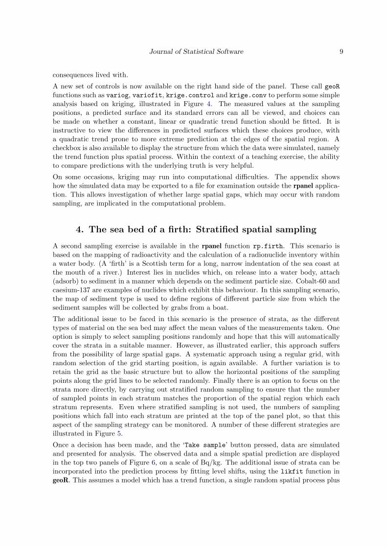
Figure 6: The top panel shows sampled points for the firth, with the observed values coded bycolor. The second panel displays a predicted surface under an assumption of constant trendwhile the third shows a prediction which incorporates stratum effects. The bottom panelshows the true surface (trend plus stratum effects plus spatial process) from which the datawere simulated.

12 Interactive Teaching Tools for Spatial Sampling

a mean shift for each stratum, as well as a nugget effect. This model structure may be beyondthe level of sophistication which is appropriate for students who are meeting spatial data forthe first time. However, even if the technicalities are beyond the grasp of the students, theunderlying concepts can be demonstrated clearly in a graphical manner, through the changesin levels across the strata boundaries in the third panel of Figure 6. Indeed, on this occasionthe data were simulated from a model which did indeed have strata effects, as shown in thebottom panel of Figure 6 where the true data structure is displayed.

5. Discussion

The aim of the tools described in this paper is to enable students and researchers to exploresome of the issues associated with spatial data and models in an interactive manner, to pro-mote intuitive understanding of the concepts involved. In particular, the sampling scenariosprovide contexts in which issues of design have to be considered and this helpfully extendsthe range of activities to which students can be exposed.

Graphical controls for simulation can clearly be implemented to good effect in a much widerrange of application areas. Even within the context of spatial data, it would be straightforwardin principle to apply this to spatial point patterns, for example using the splancs (Rowlingsonand Diggle 2008) or spatstat (Baddeley and Turner 2005) packages.

Teachers may wish to build on the sampling scenarios tools by incorporating other practicalaspects of data collection. For example, information about likely forms of spatial correlationand nugget effects might be added to GUIde sampling strategies. Similarly, decisions on sam-pling strategies have to be taken within the context of budget limits so the costs of samplingcould be given a simple quantification as a fixed overhead plus a component proportional tosample size. The allocation of a fixed budget, or the need to negotiate beyond this, providefurther constraints which students need to consider.

Acknowledgments

The financial support of Ewan Crawford through the Higher Education Academy network forMathematics, Statistics and OR, supported jointly by the university funding councils of theUK, is gratefully acknowledged. The advice of Richard Bowman on hiding the contents offunctions in R is also greatly appreciated.

References

Adler D, Murdoch D (2010). rgl: 3D Visualization Device System (OpenGL). R packageversion 0.91, URL http://CRAN.R-project.org/package=rgl.

Baddeley A, Turner R (2005). “spatstat: An R Package for Analyzing Spatial Point Patterns.”Journal of Statistical Software, 12(6), 1–42. URL http://www.jstatsoft.org/v12/i06/.

Barnett V (2006). Environmental Statistics: Methods and Applications. John Wiley & Sons,London.

Journal of Statistical Software 13

Bivand RS, Pebesma EJ, Gomez-Rubio V (2008). Applied Spatial Data Analysis with R.Springer-Verlag, New York.

Bowman A, Crawford E, Alexander G, Bowman RW (2007). “rpanel: Simple InteractiveControls for R Functions Using the tcltk Package.” Journal of Statistical Software, 17(9),1–18. URL http://www.jstatsoft.org/v17/i09/.

Cressie NAC (1993). Statistics for Spatial Data. John Wiley & Sons, New York.

Dalgaard P (2001). “The R-Tcl/Tk Interface.” In K Hornik, F Leisch (eds.), Proceedings ofthe 2nd International Workshop on Distributed Statistical Computing, March 15–17, 2001,Technische Universitat Wien, Vienna, Austria.

Diggle PJ, Ribiero PJ (2007). Model-Based Geostatistics. Springer-Verlag, New York.

Handcock MS, Wallis JR (1994). “An Approach to Statistical Spatial-Temporal Modeling ofMeterological Fields.” Journal of the American Statistical Association, 89, 368–378.

Helbig M, Urbanek S, Fellows I (2010). JGR - Java GUI for R. R package version 1.7-2,URL http://CRAN.R-project.org/package=JGR.

IAEA International Advisory Committee (1998). The Radiological Situation at the Atolls ofMururoa and Fangataufa: Main Report. International Atomic Energy Agency, Vienna.

Lawrence M, Temple Lang D (2010). “RGtk2: A Graphical User Interface Toolkit for R.”Journal of Statistical Software. Forthcoming.

Paciorek CJ (2007). “Bayesian Smoothing with Gaussian Processes Using Fourier Basis Func-tions in the spectralGP Package.” Journal of Statistical Software, 19(2), 1–38. ISSN1548-7660. URL http://www.jstatsoft.org/v19/i02/.

Pebesma EJ, Bivand RS (2005). “Classes and Methods for Spatial Data in R.” R News, 5(2),9–13. URL http://CRAN.R-project.org/doc/Rnews/.

Piegorsch WW, Bailer AJ (2005). Analyzing Environmental Data. John Wiley & Sons, NewYork.

R Development Core Team (2010). R: A Language and Environment for Statistical Computing.R Foundation for Statistical Computing, Vienna, Austria. ISBN 3-900051-07-0, URL http:

//www.R-project.org/.

Ribeiro PJ, Diggle PJ (2001). “geoR: A Package for Geostatistical Analysis.” R News, 1(2),14–18. URL http://CRAN.R-project.org/doc/Rnews/.

Rowlingson B, Diggle P (2008). splancs: Spatial and Space-Time Point Pattern Analysis.R package version 2.01-27, URL http://CRAN.R-project.org/package=splancs.

Rue H, Follestad T (2002). “GMRFLib: A C-Library for Fast and Exact Simulation of Gaus-sian Markov Random Fields.” Statistics Report 1, Department of Mathematical Sciences,Norwegian University of Science and Technology, Trondheim, Norway.

Rue H, Held L (2005). Gaussian Markov Random Fields. Chapman & Hall/CRC, Florida.

14 Interactive Teaching Tools for Spatial Sampling

Schlather M (2001). “Simulation and Analysis of Random Fields.” R News, 1(2), 18–20. URLhttp://CRAN.R-project.org/doc/Rnews/.

Schlather M (2009). RandomFields: Simulation and Analysis of Random Fields. R packageversion 1.3.41, URL http://CRAN.R-project.org/package=RandomFields.

Tierney L (2005). tkrplot: Simple Mechanism for Placing R Graphics in a Tk Widget.R package version 0.0-19, URL http://CRAN.R-project.org/package=tkrplot.

Urbanek S, Theus M (2003). “iPlots – High Interaction Graphics for R.” In K Hornik,F Leisch, A Zeileis (eds.), Proceedings of the 3rd International Workshop on DistributedStatistical Computing, 2003, Technische Universitat Wien, Vienna, Austria. TechnischeUniversitat Wien, Vienna, Austria. URL http://www.ci.tuwien.ac.at/Conferences/

DSC-2003/Proceedings/.

Verzani J (2007). “An Introduction to gWidgets.” R News, 7(3), 26–33. URL http://CRAN.

R-project.org/doc/Rnews/.

Webster R, Oliver MA (2001). Geostatistics for Environmental Scientists. John Wiley &Sons, Chichester.

Journal of Statistical Software 15

A. Software design

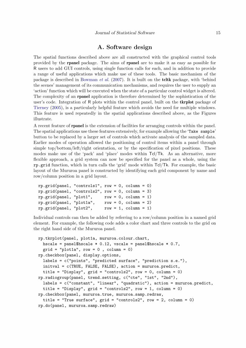
The spatial functions described above are all constructed with the graphical control toolsprovided by the rpanel package. The aims of rpanel are to make it as easy as possible forR users to add GUI controls, using single function calls for each, and in addition to providea range of useful applications which make use of these tools. The basic mechanism of thepackage is described in Bowman et al. (2007). It is built on the tcltk package, with ‘behindthe scenes’ management of its communication mechanisms, and requires the user to supply an‘action’ function which will be executed when the state of a particular control widget is altered.The complexity of an rpanel application is therefore determined by the sophistication of theuser’s code. Integration of R plots within the control panel, built on the tkrplot package ofTierney (2005), is a particularly helpful feature which avoids the need for multiple windows.This feature is used repeatedly in the spatial applications described above, as the Figuresillustrate.

A recent feature of rpanel is the extension of facilities for arranging controls within the panel.The spatial applications use these features extensively, for example allowing the ‘Take sample’button to be replaced by a larger set of controls which activate analysis of the sampled data.Earlier modes of operation allowed the positioning of control items within a panel throughsimple top/bottom/left/right orientation, or by the specification of pixel positions. Thesemodes make use of the ‘pack’ and ‘place’ modes within Tcl/Tk. As an alternative, moreflexible approach, a grid system can now be specified for the panel as a whole, using therp.grid function, which in turn calls the ‘grid’ mode within Tcl/Tk. For example, the basiclayout of the Mururoa panel is constructed by identifying each grid component by name androw/column position in a grid layout.

rp.grid(panel, "controls1", row = 0, column = 0)

rp.grid(panel, "controls2", row = 0, column = 3)

rp.grid(panel, "plot1", row = 0, column = 1)

rp.grid(panel, "plot1a", row = 0, column = 2)

rp.grid(panel, "plot2", row = 1, column = 1)

Individual controls can then be added by referring to a row/column position in a named gridelement. For example, the following code adds a color chart and three controls to the grid onthe right hand side of the Mururoa panel.

rp.tkrplot(panel, plot1a, mururoa.colour.chart,

hscale = panel$hscale * 0.12, vscale = panel$hscale * 0.7,

grid = "plot1a", row = 0 , column = 0)

rp.checkbox(panel, display.options,

labels = c("points", "predicted surface", "prediction s.e."),

initval = c(TRUE, FALSE, FALSE), action = mururoa.predict,

title = "Display", grid = "controls2", row = 0, column = 0)

rp.radiogroup(panel, trend.setting, c("cte", "1st", "2nd"),

labels = c("constant", "linear", "quadratic"), action = mururoa.predict,

title = "Display", grid = "controls2", row = 1, column = 0)

rp.checkbox(panel, mururoa.true, mururoa.samp.redraw,

title = "True surface", grid = "controls2", row = 2, column = 0)

rp.do(panel, mururoa.samp.redraw)

16 Interactive Teaching Tools for Spatial Sampling

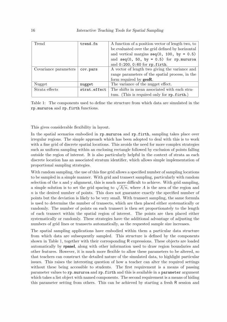
Trend trend.fn A function of a position vector of length two, tobe evaluated over the grid defined by horizontaland vertical margins seq(0, 100, by = 0.5)

and seq(0, 50, by = 0.5) for rp.mururoa

and 0:200, 0:60 for rp.firth.Covariance parameters cov.pars A vector of length two giving the variance and

range parameters of the spatial process, in theform required by geoR.

Nugget nugget The variance of the nugget effect.

Strata effects strat.effect The shifts in mean associated with each stra-tum. (This is required only for rp.firth.)

Table 1: The components used to define the structure from which data are simulated in therp.mururoa and rp.firth functions.

This gives considerable flexibility in layout.

In the spatial scenarios embodied in rp.mururoa and rp.firth, sampling takes place overirregular regions. The simple approach which has been adopted to deal with this is to workwith a fine grid of discrete spatial locations. This avoids the need for more complex strategiessuch as uniform sampling within an enclosing rectangle followed by exclusion of points fallingoutside the region of interest. It is also particularly helpful in the context of strata as eachdiscrete location has an associated stratum identifier, which allows simple implementation ofproportional sampling strategies.

With random sampling, the use of this fine grid allows a specified number of sampling locationsto be sampled in a simple manner. With grid and transect sampling, particularly with randomselection of the x and y alignment, this is much more difficult to achieve. With grid sampling,a simple solution is to set the grid spacing to

√A/n, where A is the area of the region and

n is the desired number of points. This does not guarantee exactly the specified number ofpoints but the deviation is likely to be very small. With transect sampling, the same formulais used to determine the number of transects, which are then placed either systematically orrandomly. The number of points on each transect is then set proportionately to the lengthof each transect within the spatial region of interest. The points are then placed eithersystematically or randomly. These strategies have the additional advantage of adjusting thenumbers of grid lines or transects automatically, as the requested sample size increases.

The spatial sampling applications have embodied within them a particular data structurefrom which data are subsequently sampled. This structure is defined by the componentsshown in Table 1, together with their corresponding R expressions. These objects are loadedautomatically by rpanel, along with other information used to draw region boundaries andother features. However, it is much more flexible to allow these parameters to be altered, sothat teachers can construct the detailed nature of the simulated data, to highlight particularissues. This raises the interesting question of how a teacher can alter the required settingswithout these being accessible to students. The first requirement is a means of passingparameter values to rp.mururoa and rp.firth and this is available in a parameter argumentwhich takes a list object with named components. The second requirement is a means of hidingthis parameter setting from others. This can be achieved by starting a fresh R session and

Journal of Statistical Software 17

executing the following code which, in this case, simply sets the stratum effects of rp.firthto zero.

spatial.samp <- function(arg) rp.firth(parameters = arg)

hideargument <- function(f, arg) function() f(arg)

spatial.sampling <- hideargument(spatial.samp,

list(strat.effect = rep(0, 4)))

rm(hideargument)

The workspace should then be saved in a file. Students can then load this workspace file andlaunch the customized software simply by making the function call spatial.sampling().The required information is lifted from the appropriate environment without being directlyaccessible by students.

It is also possible to write the sampled data to a file for more extensive analysis by othermeans. This is achieved simply by specifying a filename in the file argument of rp.mururoaand rp.firth.

Affiliation:

Adrian W. BowmanDepartment of StatisticsThe University of GlasgowGlasgow G12 8WW, United KingdomE-mail: adrian@stats.gla.ac.ukURL: http://www.stats.gla.ac.uk/~adrian/

Journal of Statistical Software http://www.jstatsoft.org/

published by the American Statistical Association http://www.amstat.org/

Volume 36, Issue 13 Submitted: 2008-12-15October 2010 Accepted: 2010-02-03