Embed Size (px)
Citation preview

NUREG/CR-4928
0�� -- wwwwm�h
Degradation of Nuclear PlantTemperature Sensors
Prepared by H. M. Hashemian, K. M. Peterson,R. L. Anderson, K. E. Holbert
T. W. Kerlin,
Analysis and Measurement Services Corporation
Prepared forU.S. Nuclear RegulatoryCommission

NOTICE
This report was prepared as an account of work sponsored by an agency of the.United StatesGovernment. Neither the United States Government nor any agency thereof, or any of theiremployees, makes any warranty, expressed or implied, or assumes any legal liability of re-sponsibility for any third party's use, or the results of such use, of any information, apparatus.product or process disclosed in this report, or represents that its use by such third party wouldnot infringe privately owned rights.
NOTICE
Availability of Reference Materials Cited in NRC Publications
Most documents cited in NRC publications will be available from one of the following sources:
1. The NRC Public Document Room, 1717 H Street, N.W.Washington, DC 20555
2. The Superintendent of Documents, U.S. Government Printing Office, Post Office Box 37082,Washington, DC 20013-7082
3. The National Technical Information Service, Springfield, VA 22161
Although the listing that follows represents the majority of documents cited in NRC publicatic i,it is not intended to be exhaustive.
Referenced documents available for inspection and copying for a fee from the NRC Public Docu-me-,t Room include NRC correspondence and internal NRC memoranda; NRC Office of Ins. ectionand Enforcement bulletins, circulars, information notices, inspection and investigation notices;Licensee Event Reports; vendor reports and correspondence; Commission papers; and applicant andlicensee documents and correspondence.
The following documents in the NUREG series are available for purchase from the GPO SalesProgram: formal NRC staff and contractor reports, NRC-sponsored conference proceedings, andNRC booklets and brochures. Also available are Regulatory Guides, NRC regulations in the Code ofFederal Regulations, and Nuclear Regulatory Commission Issuances.
Documents available from the National Technical information Service include NUREG seriesreports and technical reports prepared by other federal agencies and reports prepared by the AtomicEnergy Commission, forerunner agency to the Nuclear Regulatory Commission.
Documents available from public and special technical libraries include all open literature items,such as books, journal and periodical articles, and transactions. Federal Register notices, federal andstate legislation, and congressional reports can usually be obtained from these libraries.
Documents such as theses, dissertations, foreign reports and translations, and non-NRC conferenceproceedings are available for purchase from the organization sponsoring the publication cited.
Single copies of NRC draft reports are available free, to the extent of supply, upon writtenrequest to the Division of Information Support Services, Distribution Section, U.S. NuclearRegulatory Commission, Washington, DC 20555.
Copies of industry codes and standards used in a substantive manner in the NRC regulatory processare maintained at the NRC Library, 7920 Norfolk Avenue, Bethesda, Maryland, and are availablethere for reference use by the public. Codes and standards are usually copyrighted and may bepurchased from the originating organization or, if they are American National Standards, from theAmerican National Standards Institute, 1430 Broadway, New York, NY 10018.

NUREG/CR-4928
Degradation of Nuclear PlantTemperature Sensors
Manuscript Completed: May 1987Date Published: June 1987
Prepared byH. M. Hashemian, K. M. Petersen, T. W. Kerlin,R. L. Anderson, K. E. Holbert
Analysis and Measurement Services Corporation9111 Cross Park Drive, NWKnoxville, TN 37923-4599
Prepared forDivision of EngineeringOffice of Nuclear Regulatory ResearchU.S. Nuclear Regulatory CommissionWashington, DC 20555NRC FIN D1712
ABSTRACT
A program was established and initial tests were performed to evaluatelong term performance of resistance temperature detectors (RTDs) of the typeused in U.S. nuclear power plants. The effort addressed the effect of agingon RTD calibration accuracy and response time. This Phase I effort includedexposure of thirteen nuclear safety system grade RTD elements to simulated LWRtemperatures. Full calibrations were performed initially and monthly, sensorswere monitored and cross checked continuously during exposure, and responsetime tests were performed before and after exposure. Short term calibrationdrifts of as much as 1.81F (1-C) were observed. Response times wereessentially unaffected by this testing.
This program shows that there is a sound reason for concern about theaccuracy of temperature measurements in nuclear power plants. These limitedtests should be expanded in a Phase II program to involve more sensors andlonger exposures to simulated LWR conditions in order to obtain statisticallysignificant data. This data is needed to establish meaningful testing orreplacement intervals for safety system RTDs. An important corollary benefitfrom this expanded program will be a better definition of achievableaccuracies in RTD calibration.
This report concludes a six-month Phase I project performed for theNuclear Regulatory Commission under the SEIR program.
iii

TALE OF cawS
Section
1* INTRODUCTION . . . . . . . . . . . . * . * ** 4 4 * 4 * * 4 * .
1.1 Project Objectives . . . . . . . . . . . . .1.2 Project Importance . . . . . . . . . . . . . .1.3 Work Completed in this Project . . . . . . .
2. STATIC ACCURACY AND DYNAMIC RESPONSE.
2.1 Static Accuracy . . . . . . . . . . . . .2.2 Dynamic Response . . . . . . . . . . . . . .
3. RTD PERFORMANCE REQUIREMENTS IN NUCLEAR POWER PLANTS
4. LABORATORY TESTING METHODS . . . . . . . . . a. . ..
4.1 Static Performance Testing. . . . . . . .4.2 Dynamic Performance Testing . . . . . . . . . .
5. LABORATORY TEST RESULTS . . . . . . . . . . . . .
5.1 Description of the Sensors . . . . . . .5.2 Static Tests . o . ... ... .. . . ..5.3 Dynamic Tests . . . . . . . . . . . . . . . .
6. IN-SITU TESTING METHODS . . . . . . . . . . . . . .
6.1 Calibration Checking . . . . . . . . . . .6.2 Response Time Testing . . . . . . . . . . . . .
4 . . 4 4 �
4-. . 4 * �
. . . . . . .
* . . . . . 4
. . . . . . ..
. . . . . 4 .
. . . 4 * * �
4 . . . . . 4
PaRe
1
112
3
35
7
9
912
15
151528
30
3031* a * * * a * .
7. CONCLUSIONS AND RECOMMENDATIONS 33* . a. . . . a * a * * * . *
APPENDICES -
Appendix A: Performance of Platinum Resistance Thermometers inNuclear Power Plants
v

LIST OF FIGURES
FiRure
2.1
2.2
-4.1
4.2
Description
Simplified schematic of a typical RTD . . . . . . . . . . .
Typical response of an RTD to a step change in temperature
RTD calibration system . . . . . . . .
RTD drift testing system ............... .'
PaRe
4
6
10
11
4.3
4.4
5.1
5.2
5.3
5.4
5.5
5.6
5.7
5.8
5.9
5.10
6.1
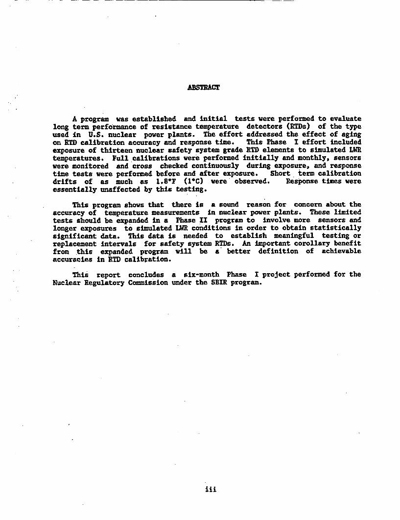
RTD calibration shift as a function of temperature.
RTD calibration shift as a function of temperature-
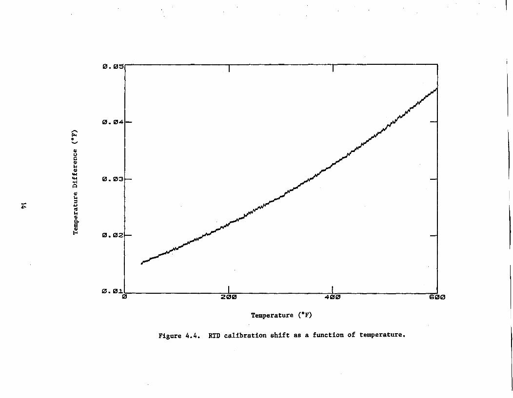
Time history for a stable RTD . . . . . . . . . .
Time history for a drifting RTD . . . . . . . . .
Average temperature in the furnace ..... . . .
Temperature drift in -the RTDs after one month . . . . .
Temperature drift in the RTDs during second month . . .
Temperature drift in the RTDs during third month
Temperature drift in RTDs for three months of thermal al
Changes in alpha for the RTDs . . . . . . . . . .
Changes in delta for the RTDs . . . . . . . . . .
Changes in ice-point resistance for the RTDs . .
Sensor input-output processing of fluctuating signals'
. . . 0 0
::!* 6
0 a
.0 0 . .
. 0 0 0
. 0 . . a
. . * * .
Lging . . .
.. * . 0 0
13
14
17
18
19
20
21
22
24
25
26
27
32
. . . . 0
vi

1. -aRODu
1.1 Proiect Objectives
The objectives of this Phase I research effort were:
1. Identify and evaluate static and dynamic performancerequirements on resistance temperature detectors (RTDs) ofthe type used for safety related temperature measurements inU.S. nuclear power plants.
2. Develop a test program to. evaluate degradation incalibration and response time of RTDs as they age. in anuclear power plant.
3. Initiate laboratory testing according to the programdeveloped under objective 2.
4. Evaluate performance limits and testing intervals for RTDrequalification or replacement.
5. Evaluate available methods for testing the performance ofRTDs as installed in an operating plant (in-situ testing).
1.2 Project Importance
RTDs are essential components of many LWR safety systems. Theirindications must be accurate and timely in order for the safety system tooperate properly. This can be achieved only by assuring initial, as-installedaccuracy and response times and by determining possible drift rates in both ofthese quantities. The drift rate information is essential for establishingproper recalibration or replacement schedules.
Performance requirements on measurement accuracy and response time ofnuclear plant RTDs both approach technically achievable limits. Therefore, itis essential to optimize sensor design, selection and use and to determinereliable information on achievable performance limits.
I

1.3 Work Completed in this Project
The objectives stated in the Phase I proposal were met in this project.Furthermore, the laboratory testing to evaluate sensor degradation progressedsignificantly further than anticipated. The specific accomplishments are:
1. Identification of performance requirements. Response timeand accuracy requirements were identified for eight nuclearpower plants. The results are shown in Section 3 of thisreport.
2. Test Program Development. A test program was developed andfacilities were assembled for assessing changes in sensoraccuracy when exposed to simulated thermal environments innuclear power plants. This program included sensorcalibration, thermal aging in a simulated reactorenvironment, drift monitoring as sensors aged, periodicinsulation resistance measurements, and response timetesting before and after aging.
3. Initial Laboratory Testing. Thirteen typical nuclear gradeRTD elements were exposed to 637P7 (3361C) air in a furnacefor three months. Readings were made on each sensor everyfive minutes. Each sensor was removed monthly for a fullcalibration. Response time testing was performed initiallyand after the three-month aging period. Test results arepresented in Section 5.
4. Performance Limits. The three month exposure of thirteensensors to drift testing at typical LWR conditions providesa small initial entry to the data base needed for meaningfulstatistical assessment of performance. Results arepresented in Section 5.
5. In-Situ Testing Methods. Possible methods for in-situperformance testing of RTDs were reviewed. Theinvestigation is reported in Section 6.
6. Performance of Platinum Resistance Thermometers in NuclearPower Plants. To provide a vehicle for exchanginginformation among members of the AMS research team and forcommunicating with other interested parties, a review paperwas prepared. It is included as Appendix A of this report.
2

2. STATIC ACCURACY AND DYNAMIC RESPONSE
2.1 Static Accuracy
A nuclear plant RTD is generally a stainless steel sheathed sensor asshown schematically in Figure 2.1. In some plants the sensors are installedin thermowells and in others they are inserted into primary loop water flowingthrough a by-pass manifold. The resistance element is platinum doped with atrace of rhodium so as to give a temperature dependent resistivity which canbe achieved reproducibly and economically. The platinum may be a wire or afilm mounted on an insulating support structure. Special effort is spent toachieve ruggedness yet adequate freedom of motion of the platinum relative tothe support structure. This freedom of motion is to avoid strain effectscaused by differential thermal expansion which could interfere withtemperature measurements.
The resistance at a selected, reference temperature is adjusted byselecting the cross sectional area and length of the platinum. Ice pointresistances are used as references and typical values for nuclear plant RTDsare 100 ohms and 200 ohms. The temperature (T) vs. resistance (R) relation isusually represented as a second order polynomial. One form is
R = a + bT + cT2 (2.1)
The sensitivity is approximately 0.385Z resistance/"C.
Sensors are built in three wire and four wire configurations. Thesepermit compensation for the effects of lead wire resistance (See Appendix A).
Calibration of an RTD involves measuring the resistance at three or moreknown temperatures. The R vs T values are then fit to an equation of the formof Equation 2.1. The equation with the fitted coefficients is then used togenerate calibration tables (R vs T at any temperature of interest). Thecalibration data are then used to tune the RTD transmitters which converts theresistance to an equivalent voltage or current. The accuracy of the indicatedtemperature depends on the accuracy of the RTD calibration and the RTD driftrate which are addressed in this project.
3

- -
metal sheath
Lead wIies
Ft I ler(powder or cement)
- , - Mandrel(with platinum element)
Figure 2.1. Simplified schematic of atypical RTD.
4

2.2 Dynamic Response
Because of heat diffusion effects, temperature sensors always lag behindchanging process temperatures. A typical RTD response to a step change intemperature is shown in Figure 2.2. An index used to characterize sensorresponse is the time constant, defined as the time required for the responseto reach 63.2 percent of the total change following a step in monitoredtemperature.
Sensor time constants increase with increased heat capacity of sensorconstituents and with increased thermal resistance between the sensing elementand the monitored fluid.
Responses of sensors used in thermowells are strongly affected by the fitbetween the sensor and the thermowell because of the large thermal resistancecaused by small gaps in the heat transfer path.
Sensor time constants for RTDs in nuclear power plants generally rangefrom 0.1 sec to over 10 sec. The fast sensors are special, direct immersionsensors which are designed to have a very low heat capacity and a very lowthermal resistance. Typical time constants for sensors in thermowells are 5sec to 10 sec. Time constants as large as 40 sec have been measured in caseswhere the sensor/thermowell fit was poor.
5

-
T2
I-i!
'aC.
63. Dz( T2-TI)
TIME
Figure 2. 2. Typical response of an RTD to a step changein temperature.
6

3. KTD PERFORMANCE UIREENTS IN NUCLEAR POWER PLANTS
Eight utilities were contacted to determine accuracy and response timerequirements for safety system RTDs. The results are shown in Table 3.1.This limited survey indicated accuracy requirements between 0.02'F (O.O1C)and 2.5'F (1.4-C) and time constant requirements between 4 sec and 15 sec.This survey was very informal. Plant instrumentation technicians or engineersprovided their best knowledge of sensor requirements from purchasingspecifications or technical specifications. The information was obtained intelephone interviews. The lesson from this survey is the order of magnitudeof performance requirements and the wide range of requirements at differentplants.
7

TABIL 3.1
Typical MID Performance Requdrmnts in Various Operating Nuclear Power Plants
Sensor Type
In Thermowell
In Thermowell
In Thermowell
Direct Immersion
Direct Immersion
In Thermowell
In Thermowell
In Thermowell
Accuracy & Drift Requirements
±2.56F total channel accuracy(including drift)
0.31-F RTD calibration accuracy 0 to 750'F1.091F (total channel accuracy including 22month drift)
±1.50F for sensor cross calibration
±0.5'F calibration accuracy±1.2'F for sensor cross calibration±0.70F drift/18 months
±0.2-F calibration accuracy±0.50 drift for life of plant
±0.4% (from 520-620'Y) calibration accuracy(40 year repeatability:0.05% of initial calibration at 321F)
1% of the reading
±0.020F calibration accuracyRepeatability t0.20F
Response TimeRequirement
13 sec (hot leg)8 sec (cold leg)
6 sac
8 sec
4 sec for RTD, rackand breaker (Rack &Breaker 0.1 sec each)
4 sec for total,channel
4 sec
15 sec
4 sec
/

4. LBOR&TOURY TESTING KETHODS
4.1 Static Performance TestinR
The static performance testing program required automation of calibrationcapability and construction of test facilities for providing simulated LWRconditions for drift testing.
The calibration approach developed is a balance between accuracy, easeand speed of calibration, and cost. The system includes:
1. A Hewlett-Packard Model 3457A precision digital multimeterfor measuring RTD resistance to be converted to equivalenttemperature.
2. An ice bath and an oil bath with agitator and temperaturecontroller. The sensors were installed in a copper block inthe oil bath to improve temperature stability.
3. Precision reference RTDs for measuring the bath temperature.
4. A rotary switch box for switching between reference RTDs andthe RTDs under calibration.
The calibration uses the comparison method which involves measurement ofthe bath temperature (with a precision reference RTD) and the resistance ofthe RTD being calibrated. The sensor being calibrated was installed in thecopper block adjacent to the precision RTD. After the two sensors reachedthermal equilibrium, resistance measurements were made on both sensors. Thereference sensor's calibration was used to obtain the bath temperature. Apicture of the calibration set up is given in Figure 4.1.
An ATS Model 3210 three-zone tube furnace was purchased and adapted toprovide a simulated LWR thermal environment for aging tests. The furnace wasdrilled to hold 15 sensors. A temperature controller was installed to controlthe furnace temperature. The temperature aging of the RTDs was done at about637OF (336*C).
The sensors were all connected, to a Hewlett-Packard Model 3488Aswitch/control unit. The set-up is shown in Figure 4.2. Each sensor wasmonitored every five minutes to detect sudden failures and to collect data tocheck for any gross drift during the aging process. The measurements were fed
.9

0
Figure 4.1. RTD calibration system.

xts.� ��j4s
* '**#
Figure 4.2. RTD drift testing system.

to an IBM computer where the data are stored and processed. The processinginvolved calculating average readings from all sensors and deviations from theaverage value. Software was developed to permit user friendly operation ofthe data collection, data processing and hard copy results preparation.
Computer software previously developed at AMS was used to fit thecalibration data to the Callendar equation. The Callendar equation isdiscussed in Appendix A and is repeated below:
R rT TK = 1 + C[T- (lo )(EO-O
where
R(T) = PRT resistance at temperature, T
RO, a, 6 - fitting coefficients
This form of the fitting equation is used for temperatures above 32'F (0C).After the fit is complete, the computer program may be used to generate acalibration table (R vs T).
Sensors were removed from the furnace on a monthly schedule andcalibrations were performed. The monthly calibration results for each RTDwere compared to determine if temperature aging had caused calibrationchanges. A computer program was written to perform the comparison and plotthe difference at all temperatures within the calibration range. Figures 4.3and 4.4 show a sample of two RTD comparison plots obtained in the program.
4.2 Dynamic Performance TestinR
The dynamic performance testing was accomplished using the plunge testmethod. The steps are as follows:
1. Insert the sensor into a stream of heated air until itreaches thermal equilibrium.
2. Rapidly insert the sensor into a stream of water flowing atthree feet per second.
3. Monitor the sensor signal on a strip chart recorder anddetermine the time constant by identifying the time requiredto reach 63.2 percent of the total change.
12

0.
0.1 _
@14
5.1
.iI0. 0-
E.4
-0. 1|
0 200 400 600
Temperature (OF)
Figure 4.3. RTD calibration shift as a function of temperature.
0. 05
0. 04
O fP4
4t 0.03_
E- 0. 02-_'.4
0. 0.2.-0 200 400
Temperature (CF)
Figure 4.4. RTD calibration shift as a function of temperature.

S. L&BORATORY TEST RESULTS
5.1 Description of the Sensors
Ten nuclear grade RTDs including three dual element sensors were testedin this study. A listing of these RTDs representing a total of thirteenelements is given in Table 5.1. A tag number was assigned to each RTD foridentification during this project. These RTDs include at least one from eachof the manufacturers of nuclear qualified RTDs. They were selected from thoseavailable at AMS and a few which were provided by interested utilities andmanufacturers. This included both new and used RTDs., As such, they were anon-ideal set of test sensors because their past histories are unknown.Nevertheless, they are suitable for the testing program initiation implementedin this work.
5.2 Static Tests
The tests provided two types of data: time histories of deviations frommeasured average temperatures for each sensor and changes in sensorcalibration at each monthly test.
Figure 5.1 shows the time history for one of the RTDs while in thefurnace for approximately one month. It was obtained by subtracting the RTDindication from the average furnace temperature. The mean of the differencehas been removed to account for spatial temperature variations in the furnace.The time history indicates that the RTD closely followed the average furnacetemperature (within ±O.1F) and was therefore stable during the period.Figure 5.2 shows a time history plot with indication of drift during the sameperiod. The average furnace temperature for this period is shown in Figure5.3. Time history plots were generated for all the RTDs in this program andthe results were compared with those of the monthly calibrations. It wasconcluded that the time history plots are useful for tracking grosscalibration shifts but accurate measurements require the full calibration aswas performed monthly in this program.
Results of monthly calibration tests are shown in Figures 5.4 through5.6. These figures show deviations from the initial calibration attemperatures of 321F, 2001F, 4001F and 600'F. The horizontal axis gives theRTD tag number and the vertical axis gives the temperature drift at fourdifferent temperatures. A precision reference RTD was also included in theprogram and was calibrated every month along with the other RTDs to provide ameasure of our calibration repeatability. The results for this RTD is plottedas CTRL. This RTD was not exposed to temperature aging in the furnace.
The data plotted in Figure 5.6 through 5.4 were obtained by the followingprocedure:
15

TAM-E 5.1
Listing of RTDs Tested
Item Taxi Description
1 01 Single Element Direct Immersion2 03 Single Element Well Type3 04A Dual Element Well Type. Element 14 04B Dual Element Well Type. Element 25 5A Dual Element Well Type. Element 16 5B Dual Element Well Type. Element 27 6A Dual Element Well Type. Element 18 6B Dual Element Well Type. Element 29 07 Single Element Well Type10 08 Single Element Well Type11 09A Dual Element Well Type. Element 112 09B Dual Element Well Type. Element 213 10 Single Element, Direct Immersion
16
1.00 -
0.90
0.80 -
0.70
0.60 -
0.500.40-
* 0.30-
h 0.20* 0.10
0.00-
g -0.10
-0.20
d -0.30
* -0.40
-0.50
-0.60-0.70
-0.80
-1.00
0 100 200 300 400 500
Time (Hours)
Figure 5.1. Time history for a stable RTD.

1.00
0.90
0.600
0.70 -
0.60
0.500.40
0.30
0.20
*M 0.10
0.00-
_ a -0.10000
w ° -0.20
g -0.30
-0.40
-0.50-
-0.60-0.70
-0.80
-0.90
-1.00 -
0 100 200 300 400 500
Time (Hours)
Figure 5.2. Time history for a drifting RTD.

Month 3640.0
'-4
'4
'4
V
C0
639.0 -
638.0 -
637.0 -
636.0 -
635.0 �1
0 100 200 300 400
Time (Hours)
Average temperature in the furnace.
500
Figure 5.3.

Month I
a00
'4to6
0Q
%a14d
'4Cp.a
pi
3
2.5
2
1.5
0.5
0
-0.5
-1
-1.5
-2
NJ'.
01 03 04A 04B 05A 05B 06A 06B 07 08 09A 09B 10 CTRL
r 1 32 FRTD Element Taj Number
200 F V3 400 F 600 F
Figure 5.4. Temperature drift in the RTDs after one-month.

Month 23 -
0054
054%O
54
14
54Sp.
2 -
1 -
~ _ T .. PL - -. I L9 F i0
-1
M A , N =CZ= ==mmEld & ENd0000I
6
-2 I I I I I I I I01 03 04A 04B 05A 05B 06A 06B
I I I I I I.07 08 09A 09B 10 CTRL
V/l 32 FRTD Element Tat Number
= 200 F M 400 F Mi 600 F
Figure 5.5. Temperature drift in the RTDe during second month.

Month 33
F4
0
'40'4
*.W
'40
S4
e
1
K).0
-1
-2
01 03 04A 04B 05A 05B 06A 06B 07 08 09A 09B 10 CTRL
P71 32 FRTD Element T Number
200 F f 400 P B00 F
Figure 5.6. Temperature drift in the RTDs during third month.

1. calibrate each sensor at the ice point and three othertemperatures between the ice point and about 6001F (315eC)
2. place the sensor in the furnace at 6371F for approximatelyone month
3. remove sensor from furnace and calibrate per Step 1 above
4. fit R vs T data to the Callendar equation
5. use the Callendar equation with fitted coefficients toevaluate the resistance of 32°F, 200'F, 4001F and 6001F
6. calculate the difference between the temperature obtainedfrom the original calibration and the current calibration.
Figure 5.4 shows the changes which occurred in the indication of each RTDafter one month of thermal aging. For example, RTD number 03 showed verylittle change at 32-F, but it read between -0.5 to -1'F low at 2001F and 4001Fwhile at 6001F it only had about +O.lF error. Element number 04A is the onethat showed the largest error at all four temperatures (between 1.5'F to 2.5SFhigh). Element number 06A was the most stable RTD with very little change atall temperatures. Note that the changes in the indication of the referencesensor (CTRL) is very small indicating good repeatability for the calibrationsystem. RTD number 01 was not in the program during the first month.
Figures 5.5 and 5.6 show the changes that occurred during the second andthird months respectively. The changes represent one-month drift from thebeginning to the end of the second month (Figure 5.5) and from beginning tothe end of the third month (Figure. 5.6). It is apparent that the calibrationof all RTDs stabilized after the first month. The changes are much smallerduring the second month and even smaller during the third month. The combinedchanges are shown in Figure 5.7 indicating that after three months of thermalaging the RTDs drifted by up to about 1IF except for RTD number 04B and 07whose errors were in the 1OF to 21F range.
The calibration data were also used to obtain the deviations in a, 6 andRO (the parameters of Callendar equation used for fitting the data). The dataare plotted in Figures 5.8. 5.9 and 5.10. Each plot provide the changesduring first, second, and third month for all the RTDs tested and the CTRLRTD. These plots support our earlier conclusion that most of the shift in thecalibration of the RTDs occurred in the first month and that the RTDsstabilized in the second and third month.
The insulation resistance (element to sheath) of each RTD was alsomeasured each month after the RTD was removed from the furnace. These weremeasured at ambient temperature with 100 VDC applied across the sensor sheathand one of the RTD leads. The values were generally above the acceptablevalue of 100 megohms and remained so during the program.
23

Full Period3
UDW
0Sto
to
S
'4d
%O
a
'4
'4S
PinS
2
0NJ.P.
-201 03 04A 04B 05A 05B 06A 06B 07
RTD Element t NumberPJ 32 F I= 200 F M 400 F
08 09A 09B 10
M 600 F
CTRL
Figure 5.7. Temperature drift in RTDs for three months of thermal aging.

2
I
A^
do 10
g o
, _tU
C)
0
-1
-2I IPI
-3
-4 I I I
01 03 04A
ZZ/ Month 1
I I I I I I04B 05A 05B 06A 06B 07
RTD Element Tag NumbersF,9 Month 2
I I I I08 09A 09B 10
I-CTRL
go Month 3
Figure 5.8. Changes in alpha for the RTDs.

0.1
0.0
Id
.P4
-0.1
-0.2
-0.3
N0%
c
.a
U
-0.4
-0.5
01 03 04A 04B OA 05B 06A 06B 07 08 09A 09B 10 CTRL
0Z1 Month IRTD Element Tag Numbers
j;9 Month 2 M .Month 3
Figure 5.9. Changes in delta for the RTDs.

0'S
q4
Ais
1.1
1.0
0.9
0.8
0.7
0.6
0.5
0.4
0.3
0.2
0.1
0.0
-0.1
-0.2
-0.3
-0.4
-0.5
I lEE
n r, - rq rtf-I
H.l, , d , - -_
I I I I I I01 03 04A 04B 05A 05B
I I06A 06B 07
I I I I08 09A 09B 10 CTRL
IZZ Month IRTD Element Tag Numbers
=~ Month 2 Month 3
Figure 5.10. Changes in Ice-point resistance for the RTDs.

5.3 Dynamic Tests
Plunge tests were performed onto simulated LWR conditions and againresults are summarized in Table 5.2.04 and 09 was tested and that thethermowell.
all sensors before the start of exposureafter a three month exposure. The
Note that only one element of RTD numberwell-type RTDs were tested without a
These results showed that the exposure to simulated LWR conditions hadlittle or no effect on time response. This is consistent with extensive AMSexperience in measuring the time response of sensors in operating nuclearpower plants. This experience shows that although time response problems arecommon, they are predominantly the result of imperfect fits between sensorsand thermowells for well-type RTDs.
28

TAMBLE 5.2
Response Time Test Results
TimeInitially
Constant (see)After 3 Months
01030405A05B06A06B07080910
2.11.42.11.21.41.91.81.03.52.70.9
2.11.42.01.11.31.71 .61.13.22.50.9
29

-
6. IN-SITU TESTING HMMTRDS
This section reviews the current status of in-situ testing forcalibration checking and response time checking.
6.1 Calibration Checking
Research has been in progress for several years on the use ofJohnson Noise techniques to perform a one point calibration check while theRTD remains installed in a normally-operating plant. The principle is thattemperature dependent voltage and current fluctuations occur in any resistorbecause of statistical variations in the spatial free electron population. Ithas been shown that temperature can be determined by monitoring thesestatistical fluctuations. The measurement has great appeal because it doesnot depend on the material properties of the resistor. It requiresintegration over a period of time to process the signals and obtain anestimate of the temperature. Longer processing times give better accuracy.The physics underlying this measurement technique has been known for almostfifty years, but practical implementation required two new developments:amplifiers capable of handling very low level signals (nanovolts and nanoamps)and a means to handle the filtering effect of cables between the sensor andthe amplifier. Advances in the technology (mainly by Blalock, Shepard andRoberts at Oak Ridge National Laboratory and Brixy of West Germany) havefurnished the instrumentation and several methods to deal with the cableeffects. Three approaches are possible for overcoming the cable problem:
- Perform the measurement at the head of the sensor. Thiseliminates the cable, but results in radiation doses for theworkers. Of course, the worker could leave the area afterset up while the signal processing proceeds.
- Perform measurements on every installed cable to provide acorrection factor. This is a major effort whose costeffectiveness is doubtful.
- Use the same cable (fully characterized) for allmeasurements. It would be connected sequentially to eachsensor. This would also involve some radiation dose, butprobably less than measurements performed at the sensorhead.
30
It appears that Johnson Noise methods now may be able to achieve anaccuracy of 1F. While this is not as good as is needed, it is close enoughto justify additional effort. Measurements would give a rough calibrationcheck and would provide experience which would help stimulate futureimprovements.
6.2 Response Time TestinR
In-situ response time testing has been available for about ten years.The loop current step response test (offered through testing service contractsby AMS) has been used in hundreds of plant tests and has been accepted by theNRC and is approved in ISA Standard 67.06. The method involves passage ofelectrical current (40 to 80 ma) through the sensor leads to induce ameasurable temperature transient (maximum change of 5 to 10OC). This internalheating transient record is then processed on a computer to transform theresult into the response which would have followed a fluid temperature change.Laboratory tests show that the typical accuracy of the result is about tenpercent.
Methods have also been developed which use the normal statisticalfluctuations in a sensor's output to obtain a response time estimate. Thesituation is shown in Figure 6.1. The statistical properties of the outputdepend on two quantities: the statistical properties of the processtemperature fluctuations and the sensor dynamic characteristics. An estimateof sensor dynamic characteristics can be obtained if a valid characterizationof the statistical properties of the process temperature fluctuations can beobtained. Since this is not directly measurable, the statistical propertiesof the process temperature are assumed to have some standard feature (such aswhite noise). This facilitates the measurement, but it constitutes anunverifiable assumption which compromises the method's suitability forqualifying safety system sensors.
Another way to use noise analysis is as a degradation monitor rather thanas a quantitative method for measuring response time. The idea is that achange in the output must be due either to a change in the process or a changein the sensor. Consequently, absence of change in the output is taken asevidence that neither the process nor the sensor have changed. If thisapproach is used, then a quantitative test (such as a loop current stepresponse test) should be used to determine whether the change is due to theprocess or the sensor.
31

Sensor>
DynamicsProcessTemperatureFluctuations
SensorOutputFluctuations
Figure 6.1. Sensor input-output processing of fluctuating signals.
32

7. CONCRUSIOS ANDSh FflNS
The goals of the Phase I program were met. and exceeded. The key resultsare:
1. Industry Survey - An informal, limited survey showed thatperformance requirements on nuclear plant ranged from 0.021F(O.O1C) to 2.50F (1.4'C) on calibration accuracy and 4 secto 15 sec on response time.
2. A program was developed and implemented for drift testing ofnuclear grade RTDs. Thirteen sensors were tested at LWRtemperatures and calibration, shifts of as much as 1.81F(1.0C) were observed.
3. Methods for in-situ calibration checking and response timetesting were evaluated. The Johnson noise method appearsready for field evaluation since it now has the potentialfor calibration checking to within 1.0FOM.6C). Forresponse time testing, the loop current step response methodis fully suitable for measuring sensor time constants.Noise analysis may be suitable for detecting changes inresponse time (degradation testing).
In addition a review was performed to document known informationpertinent to setting performance limits and testing intervals (See AppendixA). The results of that study are the following recommendations:-
1. Re-examine tolerances on temperature measurements. Some areextremely tight and probably do not reflect real needs orreal capabilities of industrial temperature sensors.
2. Initiate a burn-in program for new sensors.
3. Initiate a program of routine, simple tests to check forsensor problems.
4. Initiate a program of scheduled. sensor removal andrecalibration.
5. Develop a better data base of information about degradationmechanisms, their magnitudes, and their rates. This will
33

a
involve theoretical work, single effects experiments, andlong-term testing of typical RTDs. .
6. -Initiate a policy of avoiding a single sensor design inmaking redundant measurements.
34

APPENDIX A
PERFORANCE OF PLATNUH ES MChE
THROMTR IN NUCLEAR POER PIANTS
This appendix contains an AMS review paper written for this project. Thewords RTD, PRT, and sensor are used in this appendix and the main reportinterchangeably.

ABSTRA~F
Basic design features and operating characteristics of platinumresistance thermometers and associated instrumentation are reviewed. Factorswhich affect the accuracy of new sensors and sensors with long-term exposureto nuclear power plant operating conditions are described. It is concludedthat satisfying some currently-imposed tolerances may be unachievable and thatnew sensor evaluation and testing programs should be implemented to checklong-term performances.
A-iii
TABE oF CaNTENTS
Section Page
1. INTRODUCTION 0 0 0 0. 00 &. .0 . A-10 0 0 . 0 0 0 a 0 0 0 0 & 0 8 0
2. WHY MEASURE TEMPERATURE? .. .e. . . . . .. . .. . . .. . . .. .. . A-2
3. PRT OPERATION . . . . . . . . . . 0 0 . 0 0 0 . 0 0 0 0 . 0 . 0 . # a A-3
4. PRT CALIBRATION . . . . . . . a . . . . . . . . . . . . . . . . . .. . A-10
5. INHERENT ERRORS IN PRTs . . . . . . . . . . . . . a . . . . . . . S . A-l1
5.15.25.3
Heat Transfer Effects . . . .Thermoelectric Effects . . . .Electrical Shunting . . . . .
. . . . . . . . . . . . . . . .a .A-1l
. . . . . . . . . . . . . . . S . A-15
. 0 . . . . a . . a . . . . . a . A-16
6. PRT READ-OUTS AND TRANSMITTERS . . . . . . . ... . . . . . . . .. A-21
6.16.26.36.46.56.6
Principles . . . . . . . . . .Lead Wire Effects . . . . . .Bridge Nonlinearities . . . .Instrumentation Linearity . .Analog-to-Digital Conversion .Tuning . . . . . . . . . . . .
* . *** .. 0 0 . . . . ***.
* . . . . . . . * . . . 4
. . -.. A-21
. . . . A-21. . . . A-27. . . . A-28. . . . A-28. . . . A-30
7* PRT DEGRADATION . . . . . . . . . . . . . . . . . . . . . . . . . . A-31
7.17.27.37.47.57.67.7
Strain . . . . . . .Oxidation . . . . .Contamination . . .Quenching . . . . . .Grain Growth . . . .Cold Working . . . .Insulation Break Down
a .
. . .
* . .
. . .a
* * * .
* . . * .
* . . . . .
. . * * . .
.. *~ * . .
. .. .. .. .. .A-31. . . . . . . . . . A-32. . A-32. .. . . . . . A-32
. . . . . . . . . . A-33a . . . . . . . . . A-33. . . . . . . . a . A-33
8. BURN-IN OF PRTs . . . . . . . . . . . . . . . . . . . . . . . . . . . A-34
9. PRT CHECKING, RECOVERY, AND RECALIBEATION . e . . . . . . . .. .. . . A-35
10. SUMMARY OF FINDINGS AND RECOMMENDATIONS . . . . . . . . . . . . . . . A-36
A-v

LIST OF FIGURES
Fisure Description PaRe
3.1 Resistance vs. temperature for industrial grade platinum . . . A-4
3.2 Correction vs. temperature . . . . . . . . . . . . . . . . . A-7
3.3 A wall-mount PRT . . . . . ... . . . A-9
3.4 A Mandrel-mount PRT . . . . . .. . . . . . . . . . . . . . A-9
3.5 A film type PRT .. . . . . . . . . . . . . . . A-9
5.1 Sensor installation with potential stem loss errors . . . . . . A-13
5.2 Axial and radial heat transfer resistances . . . . . . . . . . A-13
5.3 Junctions thermoelectric effects in PRTs . . . . . . . . . . A-17
5.4 Shunting equivalent circuit . . . . . . . . . . . . . . . . . A-18
5.5 Temperature effect on resistivity of magnesium oxide . . . . . A-20
6.1 Passive Wheatstone bridge circuit . . . . . . . . . . . . . . . A-22
6.2 Active Wheatstone bridge circuit . . . . . . . . . . . . . . . A-23
6.3 Ohmmeter system . . . . . . . . . . . . . . . . . . . . . .. . A-24
6.4 Lead wire configuration . . . . . . . . . . . .... . . . . . A-25
6.5 Wheatstone bridge circuit with 3 wire configuration . . . . . . A-26
6.6 Wheatstone bridge circuit with 4 wire configuration . . . . . . A-26
6.7 Voltage vs. resistance . . . . . . . .. . . . . . . . . . . . . A-29
A-vi

1. DMODUCTION
Over the last twenty to twenty-five years, resistance thermometry hasbecome well established in industrial temperature measurement. Platinumresistance thermometers (PRTs) have been used much longer for precisionmeasurements in standards laboratories, but adaptation for industrial userequired development of rugged sensor designs which could tolerate harshenvironments.
There is an essential compromise between ruggedness and performance(accuracy and stability) for PRTs. Numerous studies have been performed oneffects which can cause decalibration of PRTs, but there have been fewoverview reports written for the non-specialist user rather than for thethermometry specialist. Also, there is surprisingly little publishedquantitative information on drift of PRT calibrations in industrialenvironments. This information is essential for establishing reasonabletolerances, recalibration schedules, replacement schedules, and requirementsfor in-situ testing for performance degradation. This report is intended todocument the current knowledge base on industrial PRT performance and toidentify current important gaps in this knowledge base.
A-1

2. W MEASUR T ?
Temperature is one of the most commonly measured quantities in industry.However, a little reflection reveals that temperature itself is often oflimited interest. Temperature usually is a convenient-to-measure quantitywhich is somehow related to a desired, but nonmeasurable quantity such asproduct yield, process efficiency, heat transfer rate, heat removal capacityor approach to metallurgical limits. Consequently, tolerances on temperaturemeasurement accuracy should involve consideration of the relation betweentemperature and the quantity of interest:
AT- (6T/6M) AM (1)
where
AT - tolerance on temperature measurement;
AM - tolerance on desired quantity; and
6T/6M - sensitivity of changes in T to changes in M.
The sensitivity, 8T/1H, may be very simple or very complex. For example,tolerance on temperature measurements for nuclear plant safety systems mayactually be intended to defend against departure from nucleate boiling orexcessive fuel center line temperature. In these cases, the relation betweencoolant temperatures and the quantity of interest may require analyses usingdetailed computer programs for a variety of occurrences of potentialimportance. The uncertainty in this analysis should be considered inestablishing reasonable tolerances on the temperature sensors.
A-2

3. PE OPERTIION
Industrial PRTs exploit the temperature dependence of the resistivity ofalmost-pure platinum to measure temperature. Because complete elimination oftrace elements in refined platinum is difficult, industrial PRTs use platinumdoped with rhodium to achieve material which can be prepared reproducibly atreasonable cost.
Figure 3.1 shows the resistance relative to its value at o0C forindustrial PRT grade platinum. Clearly, the resistance-temperature relationis almost linear. If we temporarily ignore the small curvature, we may write:
R(T)-Ro + aTET
(2)
where
R(T) - resistance at temperature, T(C)
Ro = resistance at OC
a = slope of R/Ro vs T line
Since the relationshipover different portionsbetween 0 and 100lC:
is not exactly linear, the average slope would varyof the curve. By convention, a is the average slope
R(1000C)/Ro - R(OC)/RoCL =
100
R(1OOC)/RO - 1
100
R(100c) - RO
100
A-3

--
4 0
3.8
3.5
3.4 Basis-German standard DIN 43760
3.2
0 2.4 /2.6
*I..
.. 2 v
* 2
-2CO-00 0w 100 200 30 4CM SO: 640
Temperature ('C)
Figure 3.1. Resistance vs. temperature for industrialgrade platinum.
A-4

Typical values of a are 0.003925 for pure platinum (used in PRTs for standardswork), and 0.00385 for industrial PRTs. Highest values of a occur for purestplatinum.
Now, let us modify the resistance vs temperature formula to account forthe curvature. A straightforward mathematical approach is to use as manyterms in a Taylor series as required to obtain suitably small errors:
RIR0 - 1 + alT + a2T2 + ... (3)
This has been done; and, until recently, the accepted form is second order fortemperatures above 0-C
R/MO - 1 + alT + a2T2
Typical values for industrial PRTs are
al = 0.003907
a2 = -5.737 X 10⁻⁷
The most common form of the R/RO vs T relation is an alternate form ofthe second-order equation. It retains the parameter a, the average slopebetween 0 and 100C. The form is:
R/Ro - 1 + a [T - 6(T - 1)( T)I (4)100 100
Note that the last term in the bracket disappears when T -OC and T -lODCs
R(O0C) .1RO
R(100'C) = 1 + a(100)
This form permits characterization of the PRT by the ice point (RO), theaverage slope for the range, 0 to 100lC (a), and a factor (6), which accountsfor the curvature. A typical value of 6 is 1.49 for industrial PRTs.
For temperatures below OC, another term was added to account for theincreased curvature in that range:
A-S

R = l + a[T - 6( T - 1) T 0 ( T - 1)( T )3] (5)100 100 100 100
The coefficient, I, has a value of zero for temperatures above OC and a non-zero value (typically 0.1) for temperatures below 0C. Equation 5 is calledthe Callendar-van Dusen equation.
The Callendar-van Dusen equation (or its equivalent, Eq. 4 fortemperatures above 0C) has been used extensively as the form for defining theR/Ro vs T relation for PRTs. However, work on defining the temperature scaleand interpolating with standard-grade PRTs, revealed errors of as large as0.0420C in the 0 to 630*C range. A correction was developed for standard-grade PRTs to deal with this error while retaining the familiar form of thefunctional relations. The resulting relations for temperatures above 0C are
R/R0(T') - 1 + a(T' - 8( T' - 1)(_T')I (6)100 100
T - T' + 0.045(_T')( T' - T T' -1) (7)100 100 419.58 630.74
where
TO - fictitious temperature
T - true temperature (according to the International PracticalTemperature Scale of 1968)
The new correction term is often called the "Moser wobble." Thecorrection vs temperature is shown in Figure 3.2. Clearly, this correction isoften insignificant compared to typical industrial tolerances and may beomitted in those cases. It is not clear that this correction developed forstandards-grade PRTs (pure platinum) is applicable for industrial PRTs(platinum doped with rhodium).
The R/Ro vs T relation is both intensive and extensive in nature. Theresistance at any temperature depends on the resistivity (a materialcharacteristic, therefore an intensive property) and the amount andconfiguration of platinum present (an extensive feature). It is appropriateto think of R0 as a feature determined by manufacturing procedures. Thequantities, a and 6 (or al and a2 ) are determined only by the properties ofthe platinum.
A-6

0.05-/
0.02 -
0
I-0.01-0.02-
I -0.03
-0.04
O.Os-5 ............. ,...;,........|
0 100 200 300 400 500
Temperature (Degree C)
Figure 3.2. Correction vs. temperature.
G00
A-7

-
Manufacturers adjust the amount and configuration of platinum to obtaincertain standard values for R . Most industrial PRTs have RO values of 100ohms. Less common but available, values of Ro are 25, 200, and 500 ohms. Theplatinum in a PRT is formed as a thin wire or a thin film. Some availableconfigurations are shown in Figures 3.3 through 3.5. Platinum has anapproximate ice point resistivity of 1.1 X 10⁻⁵ ohm cm. This informationpermits evaluation of approximate length needed to achieve a desired ice pointresistance. For example, a wire with a diameter of 0.05 mm would need to be178 cm long to give a resistance of 100 ohms. Since several modes ofdecalibration are surface effects, it is important to consider the surfacearea associated with a wire of a specific diameter to achieve a desired totalresistance. The surface to resistance ratio and length to resistance ratioare given by:
S/R - C1D3 (8)
L/R - C2D2 (9)
where
C1 iv2 X 105/4.4 for platinum with resistivity of 1.1 X 10⁻⁵ ohm cm
C2 - w X 105/4.4
S - surface area (cm2)
R = resistance (ohms)
L = wire length (cm)
D = wire diameter (cm)
This shows that small diameter wires are desirable to reduce the wirelength needed to achieve a specific resistance and to decrease surface area.Consequently, there is a conflict between considerations of ruggedness (largewire diameter) and insensitivity to surface contamination (small wirediameters).
A-8

Sa'tel shfath
= ) i =Platnum RIP-*
Figure 3.3. A wall-mount PRT.
Figure 3.4. A Mandrel-mount PRT.
Adjustment cuts
Figure 3.5. A film-type PRT.
A-9
4. PRT CA IMRATION
Platinumprocedure:
resistance thermometers are calibrated using the following
1. Measure the resistance at three or more known temperaturesabove OC. Also, measure the resistance at one or moreknown temperatures below OC if the sensor is to be used attemperatures below 0C. The known temperatures may beachieved in a melting point cell (where nature determinesthe temperature) or in a constant temperature bath (wherethe temperature is provided by a calibrated, traceable,standard thermometer).
2. Fit the data to the appropriateequivalently, Equation 4 forEquation 5 for calibrations whichThis gives the coefficients whichcalibrated.
equation. (Equation 3 or,calibrations above 0OC.include points below 0°C.)apply for the sensor being
3. The equation with the fitted coefficients is then used togenerate a calibration table.
A-10

5. INHERENT ERRORS IN AT HEMSUSENES WIT PRTs
5.1 Heat Transfer Effects
There are four steady-state heat transfer effects which can affect theaccuracy of temperature measurements with PRTs: internal heating, stemlosses, radiative exchanges, and flow-induced heating. The last two aregenerally not important in nuclear plants. Radiative exchanges are importantonly for cases where the sensor is in a line-of-sight position relative to amuch hotter or colder body with a transparent intervening medium. The onlyreactor type where this might be important is the HTGR. Flow-induced heatingis significant only for very high velocity flows (Mach 1 and greater). Thefirst two effects should be considered in assessing PRT accuracy in nuclearplants.
Internal heating occurs because of Joule heating (I2R) due to passing anelectric current through the sensor or because of radiation absorption. Thesensing current used in sensors is set to a low value (typically 1 ma) inorder to ensure small self heating errors. The self heating error is givenby:
(SHI)I RT Ro (10)
where
T - temperature error
SHI - self-heating index (resistance change per watt of power generatedin the sensor)
I - current through sensor
R - resistance of the sensor element.
a = sensor calibration
Typical values of SHI are 5 to 10 ohms per watt for sensors installed inflowing water. Self-heating effects are typically 0.001 to 0.02'C for PRTs inflowing water. Higher errors occur in poorer heat transfer environments such
A- 1 1

as still air. Self-heating effects always cause the indicated temperature tobe too high. However, this does not mean the self heating will always causereadings to be too high. For example, calibrations are often made inenvironments where the surface heat transfer is poor (i.e., ice bath, stirredoil, stagnant air). In that case, the self-heating effect would be greaterduring calibration than during normal use. Consequently, the lower selfheating during normal operation would cause a negative measurement error.
Absorption of gamma rays or neutrons can result in self-heating errors.This effect should be small for out-of-core sensors in nuclear power plants.The temperature measurement error is given by
(SHI)QT Roa(11)
where
heating due to absorbed nuclear radiation.
The evaluation of Q requires specific information on radiation flux, radiationenergy, and radiation absorption cross sections. Flux fields in typicalsensor locations are difficult to estimate well enough to permit accurateerror assessments.
Stem losses are measurement errors caused by heat transfer along thesensor sheath as a result of temperature differences between the sensor tipand the sensor head. The situation is illustrated in Figure 5.1. The stemloss occurs because of competition between axial and radial heat transferresistances (see Figure 5.2). For small stem loss errors, the followingcondition must be satisfied:
(RRI + RRS) << RA,
That is, the radial heat transfer resistance must be much smaller than theaxial heat transfer resistance. Changes which can decrease stem loss errorsare
1. Increased sensor length (increases RA)
2. Decreased sensor diameter (decreases RpI)
A- 12

Figure 5.1. Sensor installation with potential stemloss errors.
Sheeth -
RRI
F I Id
RRS
Figure 5.2. Axial and radial heat transferresistances.
A- 13

3. Installation in fluid which results in improved surface heattransfer. For example, stem loss errors would be greater instagnant fluid than in flowing fluid (decreases RS).
4. Insulation of sensor head. This would decrease thetemperature difference which provides the driving force forheat transfer.
Formulas have been developed for estimating stem loss errors. Sincethese formulas are based on approximate models (homogeneous cylinders), theestimates are only rough approximations and should be viewed as rules-of-thumbrather than quantitative evaluations. The stem loss error formula is:
(TH - TV) (2 ka/h)
[(1 + ka/h)e _ (1 - ka/h)(12)
where
T - stem loss error. (C)
TH - temperature of the sensor head (°C)
Tp - fluid temperature (°C)
k - thermal conductivity of the sheath (W/cm °C)
h - surface heat transfer coefficient on the sheath (W/cm2 IC)
a - thermal diffusivity (cm-1)
L - sensor length (cm)
The formula may also be used to estimate the sensor length required to give acertain stem loss error. For example, if one chooses a maximum allowable stemloss error of 0.18%, the formula for the minimum length, L, is
L - 7 [2rOh/k(rO2 - ri2J12
A- 14

where
ro = sensor outer radius
ri = sensor inner radius
More accurate stem loss estimates can be obtained using finite differencemodels. These permit explicit treatment of the actual structure of the sensorinternals and couplings to surroundings. Computer solutions are required toobtain meaningful simulations. However, even in this case, uncertainties inas-built geometries and physical properties limit the accuracy of estimates.The best approach is to use large conservatism in evaluating stem losseffects.
S.2 Thermoelectric Effects
Thermoelectric voltages are produced when temperature differences occurover junctions of dissimilar metals. Dissimilar metal junctions always existsomewhere in circuits for platinum resistance thermometers. There is acertainty that a Junction will occur where the platinum wire is connected toextension wire. This may occur in the head of the sensor if platinum is usedfor internal connectors between the sensing element and the leads which emergefrom the sensor. It occurs inside the sensor sheath if base metal wires areused as lead wires inside the sensor. Situations even exist where more thanone type of lead wire is used. For example, internal wires may be chosen onthe basis for small temperature coefficients of resistivity (i.e. constantan),and connecting wires may be selected on the basis of strength and ductility(i.e. stranded nickel).
Thermoelectric voltages are produced in PRT circuits if the metal-to-metal transitions in the two legs of the circuit experience differenttemperatures. The voltage produced is given by:
V = SAB AT (13)
where
V - voltage produced,
SAB = relative Seebeck coefficient between the two wire materials, and
AT - temperature difference between the two junctions.
A-15

For example, the relative Seebeck coefficient between platinum and copper isabout 30 microvolts per IC temperature difference between the two metal-to-metal junctions.
The magnitude of temperature differences between junctions will depend onsensor design characteristics and installation conditions. Some situationsare shown in Figure 5.3.
The magnitude of the error due to thermoelectric effects may be evaluatedby comparing the thermoelectric voltage to the voltage drop through theplatinum resistance element. For example, a PRT with an RO of 100 ohms willhave a sensitivity of about 0.385/'C. For a 1 ma sensing current, the changeis 0.385 mvl'C. Therefore, a VC temperature difference across platinum-to-copper transitions will cause a 0.03 my contribution and a 0.081C error. Inpractice, errors as large as 1PC have been observed.
Measurement errors due to thermoelectric effects are easily identified ininstalled PRTs. The polarity of the thermoelectric voltage is reversed whenthe connections to the read-out instrumentation are reversed. Therefore, achange in apparent resistance (or indicated temperature) when lead wires arereversed is a sure sign that thermoelectric errors are present.
5.3 Electrical Shunting
Proper operation of a PRT depends on having adequate insulationresistance between the sensing element and the sheath. The equivalent circuitis shown in Figure 5.4. The measurable resistance is given by:
11 1 (4
Rm R5 2RI
where
Rm = measured resistance
Rs= sensing element- resistance
RI a sensing element-to-sheath resistance
A- 16

Cu
Thermoelectric effects unlikely. The onlyway junctions could experience differenttemperatures is for azimuthal gradients toexist around the sensor.
Pt
CuThermoelectric effects areGradients along the sensorjunctions to experiencetemperatures.
more likely.length cause
different
Pt
Cu
Thermoelectric effects depend on temperaturegradients across the housing at the sensorhead. It is quite possible for gradients tooccur in typical industrial installations.Pt
Figure 5.3. Junctions thermoelectric effectsin PRTs.
A- 17

-
Figure 5.4. Shunting equivalent circuit.
A-18

An estimate of the measurement error is given by:
-Rs/RO (15 )
T- U(2Rj/Rs + 1)
The resistivity of insulators decreases dramatically as temperatureincreases. For example, the temperature dependence of the resistivity ofmagnesium oxide is shown in Figure 5.5. This shows that electrical shuntingerrors become larger as temperature increases. For example, consider a PRTwith an Ro of 100 ohms and an insulation resistance of 10 megohms. Theelectrical shunting error at O'C is -O.001-C. At 300'C, Rs increases to 212ohms and RI decreases to approximately 10,000 ohms. Consequently, theelectrical shunting error increases to -2.72-C at 3001C.
Of course, if a PRT is calibrated with a certain insulation resistance,then the same errors will occur in use so long as the insulationcharacteristics stay the same. A significant temperature dependent insulationresistance violates the basis for the validity of interpolating equations suchas the Callendar-van Dusen equation. However, the largest concern is areduction of insulation resistance because of moisture leaking in the sheath.
A- 19

.1016
ol2
l2 ** - ""X 101° _'
P% 108 _'U lb
> S4o
- 6 _
104 lb.:
Slb
2S
400 800 1200 1600 2000 2400 2800Temperature ('C)
Figure 5.5. Temperature effect on resistivity ofmagnesium oxide.
A-20
6. PRT EAD- OUTAND TRANS Er
6.1 Principles
There are three main types of industrial instrumentation for transducingPRT resistance changes into a voltage signal which is proportional (at leastapproximately) to temperature. These are passive bridges, active bridges, andohmmeter systems.
The passive bridge is shown in Figure 6.1. The voltage drop, E, isrelated to the PRT resistance, RT, by:
RE -E0 R y R R (RT -Rs) (16)(R + RT)(R + Rs) R s 6
The active bridge is shown in Figure 6.2. Basically, the active bridgeuses a feedback circuit to introduce a voltage to the sensor arm of thebridge. This voltage is continuously adjusted to drive the bridge voltage, E,to zero. The feedback voltage is monitored to provide a measure of the sensorresistance.
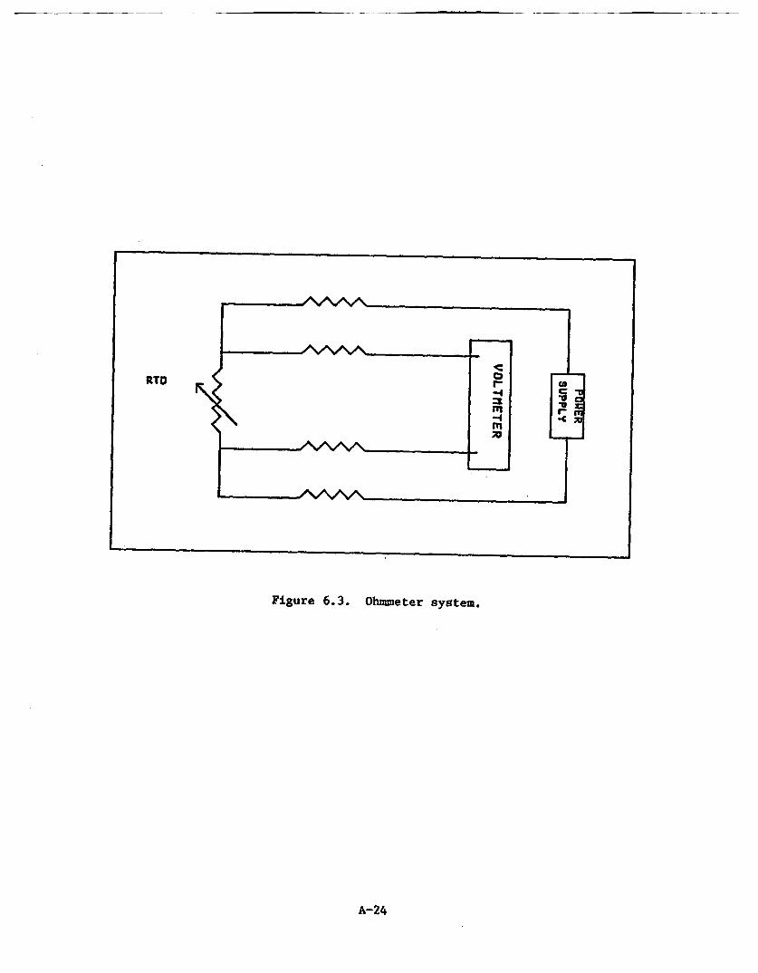
The ohmmeter system is shown in Figure 6.3. Two of the four leads areconnected to a constant current power supply and two are connected to avoltage measuring system. Ohm's law is used to provide the sensor'sresistance.
6.2 Lead Wire Effects
Lead wires add significant resistance to PRT circuits unless the wiresare very short. Consequently, it is essential to eliminate lead wireresistance contributions by appropriate instrumentation or wiring approaches.In order to permit lead wire compensation, PRTs are built in three-wire andfour-wire configurations. The common configurations are shown in Figure 6.4.
The three-wire configuration is used in bridge circuits as illustrated inFigure 6.5. This arrangement places one lead wire in each of the two opposingarms of the bridge. In this case, the bridge equation is:
A-21

Figure 6.1. Passive Wheatstone bridge circuit.
A-22
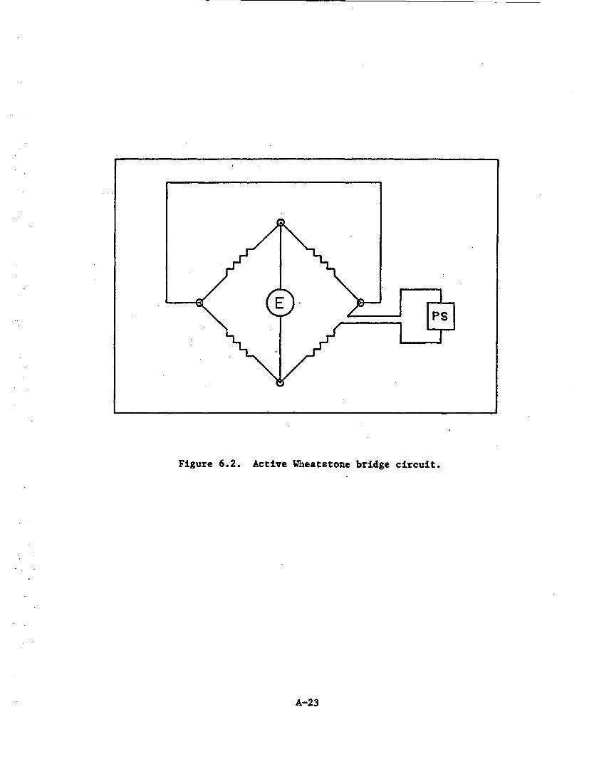
Figure 6.2. Active Wheatstone bridge circuit.
A-23
-
RTD
Figure 6.3. Ohmmeter system.
A-24

(a) 2 wire
(b) 3 wire
(c) 4 wire
(d) 2 wirewith dummy V
Figure 6.4. Lead wire configuration.
A-25

RTDAss.OM bI
Figure 6.5. Wheatstone bridge circuit with 3 wireconfiguration.
RTDAss*nb IV
Figure 6.6. Wheatstone bridge circuit with 4 wireconfiguration.
A-26

RE= Eo (R + RT + RLM)(R + RL) (ET-RS) (17)
Comparison with Equation 16 reveals that the lead wire resistances onlycontribute to the coefficient of the main temperature-dependent term. This isjust a gain factor which is handled by calibration of the bridge.
The dummy lead four-wire configuration is shown in Figure 6.6. As forthe three-wire configuration, this arrangement places the lead wires inopposite arms of the bridge. The bridge equation for this case is the same asEquation 17 except that RL is replaced by 2RL in the factors in the equation.
In the ohmmeter measurement system (see Figure 6.3), one lead on eachside of the PRT is connected to a constant current power supply. The tworemaining leads are used to monitor the voltage drop across the PRT. Sincethe voltage is measured with an instrument having high input impedance, thereis ipsignificant current flowing in the measuring circuit, and consequently,insignificant voltage drop. In this case, zero and span are set by adjustingthe bias and gain of the amplifier.
6.3 BridRe Nonlinearities
Ideally, a bridge would provide a voltage signal proportional to thePRT's resistance. That is
E - A + BRT (18)
Actual bridges have slight nonlinearities. For example, Equation 16 may berewritten in a form which is similar to Equation 18:
-E EoRRs EOR 9(R + RT)(R + R (R + RT)(R + R) (19)
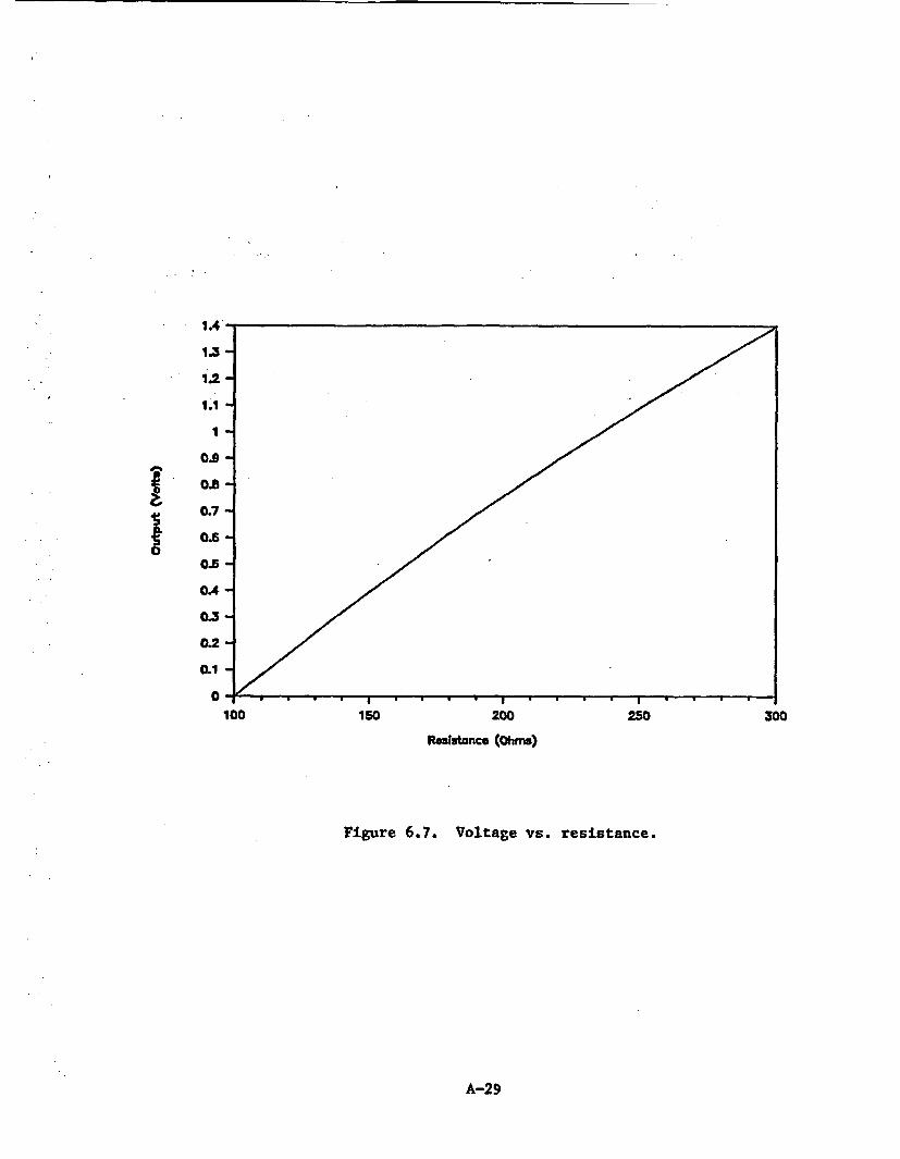
If the bracketed terms were constant, then the. voltage-resistance relationwould be linear. The presence of the RT term in the denominator makes thecoefficients vary with PRT resistance. npractice, the effect of variationsin RT can be minimized by building bridges with R large.
A-27

For example, Figure 6.7 shows the voltage vs resistance for a bridge withR = 1000 ohms, Rs - 100 ohms, and E - 10 volts.
6.4 Instrumentation Linearity
Amplifiers are used to increase voltages, and transmitters are used toprovide current signals in proportion to voltage signals. These operationswould be error-free only if the operations performed were perfectly linear.Amplifiers and transmitters are adjusted by setting zero and span.Consequently, the errors at two points are determined by the uncertainties inthe adjustments at those points, and the errors at other points areadditionally affected by the instrument's nonlinearity.
6.5 AnaloR-to-DiRital Conversion
Analog-to-digital conversion is required for systems which includedigital readouts or computer processing of temperature) signals. Theuncertainty due to analog-to-digital conversion is:
AT = 2-N (SPAN) B (20)
where
AT temperature uncertainty,
N = number of bits in analog-to-digital conversion,
SPAN span setting for temperature (OC), and
B - tolerance on analog-to-digital conversion (bits).
For example, the minimum uncertainty ( B - 1) for a twelve bit analog-to-digital converter is 0.10'C for a 400'C span (wide range) and 0.O1C for a50'C span (narrow range).
A-28
1.4-
1.3
1.1
1.
0. -/
0.7
0.6
0.3-
0.1
Or , . . . .,.... ..........
100 150 200 250 300
Reststonce (Ohnma)
Figure 6.7. Voltage vs. resistance.
A-29

6.6 Tuning
Adjustments of zero and span have been mentioned several times inprevious sections. This standard procedure suffers additional deficienciesbecause a PRT is fundamentally a three-parameter instrument (RO, a, and a areneeded to describe the sensor calibration). Consequently, a two-parameteradjustment only provides approximate matching of the instrumentation to thesensor. To use a two-parameter adjustment for a three-parameter device, onlytwo approaches are possible:
1. Ignore the error (adjust the zero and span to minimize end-point errors or maximum error); or
2. Build the instrument with a fixed value for the thirdparameter (6) which represents a typical value. The othertwo parameters (RO and a) are adjustable.
A-30

7. PRT DEGRADATIOIN
In spite of the importance of measurement accuracy of PRTs, there havebeen very few reported experimental studies of PRT degradation. Tests on onlya few hundred sensors provide the basis for assessing the performance ofhundreds of thousands of PRTs used in industrial processes. Furthermore, manyof the tests ran for only short time spans (days to weeks). Large errors havebeen observed (i.e. 25-C at 650C), but it should be noted that errors formost of the sensors' tested were much smaller (generally less than 0.05C).However, it is important to know the maximum likely error in activities whichrequire worst-case evaluation (accident analysis, replacement scheduling,calibration scheduling, etc.).
Tests have also been performed to assess another known error mechanism inPRTs, thermal hysteresis. Thermal hysteresis errors are those which occur asthe PRT experiences temperature changes over some range. The hysteresis erroris dependent on the path of varying temperatures experienced by the PRT.Errors as large as 0.31C were observed.
The postulated physical basis for the known drift and hysteresis effectsare summarized below. Ideally, experience and knowledge about PRT degradationwould permit a quantitative assessment of drift rates under given operatingconditions. Unfortunately, even the qualitative basis for PRT degradation issomewhat conjectural and quantitative predictions of the performance of aspecific sensor is not possible. The following descriptions provide currentconceptions of the mechanisms involved.
7.1 Strain
To achieve ruggedness, platinum wires or films in industrial PRTs aresupported by attachment to an insulating structure over all or part of theirlengths. The platinum and *the insulator have different thermal expansioncoefficients, so the platinum experiences stress when temperatures change.The resistance increases when the platinum is in tension and decreases when itis in compression. For small temperature changes, the stress is elastic, andconsequently, reversible. This causes the PRT to have an altered value of aand makes the Callendar-van Dusen equation inappropriate as a fittingequation.
For large temperature changes, plastic deformations occur, and the effectis not reversible. The plastic deformation is essentially a work hardeningeffect which is characterized by an increase in internal energy of the metal.This internal energy can be relieved by annealing. At the annealing
A-31

temperature, the atoms in the lattice become more mobile and the internalenergy drops to a stable condition. For platinum, annealing takes place attemperatures above 400'C. Hysteresis has been explained as the result ofplastic deformation and friction between the sensor and its mounting whichdepends on the direction of relative motion between the metal and themounting. For example, consider a wire attached to a mounting with a smallerthermal expansion coefficient than platinum. As the sensor cools, the wireshrinks more than the mounting and tensile stress occurs in the metal andplastic deformation occurs. When the sensor is heated again, the stressreverses and becomes compressive. However, the frictional resistance tomotion is dependent on the direction of motion of the metal relative to themounting. Therefore, the relief of the tensile stress has a differenttemperature dependence on heating than did the creation of the stress duringcooling. Consequently, the R vs T behavior demonstrates hysteresis.
7.2 Oxidation
The formation of PtO2 on the surface of platinum metal increases theresistance of the element at any temperature. Basically, surface oxidationreplaces a fraction of the conductor's cross section with insulating material.In essence, the radius of the conductor is reduced by the thickness of theoxide. Oxidation effects have been observed to change the calibration ofstandards-grade PRTs up to O.05C. No studies of this effect have beenpublished for industrial PRTs.
7.3 Contamination
One way to avoid oxidation is to build PRTs with reducing atmospheresinside the sheath. However, this leads to another degradation effect - metalion migration. At temperatures above 500'C, metal ions migrate from the metalsheath to the platinum where they interact metallurgically and cause a shiftin R0, and a lowering of a. Changes of Ro of as large as 0.5% have beenreported. This gives an ice point measurement error of 1.31C.
7.4 QuenchinR
Annealing at temperatures above 400eC is commonly used to eliminatestrain effects in PRTs. However, proper annealing requires slow cooling.Rapid cooling causes quenched-in lattice defects. These defects shift Ro andreduce a.
A-32

7.5 Grain Growth
The performance of a PRT depends on the condition of the crystal latticeof the metal. Grain growth occurs in platinum at temperatures above about4200C after long durations of exposure at these temperatures. When metals areheated after plastic deformation, grain growth occurs. The grain boundariesare weak points in the wire and shock or vibration can cause grain boundarysliding. This increases the electrical resistance of the wire and affects thesensor's calibration.
7.6 Cold Working
Mechanical shock and vibration can cause cold working of metals. Thiswork hardening effect alters the lattice structure of the metal and affectsits R vs T performance. Cold working can be removed by annealing.
7.7 Insulation Break Down
The electrical shunting problem due to inadequate insulation resistancewas discussed in Section 5.3. Insulation resistance changes due to moisturecan change during sensor life, so insulation resistance change is a possibledegradation mechanism. If the seal at the head of the sensor is imperfect, orif cracks or holes exist along the sensor sheath, then water can enter orleave the PRT. Operation of a PRT for extended time at elevated temperaturesgives two opposing effects:
1. Seals dry out, shrink, crack, and leak;
2. The higher temperature inside the PRT causes the water vaporto diffuse out of the sensor.
In general, the effect of moisture on insulation resistance is a concern inPRT operation. Fortunately, a resistance measurement between one of the PRTleads and ground can be used to check for this problem. The resistance ismeasured with an instrument which applies 50 to 100 vdc across the PRT. Thetest duration must be sufficient to allow polarization of the water tosaturate.
A-33

-
8. BURN-IN 0 PRTs
Typically, PRTs are built and calibrated long before installation in aplant. The elapsed time may be as long as years. In principle, the sensorsare treated carefully and no shock or vibration effects are induced.Furthermore, it is usually assumed that the sensor manufacturer has done agood job of annealing and minimizing design-related strain effects. Theseassumptions may be valid, but because of the importance of accuratetemperature measurement in nuclear power plants, it may be prudent toimplement a simple burn-in test to check the pre-installation condition of thePRTs. A possible burn-in program is:
1. Check calibration. A four-point check should be performed(at approximately 0oC, 100°C, 200'C, and 300'C). The four-point calibration will permit assessment of the conformityof the R vs T relation to the Callendar-van Dusen equation.Departure from conformity is a clue that platinum strain orchemical contamination is present. Also, the calibrationshould involve seven measurements (0°C, 100°C, 2001C, 300'C,2001C, 1001C, and 0C). This would reveal strain-inducedhysteresis.
2. Anneal. Bring the PRT to 450*C for 24 hours, then coolslowly.
3. Repeat the calibration as in Step 1. This will show whetherthe PRT is susceptible to strain or whether the sensororiginally had quenched-in or grain growth defects.
4. Install in a furnace at 3001C for two weeks.
5. Repeat the calibration as in Step 1. The two-week durationwas selected as a reasonable period to look for long-termproblems such as insulation break down.
A-34

9. PRT CBKCMG, RECOVERY, AND RECALIBRATION
After installation in a plant, the concern about decalibration begins.It is inappropriate to assume that PRTs automatically give accurate
measurements after extended use. PRTs are generally excellent sensors, but
they are not infallible. The in-plant checking involves the following:
1. Cross checking. Redundant sensors are used in nuclearplants. Limited information on sensor drift is availablethrough comparison of sensor readings. However, foridentical sensors, there is always the possibility of commonmode degradation. Ideally, multiple sensors based ondiverse measurement principles (PRTs and thermocouples)should be available. If this is not done, the next bestoption is multiple PRTs from different manufacturers. Thisguards against design-related or manufacturing-relatedcommon mode problems.
2. Insulation resistance. The insulation resistance is easilymeasured. The measurement error can be estimated usingEquation 15. When the estimated error reaches some level(i.e. O.1C), the sensor should be replaced.
3. Thermoelectric effect. While errors due to thermoelectricvoltages are not due to degradation of the PRT, it is aworrisome effect which is susceptible to simple testing.Thermoelectric effects cause changes in the indicatedtemperature when leads to the transmitters are reversed.The lead-reversal test should be performed periodically(i.e. quarterly), and the PRT should be replaced or thewiring should be corrected if the error is greater than agiven tolerance (e.g. O.10C).
The only established way to check PRT accuracy is to remove and calibratethem. In-situ calibration methods are under development, but they have notyet been qualified for field applications. Some of the PRTs should be removedand calibrated every shutdown. The remaining PRTs can be evaluated by crosschecking against the recently-calibrated PRTs.
If a PRT is found to have decalibrated, it may still be possible to useit again in the plant. This is desirable because of the high cost of PRTs fornuclear plant safety systems. If the calibration is restored by annealing at450'C, then the PRT may generally be considered "as good as new."
A-35
10. SUoHM OF FINDGS AND ECOMEDATIONS
Errors in temperature measurements with platinum resistance thermometersused in nuclear power plants are likely to be comparable to, or greater thantolerances currently required (as small as O.1C). This is true at initialsensor installation, and the concern increases with time in operation.
The actions recommended as a result of this investigation are:
1. Re-examine tolerances on temperature measurements. Some areextremely tight and probably do not reflect real needs orreal capabilities of modern temperature sensors.
2. Initiate a burn-in program for new sensors.
3. Initiate a program of routine, simple tests to check forsensor problems.
4. Initiate a program of scheduled sensor removal andrecalibration.
5. Develop a better data base of information about degradationmechanisms, their magnitudes, and their rates. This willinvolve theoretical work, single effects experiments, andlong-term testing of typical PRTs.
6. Initiate a policy of avoiding a single sensor design inmaking redundant measurements.
A-36

NRC FORM 235NRC41 U LNUCLEAR REGULATORv COAUdI. REPORT NLUSER tntdh VIOG ddvLAratm W.ae
3201320 BIBUOGRAPHIC DATA SHEET NUREG/CR-4928SEE INSTRUCTIONS ON THE REVERSE.
2 TITLE AND SUBTITLE 3 LEAVE SLANK
Degradation of Nuclear Plant Temperature Sensors
4. DATE REPORT COMPLETED
MONTH | YEAR
l, AUTHORISI May 1987
H.M. Hashemian, K.M. Petersen, T.W. Kerlin,e.DATEREPORTISSUEDR.L. Anderson, K.E. Holbert MONTH | YEAR
June 19877. PERFORMING ORGANIZATION NAME AND MAILING ADDRESS flodudfte C SO. PROJECTITASKAORK UNIT NUMBER
Analysis and Measurement Services Corporation (AMS) 9. FIN OR GRANT NUMBER
9111 Cross Park Drive, N.W.Knoxville, TN 37923-4599 D 1712
10 SPONSORING ORGANIZATION NAME AND MAILING ADDRESS toV* ZO Code) 1 1,. TYPE Of REPORT
Division of EngineeringOffice of Nuclear Regulatory Research TechnicalU.S. Nuclear Regulatory Commission BSepRIODCOVEREr 301986t
Washington, DC 20555 September 30, 1986 toApril 30, 1987
12. SUPPLEMENTARY NOTES.
13. ABSTRACT 1200 Ft dw iBu)
A program was established and initial tests were performed to evaluate long term per-formance of resistance temperature detectors (RTDs) of the type used in U.S. nuclearpower plants. The effort addressed the effect of aging on RTD calibration accuracyand response time. This Phase I effort included exposure of thirteen nuclear safetysystem grade RTD elements to simulated LWR temperatures. Full calibrations were per-formed initially and monthly, sensors were monitored and cross checked continuouslyduring exposure, and response time tests were performed before and after exposure.Short term calibration drifts of as much as 1.8°F (1lC) were observed. Response timeswere essentially unaffected by this testing.
This program shows that there is a sound reason for concern about the accuracy oftemperature measurements in nuclear power plants. These limited tests should beexpanded in a Phase II program to involve more sensors and longer exposures to simu-lated LWR conditions in order to obtain statistically significant data. This data isneeded to establish meaningful testing or replacement intervals for safety system RTDs.An important corollary benefit from this expanded program will be a better definitionof achievable accuracies in RTD calibration.
This report concludes a six-month Phase I project performed for the Nuclear RegulatoryCommission under the SBIR program.
Y. -.....
14. DOCUMENT ANALYSIS - a. KEYWORDSIDESCRIPTORS
resistance temperature detectors (RTDs)temperature measurementsSBIR Program
b, IDENTIFIERSIOPEN-ENDED TERMS
1,AVAILABILITYSTATEMENT
Unlimited
I&.SECURITYCLASSIFICATION
(Thai Peg
Unclassified(This JPerd
Unclassified17. NUMBER OP PAGES
18. PRICE
*U.S. GOVCRNMET PRINTING orrIcE0987-181-682S60138