Embed Size (px)
Citation preview

© Childerley Solutions 2002 1
GSM Radio Network Optimisation v1.4Page 1© Telecom network Consultants Ltd 2002
GSM Radio Network GSM Radio Network OptimisationOptimisation
February 2006February 2006
Trainer:Trainer: Mr Neville Hawkins Mr Neville Hawkins

© Childerley Solutions 2002 2
GSM Radio Network Optimisation v1.4Page 2© Telecom network Consultants Ltd 2002
•• IntroductionIntroduction–– Definition Definition –– ObjectivesObjectives–– Types of optimisationTypes of optimisation–– Network expansionNetwork expansion–– Interfacing groupsInterfacing groups–– Optimisation strategyOptimisation strategy
•• System basicsSystem basics–– GSM air interface GSM air interface –– Measurements Measurements
•• BSS ParametersBSS Parameters–– Idle modeIdle mode–– Measurement filteringMeasurement filtering–– Power ControlPower Control–– Locating (Handover)Locating (Handover)
Contents
••Quality assessmentQuality assessment––Network performance Network performance measurementsmeasurements––Field measurementsField measurements
••Optimisation measuresOptimisation measures––Antenna adjustmentsAntenna adjustments––Frequency and interference planningFrequency and interference planning––Neighbour list planningNeighbour list planning––Common problems Common problems ––Advanced techniquesAdvanced techniques
••OrganisationOrganisation––TimetablesTimetables––TeamsTeams––PreparationPreparation––DatabasesDatabases––Implementation proceduresImplementation procedures

© Childerley Solutions 2002 3
GSM Radio Network Optimisation v1.4Page 3© Telecom network Consultants Ltd 2002
Contents
� Introduction• System Basics• BSS Parameters • Quality Assessment• Optimisation Measures• Organisation

© Childerley Solutions 2002 4
GSM Radio Network Optimisation v1.4Page 4© Telecom network Consultants Ltd 2002
Introduction
• Definition • Objectives• Types of optimisation• Network expansion• Interfacing groups• Optimisation strategy

© Childerley Solutions 2002 5
GSM Radio Network Optimisation v1.4Page 5© Telecom network Consultants Ltd 2002
Introduction
• Definition– “the process of fine tuning the radio network cost effectively, to improve the air interface performance to achieve the desired performance quality targets”
• Objectives– Minimise interference– Achieve specified GOS – Achieve other network quality targets
• Call success rate > 99%
Radio optimisation is an essential process of fine tuning the network in the most cost-effective manner in order to improve the air interface performance so that it meets the required network performance quality targets. Radio network optimisation is a process which is continuous throughout the lifetime of the network but can be subdivided into categories namely, initial (or pre-launch) and ongoing optimisation. The main objectives of optimisation are to minimise interference, achieve the required network quality target (GOS better than 1%), achieve high call success rate (99% or better), in a cost effective manner.The results of achieving this include increased revenue and maximum customer satisfaction.In order to achieve these objectives, it is necessary to define the key network performance metrics and the thresholds to be used in the analysis of the network statistics. Generally two thresholds are defined, the first is an optimisation threshold which enables worst performing cells to be identified for scheduled remedial work, while the second is a fault threshold which identifies cells with problems requiring immediate solution.

© Childerley Solutions 2002 6
GSM Radio Network Optimisation v1.4Page 6© Telecom network Consultants Ltd 2002
Introduction
• Types of optimisation
– Initial optimisation• A good radio network planning process may reduce level of optimisation at this stage
– Ongoing optimisation• Output from this stage should be fed back into the radio network planning process
– Augments/improves knowledge of radio network planners
– Improves the radio network planning
Initial Optimisation is carried out prior to and immediately following system launch and aims to maximise the ability of the network to deliver service at a predefined and acceptable level of network performance quality at commercial launch. It is also carried out immediately following the turn on of new cells for network expansion.
Ongoing Optimisation is a continuous program that aims to find and cure problems, and enhance the performance of the network during its operational lifetime.

© Childerley Solutions 2002 7
GSM Radio Network Optimisation v1.4Page 7© Telecom network Consultants Ltd 2002
Introduction
• Initial optimisation– Takes place prior to and immediately after network launch.
– Aims to maximise the ability of the network to deliver service at a predefined and acceptablelevel of network performance quality at commercial launch
– Also takes place after new cell additions
For a network roll-out, initial optimisation can sometimes be hampered by the fact that the network is under loaded. For example, capacity bottlenecks and increased capacity effects on interference can only be properly evaluated when the network is fully loaded. Therefore optimisation will continue after commercial launch, and further adjustments made as traffic grows. At the initial stage, there is a rapid improvement in network quality due to the fact that the network quality at that time is heavily influenced by simple problems (such as neighbour definitions) which are more easily solved. However, when the network is operational, the problems become more localised and are perhaps not as easy to solve. In addition, the introduction of major changes or features in the network may result in reduced quality, but rapid improvements should be realised following the resolution of such problems.When new cells are integrated into the live commercial network, initial optimisation is required to ensure that the parameter settings and handovers to neighbouring sites are correct and that no new problems are introduced. In this case, the network is loaded and therefore the optimisation is carried out in such a way as to minimise negative customer impact.

© Childerley Solutions 2002 8
GSM Radio Network Optimisation v1.4Page 8© Telecom network Consultants Ltd 2002
Introduction
• Ongoing optimisation
– Continuous program during operational life of network
– Find and cure problems
– Enhance network performance to meet performance quality targets
Ongoing optimisation takes place continuously on a network in order to improve quality performance with increased traffic loading, provide additional capacity (new channel additions or network-wide frequency re-tunes) and resolve specific problems which arise. Both these optimisation functions need a disciplined approach to network implementation, operation and quality and require well controlled and documented procedures.

© Childerley Solutions 2002 9
GSM Radio Network Optimisation v1.4Page 9© Telecom network Consultants Ltd 2002
Introduction
• Ongoing optimisation
– Network Expansion• Increasing the network capacity • Extending coverage to new areas
– Implemented in stages or at regular intervals• Addition of extra TRXs on existing cells• Addition of new sites
Expansion is an integral part of the operation of a mobile network. It is driven primarily by the actual growth of the subscriber base, which in turn is driven by the marketing strategy and the actual performance of the network as perceived by the user. It is essential to ensure that there is always enough capacity in the network to satisfy demand, and therefore, a strategy for network expansion planning is generally established at the early stages of the life of the network. The additional capacity must be introduced whilst maintaining and/or improving the quality of the network.
The growth of the radio network is therefore an ongoing process of refinements and adjustments based on a number of input parameters, most of which are not under the control of Radio Planning. They include: · The projected subscriber growth· The projected Usage in milli Erlangs (mE) per subscriber· Special Value-added-services· Special promotion plans· Types of subscriber equipment used· The projected number of mobile data users· Areas in the network requiring coverage improvements as identified by Marketing, Sales, Operations, Customer Care

© Childerley Solutions 2002 10
GSM Radio Network Optimisation v1.4Page 10© Telecom network Consultants Ltd 2002
Introduction
• Sources of information
– Network statistics• Daily/weekly – from tool such as Metrica
– Regular drive testing• Using test equipment (TEMS)
– Customer complaints• Via customer service
– Internal problem reports• Generated within the operating organisation
Network stats: is a very good source of information given that the amount of traffic in the network is high enough to provide reliable statistics. The frequency and level of detail of the report should also be set to ensure that there is sufficient information for the groups involved in the optimisation activities, and for management. Drive testing: while the traffic in the network is still in the early growing stages and not statistically reliable, it is useful to perform regular drive tests along standard defined routes. Calls of 2 minute duration should be made to generate data which can be analysed to obtain relevant stats. This practice should be continued throughout lifetime of network.Customer complaints: Although this is a good source of information, the details such as location and type of problem are sometimes imprecise. It is preferable not to have customer complaints because by the time the complaint is received, the problem has already caused inconvenience to a customer. It is better to find the problem before the customer does. Internal problem reports: staff in the organisation are encouraged to use the network and call to a service desk or answering machine (set up for the purpose) to lodge any faults they may find with the network (friendly customers!). All problems can then be forwarded to the optimisation team for investigation (after flitering by O&M).

© Childerley Solutions 2002 11
GSM Radio Network Optimisation v1.4Page 11© Telecom network Consultants Ltd 2002
Introduction
• Radio network optimisation– Network Expansion
Traffic
Quality
For a given quality target, a certain traffic level is achieved. As network traffic increases, the quality degrades as shown by the blue curve. To get the quality back to target,
Generally, network capacity can only be increased at regular intervals, not gradually. To provide additional capacity on existing sites as the number of subscribers to the service grows, extra radio channels have to be provided within each base station. When base stations have their full complement of channels, then existing cells have to be reduced in size by adding new sites. Coverage is provided to new areas by the integration of new sites. Therefore, site activation and frequency re-tunes are part of the ongoing system improvement, and all or parts of the network will need to be optimised after each site integration or frequency retune process. The network therefore requires ongoing optimisation
© Childerley Solutions 2002 12
GSM Radio Network Optimisation v1.4Page 12© Telecom network Consultants Ltd 2002
Introduction
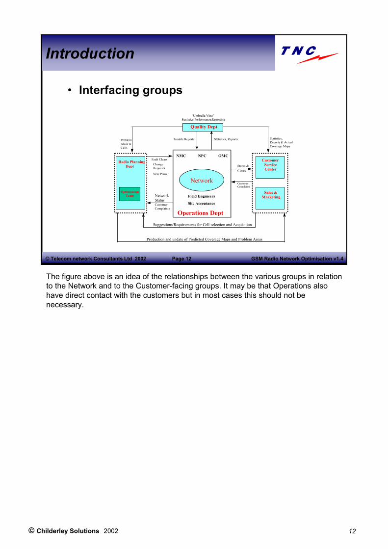
• Interfacing groups
Operations Dept
NMC
Field Engineers
OMCCustomerServiceCenter
Sales &Marketing
Radio PlanningDept
‘Umbrella View’Statistics;Performance;Reporting
ProblemAreas &Cells
Statistics,Reports & ActualCoverage Maps
Network
Site Acceptance
Status &Clears
CustomerComplaints
CustomerComplaints
ChangeRequests
Fault Clears
NetworkStatus
New Plans
Suggestions/Requirements for Cell-selection and Acquisition
Production and update of Predicted Coverage Maps and Problem Areas
Quality Dept
OptimisationTeam
Trouble Reports Statistics, Reports
NPC
The figure above is an idea of the relationships between the various groups in relation to the Network and to the Customer-facing groups. It may be that Operations also have direct contact with the customers but in most cases this should not be necessary.

© Childerley Solutions 2002 13
GSM Radio Network Optimisation v1.4Page 13© Telecom network Consultants Ltd 2002
Introduction
• Optimisation strategyPhase1: Preparation
Project plan, databases,Team/interfaces, test equipment, performance targets/thresholds
Phase2: Cluster definitionDefine clusters, generate input data (site data, maps, plots, neighbour lists, BSS parameters )
Phase3: Initial optimisationBasic site checks, cluster verification, network tuning
Phase4: Ongoing optimisationMeasurements, data analysis, solution proposal, solution implementation, verification of solution
Phase5: Database maintenance
Update all databasesFeedback results
As required for any successful project, and in particular for network optimisation, good planning and preparation are essential requirements. The optimisation campaign may be sub divided into the following stages: Phase 1: Preparation: definition of project plan, creation of database s, definition of
project team and interfaces, provision of measurement equipment/tools, generation of performance targets/thresholds, creation of optimisation guidelinesPhase 2: Cluster definition: identification and definition of BS clusters for optimisation, generation and/or collation of input data for the cluster (site data, maps, plots, neighbour lists, BSS parameters) Phase 3: Initial optimisation: site validation (basic site checks), clu ster verification, network tuning Phase 4: Ongoing optimisation: diagnostic measurements (to include test data, metrica statistics, customer complaints), identification of problems and proposal of solutions, implementation of solutions, verification of improvement in network performancePhase 5: Database maintenance: update of optimisation and other plannin g databases.

© Childerley Solutions 2002 14
GSM Radio Network Optimisation v1.4Page 14© Telecom network Consultants Ltd 2002
Introduction -review
• Definition • Objectives• Types of optimisation• Network expansion• Interfacing groups• Optimisation strategy

© Childerley Solutions 2002 15
GSM Radio Network Optimisation v1.4Page 15© Telecom network Consultants Ltd 2002
Contents
• Introduction �System Basics• BSS Parameters • Quality Assessment• Optimisation Measures• Organisation

© Childerley Solutions 2002 16
GSM Radio Network Optimisation v1.4Page 16© Telecom network Consultants Ltd 2002
GSM basics
Mast & antennas
MSC
Point ofInterconnection
BaseTransceiverStation
BTS
Base StationController
BSC
VLR
HLR
AUC
Home Location Register
AuthenticationCentre
MobileSwitchingCentre
EIR Equipment IdentityRegister
OMC/NMC Operations & Maintenance Centre/Network Management Centre
POI
Mobile Station
MS
VisitorLocationRegister
BSS
OSS
NSS
GSM System Architecture
A GSM network is a Public Land Mobile cellular Network (PLMN). It uses a network of radio transmitters to transmit radio signals over the designated service area. The radio signals are digitally encoded. This allows more services and greater security than analogue systems. The Base Station Subsystem provides the distribution function of the network. The base transceiver stations provide the actual radio link with the mobiles used by the subscribers. The BSS has a standard interface so that it is possible to connect to different types of switching centresThe Network and Switching Subsystem is responsible for handling all the switching and routing functions. The MSC does the actual switching, whilst the HLR/VLR store the subscriber data. The AUC and the EIR provide security of access to the network.The Operations Sub System is the operating nerve centre that monitors the various BSS in the network, whilst the NMC is able to monitor the NSS as well as the BSSs.
© Childerley Solutions 2002 17
GSM Radio Network Optimisation v1.4Page 17© Telecom network Consultants Ltd 2002
GSM basics
• GSM Interfaces
TO PSTN
BSC
Um Radio
Interface
BSS
TRAUNSS
Abis
InterfaceA-InterfaceAter
InterfacePSTN
Interface
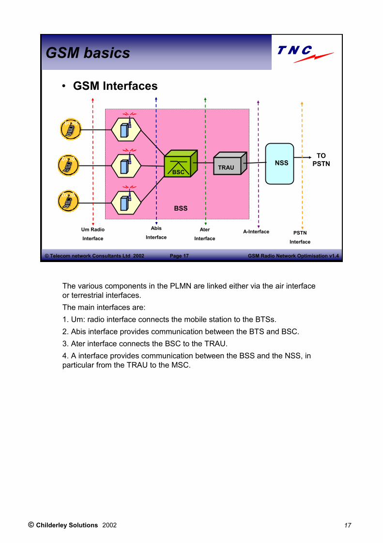
The various components in the PLMN are linked either via the air interface or terrestrial interfaces. The main interfaces are:1. Um: radio interface connects the mobile station to the BTSs.2. Abis interface provides communication between the BTS and BSC.3. Ater interface connects the BSC to the TRAU.4. A interface provides communication between the BSS and the NSS, in particular from the TRAU to the MSC.
© Childerley Solutions 2002 18
GSM Radio Network Optimisation v1.4Page 18© Telecom network Consultants Ltd 2002
Contents
• System Basics�GSM channels
�Spectrum allocation�Access scheme�Frame structures�Physical channel�Logical channels�Channel mapping (logical onto physical)
– Measurements

© Childerley Solutions 2002 19
GSM Radio Network Optimisation v1.4Page 19© Telecom network Consultants Ltd 2002
GSM Air interface
• GSM standards – 05.01: Physical layer on the radio path: general description
– 05.02: Multiplexing and multiple access on the radio path
– 05.03: Channel coding – 05.04: Modulation – 05.05: Radio transmission and reception – 05.08: Radio subsystem link control – 05.10: Radio subsystem synchronisation
The GSM standards are available from the Internet. If they were printed out they would use and enormous a mount of paper. Many are to do with fixed networking and with detailed protocols. The ones mainly relevant to the radio interface are the “05 series”. It is thoroughly recommended that radio planners and optimisation engineers read the 05 series specifications entirely.

© Childerley Solutions 2002 20
GSM Radio Network Optimisation v1.4Page 20© Telecom network Consultants Ltd 2002
GSM Air interface
• Spectrum Allocation
– 900 MHz band
– 1800 MHz band
890 MHz
915MHz
935 MHz
960 MHz
MS Transmit BS Transmit
MS Transmit BS Transmit
1710 MHz
1785MHz
1805 MHz
1880 MHz
The spectrum allocation for Standard GSM 900 Band is890 - 915 MHz: mobile transmit, base receive;935 - 960 MHz: base transmit, mobile receive.
The Extended GSM 900 Band, E-GSM (includes Standard GSM 900 band) is:880 - 915 MHz: mobile transmit, base receive;925 - 960 MHz: base transmit, mobile receive.
The allocation in the GSM 1800 Band is 1710 - 1785 MHz: mobile transmit, base receive;1805 - 1880 MHz: base transmit, mobile receive.

© Childerley Solutions 2002 21
GSM Radio Network Optimisation v1.4Page 21© Telecom network Consultants Ltd 2002
GSM Air interface
• The ARFCN– Channel bandwidth is 200kHz
GSM 900 F-DL(n) = 890 + 0.2*n 1 ≤ ≤ ≤ ≤ n ≤ ≤ ≤ ≤ 124 F-UL(n) = F-DL(n) + 45
E-GSM 900 F-DL(n) = 890 + 0.2*n 0 ≤≤≤≤ n ≤ ≤ ≤ ≤ 124 F-UL(n) = F-DL(n) + 45
F-DL(n) = 890 + 0.2*(n - 1024) 975 ≤≤≤≤ n ≤≤≤≤ 1023GSM 1800 F-DL(n) = 1710.2 + 0.2*(n - 512) 512 ≤≤≤≤ n ≤≤≤≤ 885 F-UL(n) = F-DL(n) + 95
935.2 MHz (n=1)
200 KHz 200 KHz
890.2 MHz (n=1)
MS Transmit BS Transmit
45 MHz
Each frequency carrier or channel has a bandwidth of 200kHz. The carrier frequency is designated by the Absolute Radio Frequency Channel Number (ARFCN).There are 124 channels in the standard 900 MHz band, and 374 in the 1800 MHz band. (although there are 125 channels in the 25 MHz at 900MHz band and 375 in the 1800MHz band, the lowest channel is not used to prevent interference with nearby non-GSM systems). The Mobile to Base Station path is referred to as the Uplink (UL), and the Base Station to Mobile path is the Downlink (DL).Therefore, one ARFCN comprises one Uplink frequency and a corresponding Downlink frequency.

© Childerley Solutions 2002 22
GSM Radio Network Optimisation v1.4Page 22© Telecom network Consultants Ltd 2002
GSM Air interface
• Access scheme – TDMA with FDMA
200 kHz
TS0 TS1 TS3 TS4 TS5 TS6 TS7TS2
577µµµµs
TS0 TS1 TS3 TS4 TS5 TS6 TS7TS2
TS0 TS1 TS3 TS4 TS5 TS6 TS7TS2
TS0 TS1 TS3 TS4 TS5 TS6 TS7TS2
Time
Frequency
f1
f2
f3
f4
TDMA Frame (4.615 ms)
The 200 KHz spectrum is divided in time into 8 slots. Each of the 8 slots is called a Timeslot, and its duration is 0.577ms.

© Childerley Solutions 2002 23
GSM Radio Network Optimisation v1.4Page 23© Telecom network Consultants Ltd 2002
GSM Air interface
• TDMA frame structures – Timeslot (15/26 ms)– Frame:
• 8 timeslots (TS0 - TS7)– Multiframe
• 26 frames (FN0 - FN25)• 51 frames (FN0 - FN50)
– Superframe• 51 * 26-frame multiframes• 26 * 51-frame multiframes
– Hyperframe• 2048 superframes
The 200 KHz spectrum or frame is divided in time into 8 slots. Each of the 8 slots is called a Timeslot, and its duration is (15/26ms) 0.577ms. The duration of the frame is 8*0.577=4.615ms.
Each frame has a unique number called the Frame Number (FN), starting from 0. A frame structure/hierarchy is important in order to give the BTS an internal clock system. This clocking system is used for other functions such as network access, logical channel configuration etc.
A 26-frame multiframe is used to carry Traffic channels (TCH) and associated control channels (SACCH). The 51-frame multiframe is used for control channels exclusively.

© Childerley Solutions 2002 24
GSM Radio Network Optimisation v1.4Page 24© Telecom network Consultants Ltd 2002
GSM Air interface
• TDMA frame structures
0 1 3 4 5 6 72FN0
0 1 3 4 5 6 72 0 1 3 4 5 6 72FN1 FN50
0 1 3 4 5 6 72FN25
0 1 3 4 232 24 25 0 1 3 42 48 49 50
26-frame MF 51-frame MF
0 1 3 4 232 24 25
0 1 3 42 48 49 50 51*26-Multiframe Superframe
25*51-Multiframe Superframe
0 1 3 42 2045 2046 2047
Hyperframe: 2048 Superframes
© Childerley Solutions 2002 25
GSM Radio Network Optimisation v1.4Page 25© Telecom network Consultants Ltd 2002
Exercise!
• Given• TDMA frame period = 4.615ms
– Calculate the periods for each• Multiframe• Superframe• Hyperframe

© Childerley Solutions 2002 26
GSM Radio Network Optimisation v1.4Page 26© Telecom network Consultants Ltd 2002
GSM Channels
• Channel types– Defined in GSM 05.02
– Physical channel• Frequency and timeslot• HSN and MA and MAIO
– Logical channels• Speech (e.g. TCH/FS, TCH/HS)• Data (e.g. TCH/F9.6)• Control (e.g. BCCH, SDCCH, SACCH etc)
GSM Specification 05.02 defines all the channel types. There are two categories: Logical and Physical. Physical channels are defined by the frequency or frequency sequence and the timeslot number, while logical channels by the kind of information they carry.
There are various kinds of logical channel, broadly speaking traffic and control. Traffic may be data or voice traffic. It is not possible to carry data over a voice channel (unlike with an analogue line).

© Childerley Solutions 2002 27
GSM Radio Network Optimisation v1.4Page 27© Telecom network Consultants Ltd 2002
GSM Channels
• Physical channel - Bursts– Information carried on physical channels is transmitted in bursts
– The modulation scheme is GMSK• Gaussian Minimum Shift Keying with BT=0.3• Modulation rate is 270.83 kb/s (=1625/6 kb/s)
– Corresponds to 156.25 bits in the timeslot• No amplitude modulation• Gives minimum spectrum requirements• Enables constant output power to be used
Timeslots transmit bursts of data. Five types are defined, four full ones and one short burst.
A burst is the information or physical content (speech or data) transmitted during one timeslot - it is a period of the RF carrier that is modulated by a data stream. Bursts have very precise timing characteristics, so that all network components know exactly when to transmit and when to receive. The size of the burst depends on the type of data that is transmitted. One burst contains a maximum of 156.25 bits, the odd 0.25 bit being due to a guard period of 8.25 bits duration (30µs).
Where no data is required to be conveyed, no burst is transmitted and the timeslot is empty.Reduction of BTS or MS power will result in bursts of reduced amplitude filling a timeslot.

© Childerley Solutions 2002 28
GSM Radio Network Optimisation v1.4Page 28© Telecom network Consultants Ltd 2002
GSM Channels
• Physical channel - the GSM burst
» Ref: GSM 05.05
dB
t
- 6
- 30
+ 4
8 µs 10 µs 10 µs 8 µs
(147 bits)
7056/13 (542.8) µs 10 µs(*)
10 µs
- 1+ 1
(***)
(**)
156.25 bits
A timeslot is divided into 156.25 bit periods. A particular bit period within a timeslot is referenced by a bit number (BN), with the first bit period being numbered 0, and the last (1/4) bit period being numbered 156. The bit with the lowest bit number is transmitted first.
A burst consists of sections as follows:•A guard period (approx 30µs) to prevent overlapping with adjacent bursts•A useful part containing information (147 bits)•A mid amble or training sequence, used by equaliser to calculate multipath delay and compensate.
Ramp-up and ramp-down takes place in the guard period.This is mandatory for MS transmission, but the BTS is not required to ramp up and down between adjacent bursts.

© Childerley Solutions 2002 29
GSM Radio Network Optimisation v1.4Page 29© Telecom network Consultants Ltd 2002
GSM Channels
• Physical channel - Bursts
– Five types• Normal burst (NB)• Frequency correction burst (FB) • Synchronisation burst (SB)• Access burst (AB)• Dummy burst (DB)
Timeslots transmit bursts of data. There are different kinds of burst associated with different channel types.
© Childerley Solutions 2002 30
GSM Radio Network Optimisation v1.4Page 30© Telecom network Consultants Ltd 2002
GSM Channels
• Physical channel - bursts
Normal Burst
3 142 3 81/4
3 39 3964 3 81/4
8 41 36 3 681/4
Frequency Correction Burst
Synchronisation Burst
Dummy Burst
Access Burst
1 1
Tail Guard
Period
Extended Training Sequence
3 58 5826 3 81/4Encrypted Data Encrypted DataTraining
Sequence
Tail
Fixed Sequence
Encrypted Data Encrypted Data
Encrypted DataSynchronisation
Sequence
Extended Guard Period
3 58 5826 3 81/4Encrypted Data Encrypted DataTraining
Sequence
Tail
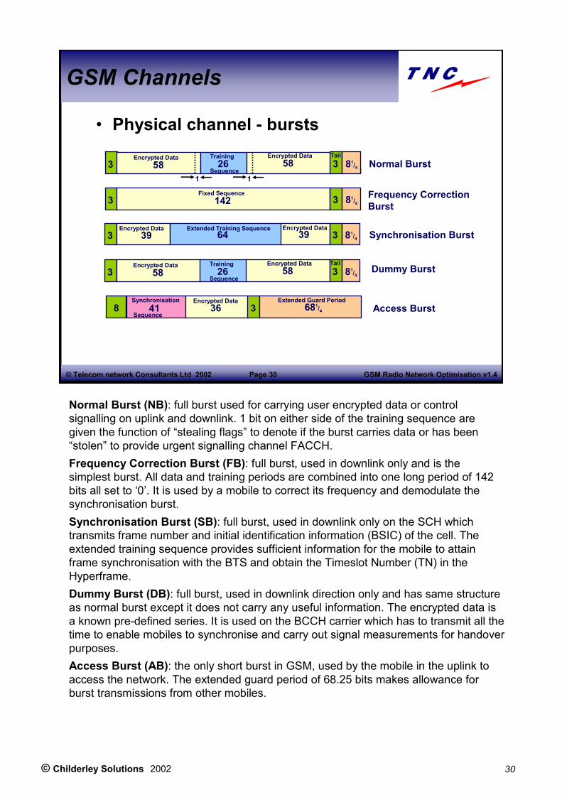
Normal Burst (NB): full burst used for carrying user encrypted data or control signalling on uplink and downlink. 1 bit on either side of the training sequence are given the function of “stealing flags” to denote if the burst carries data or has been “stolen” to provide urgent signalling channel FACCH.Frequency Correction Burst (FB): full burst, used in downlink only and is the simplest burst. All data and training periods are combined into one long period of 142 bits all set to ‘0’. It is used by a mobile to correct its frequency and demodulate the synchronisation burst.Synchronisation Burst (SB): full burst, used in downlink only on the SCH which transmits frame number and initial identification information (BSIC) of the cell. The extended training sequence provides sufficient information for the mobile to attain frame synchronisation with the BTS and obtain the Timeslot Number (TN) in the Hyperframe.Dummy Burst (DB): full burst, used in downlink direction only and has same structure as normal burst except it does not carry any useful information. The encrypted data is a known pre-defined series. It is used on the BCCH carrier which has to transmit all the time to enable mobiles to synchronise and carry out signal measurements for handover purposes.Access Burst (AB): the only short burst in GSM, used by the mobile in the uplink to access the network. The extended guard period of 68.25 bits makes allowance for burst transmissions from other mobiles.

© Childerley Solutions 2002 31
GSM Radio Network Optimisation v1.4Page 31© Telecom network Consultants Ltd 2002
GSM Channels
• Physical Channel
0 1 2 3 4 5 6 7 0 1 2 3 4 5 6 7 0 1 2 3 4 5 6 7
Timeslot156.25 bits
0.577 ms
Physical Channel
TDMA Frame
TDMA FrameDuration: 4.615msNo.of timeslots: 8Numbering: 0 – 2 715 647
(25 x 51 x 2048 –1)
TimeslotDuration: 577usNo.of bits: 156.25Numbering: 0 - 7
A TDMA Frame consists of the 8 consecutive timeslots [0,1,2,3,4,5,6,7]. The TDMA frames are numbered rigidly, because different frames carry different channels, for example a TCH and a SACCH share the same timeslot number and frequency, but are differentiated through the TDMA frame number sequence that they use.
The Physical channel is the repetition of a particular timeslot - in this example, TS 1. The repetition of TS 2 would be another physical channel, etc. etc.Therefore one RF carrier can carry up to 8 simultaneous conversations, in other words it carries transmissions from 8 different subscribers simultaneously. The Mobile or base station must transmit the information related to one call in the same timeslot until the call is terminated.
Each physical channel carries a varying number of logical channels.

© Childerley Solutions 2002 32
GSM Radio Network Optimisation v1.4Page 32© Telecom network Consultants Ltd 2002
GSM Channels
• Physical channels– Frequencies, channel allocation
• CA: the list of frequencies allocated to a cell• MA: the list of frequencies allocated to a mobile
– When frequency hopping• MAI: indexes the list of mobile frequencies
– For each TDMA frame• MAIO: offset to the MA Index to avoid two TRX in one cell using the same frequency
• HSN: Hopping sequence number
Each cell is allocated a set of frequencies. The allocation is stored in the CA (Cell Allocation). The frequencies may be hopping or not. When frequency hopping, a mobile will be allocated a set of frequencies called the MA (Mobile Allocation). The MA will be a subset of the CA.The hopping sequence generation algorithm is carefully defined in GSM 05.02. The algorithm itself generates an index (MAI) for each TDMA frame, which is used to look up from the MA list the actual frequency used in each TDMA frame. Transceivers in one cell using the same MA are each given an offset (MAIO) to the index number for each frame. This makes it impossible for two TRX in the same cell to use the same frequency in the same TDMA frame.The sequence generation algorithm uses the Hopping Sequence Number (HSN) and the TDMA Frame Number (FN) to generate the MAI. FN is effectively random for non synchronised BSs, but is the same for the cells on the same site.

© Childerley Solutions 2002 33
GSM Radio Network Optimisation v1.4Page 33© Telecom network Consultants Ltd 2002
GSM Channels
• Logical Channels– Traffic CHannels (TCH)
• Speech channels– Full rate traffic channel for speech (TCH/FS)– Half rate traffic channel for speech (TCH/HS)
• Data channels– Full rate traffic for 9.6 kbit/s data (TCH/F9.6)– Full rate traffic for 4.8 kbit/s data (TCH/F4.8)– Full rate traffic for ≤≤≤≤ 2.4 kbit/s data (TCH/F2.4)– Half rate traffic for 4.8 kbit/s data (TCH/H4.8)– Half rate traffic for ≤≤≤≤ 2.4 kbit/s data (TCH/H2.4)
GSM requires a great variety of information (data and control) to be transmitted in both uplink and downlink. The concept of logical channels is used to convey the different types of data. Therefore, to use a given channel is to transmit and receive specific bursts at specific instants in time and on specific frequencies.
Speech traffic channels may be Full Rate or Half Rate or Enhanced Full Rate. Half Rate channels only occupy half of each time slot.

© Childerley Solutions 2002 34
GSM Radio Network Optimisation v1.4Page 34© Telecom network Consultants Ltd 2002
GSM Channels
• Logical Channels– Traffic CHannels (TCH)
• Data channels
TCH
TCH/F TCH/H
TCH/H 4.8 TCH/H 2.4TCH/F 9.6
TCH/F 4.8
TCH/F 1.2
TCH/F 2.4
The Traffic channels carries either speech or data.
The Full Rate channel carries encoded information at a gross rate of 22.8 kb/s. The net rate for speech is 13 kb/s, whilst for data, the net rates are 9.6 kb/s, 4.8 kb/s, 2.4 kb/s. •TCH/F9.6: 9.6 kb/s full rate data•TCH/F4.8: 4.8 kb/s full rate data•TCH/F2.4: 2.4 kb/s full rate dataThe Half Rate channel have less coding overhead and carry encoded information at a gross rate of 11.4 kb/s, and net rates of 4.8 kb/s, 2.4 kb/s. •TCH/H4.8: 4.8 kb/s half rate data•TCH/H2.4: 2.4 kb/s half rate data
Since 9.6 kbit/s is already slow enough, few people use the 4.8k or 2.4k channels.

© Childerley Solutions 2002 35
GSM Radio Network Optimisation v1.4Page 35© Telecom network Consultants Ltd 2002
GSM Channels
• Logical Channels– Control channels
• Broadcast Channels (BCH)
• Common control channels (CCCH)
• Dedicated Control Channels (DCCH)
There are a large number of control channels defined for different purposes. The Control channels (CCH) carry signalling or synchronisation information. There are three main types of control channels:BCCH: Broadcast Control Channel: downlink only and are transmitted to all mobilesCCCH: Common Control Channel: used for a temporary period to make connections and set up other channelsDCCH: Dedicated Control Channel: used for a temporary period to make connections and set up other channels

© Childerley Solutions 2002 36
GSM Radio Network Optimisation v1.4Page 36© Telecom network Consultants Ltd 2002
GSM Channels
• Logical Channels– Control CHannels (CCH)
CCH
DCCH
SDCCH
BCCH
SCH FCCH
BCCH
FACCH
ACCH
SACCH
CCCH
RACH
PCH AGCH
(DL)
(UL)
(DL) (DL)CBCH
(DL)
(UL&DL)
BCCH: Point to multipoint, unidirectional (Downlink) channel, transmitted at constant power all the time from the BS. It carries information such as List of frequencies used in cell, cell identity, location area identity, list of neighbour cells, access control (emergency calls etc.), power control & DTX information. It includesCCCH: Point to multipoint, bi-directional (Up & Downlink) channel, used for carrying signalling data for access management functions. It includesDCCH: Point to point, directional (Up & Downlink) channel, used for carrying signalling data for call setup or for measurement and handover purposes. It includes•SDCCH: Stand Alone Dedicated Control Channel, used for data transfer to/from mobile during call setup, and for transmission of SMS•ACCH: Associated Control channel, can be associated with either a TCH or an SDCCH, and are used for the processes associated with those two channels
•SACCH: Slow Associated Control Channel, carries timing and power control information downlink to the mobile, and quality and signal strength measurements uplink to the BS.•FACCH: Fast Associated Control channel is used to implement user authentication and handovers. It is transmitted instead of a TCH, and is referred to as burst stealing - the FACCH steals the TCH burst and replaces it with its own information.
© Childerley Solutions 2002 37
GSM Radio Network Optimisation v1.4Page 37© Telecom network Consultants Ltd 2002
GSM Channels
• Logical Channels: Control channels
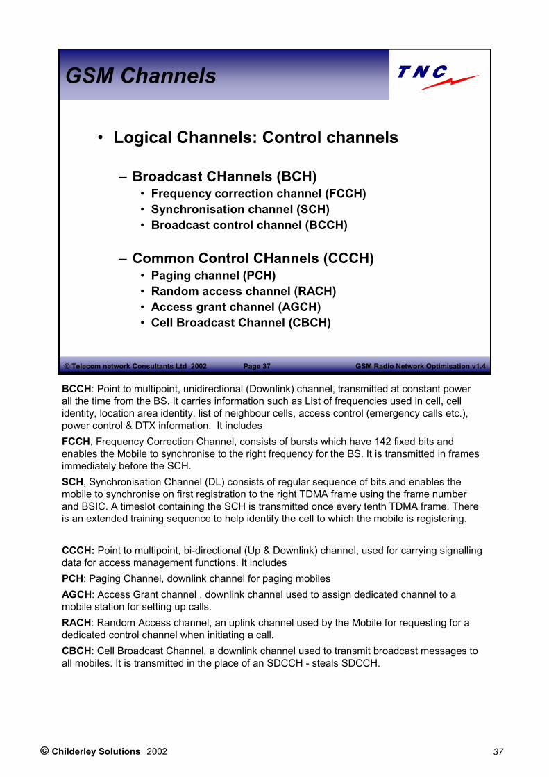
– Broadcast CHannels (BCH)• Frequency correction channel (FCCH)• Synchronisation channel (SCH)• Broadcast control channel (BCCH)
– Common Control CHannels (CCCH)• Paging channel (PCH)• Random access channel (RACH)• Access grant channel (AGCH)• Cell Broadcast Channel (CBCH)
BCCH: Point to multipoint, unidirectional (Downlink) channel, transmitted at constant power all the time from the BS. It carries information such as List of frequencies used in cell, cell identity, location area identity, list of neighbour cells, access control (emergency calls etc.), power control & DTX information. It includesFCCH, Frequency Correction Channel, consists of bursts which have 142 fixed bits and enables the Mobile to synchronise to the right frequency for the BS. It is transmitted in frames immediately before the SCH.SCH, Synchronisation Channel (DL) consists of regular sequence of bits and enables the mobile to synchronise on first registration to the right TDMA frame using the frame number and BSIC. A timeslot containing the SCH is transmitted once every tenth TDMA frame. There is an extended training sequence to help identify the cell to which the mobile is registering.
CCCH: Point to multipoint, bi-directional (Up & Downlink) channel, used for carrying signalling data for access management functions. It includesPCH: Paging Channel, downlink channel for paging mobilesAGCH: Access Grant channel , downlink channel used to assign dedicated channel to a mobile station for setting up calls.RACH: Random Access channel, an uplink channel used by the Mobile for requesting for a dedicated control channel when initiating a call.CBCH: Cell Broadcast Channel, a downlink channel used to transmit broadcast messages to all mobiles. It is transmitted in the place of an SDCCH - steals SDCCH.

© Childerley Solutions 2002 38
GSM Radio Network Optimisation v1.4Page 38© Telecom network Consultants Ltd 2002
GSM Channels
• Control channels– Dedicated Control CHannels
• Slow associated control channel (SACCH/TF)• Fast associated control channel (FACCH/TF)• Stand alone dedicated control channel (SDCCH/8)• Slow associated control channel (SACCH/C8)• Stand alone dedicated control channel, combined with CCCH (SDCCH/4)
DCCH: Point to point, directional (Up & Downlink) channel, used for carrying signalling data for call setup or for measurement and handover purposes. Dedicated channels are so called because they are dedicated to one mobile in dedicated mode (as opposed to idle mode). Dedicated control channels fall into two categories: There are “stand alone” channels and “associated” channels. The stand alone channels can be set up in their own right. SDCCH: Stand Alone Dedicated Control Channel, used for data transfer to/from BS/MS during call setup, and for transmission of SMS. Messages inc. “Layer 3” messages and indicate commands such as “Assign Channel”, “Update Location Area”, etc. The SDCCH can be combined on the same physical channel as the BCCH and CCCHs, and is time division multiplexed, or can be allocated an entire physical channel itself, depending on the traffic requirements.ACCH: Associated Control channel, can only be associated with either a TCH or an SDCCH, and are used for the processes associated with those two channels
SACCH: Slow Associated Control Channel uses a small number of timeslots occasionally to carry timing and power control information downlink to the mobile, and quality and signal strength measurements uplink to the BS.FACCH: Fast Associated Control channel is used to implement user authentication and handovers. It is transmitted instead of a TCH, and is referred to as burst stealing - the FACCH steals the TCH burst and replaces it with its own information. That is, a FACCH exists when a TCH is temporarily used for SDCCH purposes.

© Childerley Solutions 2002 39
GSM Radio Network Optimisation v1.4Page 39© Telecom network Consultants Ltd 2002
GSM Channels
• Logical Channels
Normal Burst
SDCCH
BCCH
CBCHPCH
AGCH
FACCH
SACCH
Access Burst
RACH
Dummy Burst
BCCH FCH SCH
Frequency Burst
SynchronisationBurst

© Childerley Solutions 2002 40
GSM Radio Network Optimisation v1.4Page 40© Telecom network Consultants Ltd 2002
GSM Channels
• Mapping Logical to Physical channels– Physical channel has several logical channels
• TCH/F + FACCH/F + SACCH/TF
• FCCH + SCH + BCCH + CCCH• SDCCH/8 + SACCH/C8
– “Non-combined”
• FCCH + SCH + BCCH + CCCH + SDCCH/4 + SACCH/C4
– “Combined”
• where CCCH = PCH + RACH + AGCH

© Childerley Solutions 2002 41
GSM Radio Network Optimisation v1.4Page 41© Telecom network Consultants Ltd 2002
GSM Channels
• Channel Mapping: Logical to Physical– TCH carrier
• TCH/F + SACCH/TF + FACCH/F
• 24 slots for TCH/F• 1 slot for SACCH• 1 idle slot
TCH
TCH
TCH
TCH
TCH
TCH
TCH
TCH
TCH
TCH
TCH
TCH
SACC
H
TCH
TCH
TCH
TCH
TCH
TCH
TCH
TCH
TCH
TCH
TCH
TCH
IDLE
0 1 3 4 5 6 72FN0
0 1 3 4 5 6 72FN1
0 1 3 4 5 6 72FN25
The TCH configuration comprises 24 TS where TCH/F (speech or user data) is transmitted. 1 TS for its SACCH (each TCH has an associated SACCH to convey signalling between MS and BTS in active mode), and 1 TS is idle. The TCH/F period is 120ms, chosen as a multiple of 20ms in order to obtain some synchronisation with fixed networks, especially ISDN.
If the network sets the “stealing flags” in the normal burst, a timeslot can be stolen and replaced with a FACCH to send urgent signalling data

© Childerley Solutions 2002 42
GSM Radio Network Optimisation v1.4Page 42© Telecom network Consultants Ltd 2002
GSM Channels
• Channel Mapping: Logical to Physical– BCCH carrier (non combined)
• FCH + SCH + BCCH + CCCH
– 5 TS for FCH– 5 TS for SCH– 4 TS for BCCH– 36 TS for CCCH– 1 TS is idle
FCC
HS
CH
BCC
HBC
CH
BCC
HBC
CH
CCC
HCC
CH
CCC
HCC
CH
FCC
CH
SC
HCC
CH
CCC
HCC
CH
CCC
HCC
CH
CCC
HCC
CH
CCC
HFC
CH
SC
HCC
CH
CCC
HCC
CH
CCC
HCC
CH
CCC
HCC
CH
CCC
HFC
CH
SC
HCC
CH
CCC
HCC
CH
CCC
HCC
CH
CCC
HCC
CH
CCC
HFC
CH
SC
HCC
CH
CCC
HCC
CH
CCC
HCC
CH
CCC
HCC
CH
CCC
HID
LE
0 1 3 4 5 6 72FN0
0 1 3 4 5 6 72FN1
0 1 3 4 5 6 72FN25
0 1 3 4 5 6 72FN50
With non-combined, a separate timeslot is used for eight SDCCH channels and their SACCHs.

©Childerley Solutions
200243
GSM
Radio N
etwork O
ptimisation v1.4
Page 43©Telecom
network C
onsultants Ltd 2002
GSM
Channels
•Channel M
apping: Logical to Physical–SD
CCH non com
bined (SDCCH/8 + SA
CCH/C8)
Cycle repeated after 102 TD
MA fram
es
SDCCH/4(0)
SDCCH/4(0)
SDCCH/4(0)
SDCCH/4(0)
SDCCH/4(1)
SDCCH/4(1)
SDCCH/4(1)
SDCCH/4(1)
SDCCH/4(2)
SDCCH/4(2)
SDCCH/4(2)
SDCCH/4(2)
SDCCH/4(3)
SDCCH/4(3)
SDCCH/4(3)
SDCCH/4(3)
SDCCH/4(4)
SDCCH/4(4)
SDCCH/4(4)
SDCCH/4(4)
SDCCH/4(5)
SDCCH/4(5)
SDCCH/4(5)
SDCCH/4(5)
SDCCH/4(6)
SDCCH/4(6)
SDCCH/4(6)
SDCCH/4(6)
SDCCH/4(7)
SDCCH/4(7)
SDCCH/4(7)
SDCCH/4(7)
SACCH/C4/(0)
SACCH/C4/(0)
SACCH/C4/(0)
SACCH/C4/(0)
SACCH/C4/(1)
SACCH/C4/(1)
SACCH/C4/(1)
SACCH/C4/(1)
SACCH/C4/(3)
SACCH/C4/(3)
SACCH/C4/(3)
SACCH/C4/(3)
SACCH/C4/(3)
SACCH/C4/(3)
SACCH/C4/(3)
SACCH/C4/(3)
IDLE
IDLE
IDLE
01
34
56
72 FN
00
13
45
67
2 FN1
01
34
56
72 FN
250
13
45
67
2FN
50
01
34
56
72FN
101
SDCCH/4(0)
SDCCH/4(0)
SDCCH/4(0)
SDCCH/4(0)
SDCCH/4(1)
SDCCH/4(1)
SDCCH/4(1)
SDCCH/4(1)
SDCCH/4(2)
SDCCH/4(2)
SDCCH/4(2)
SDCCH/4(2)
SDCCH/4(3)
SDCCH/4(3)
SDCCH/4(3)
SDCCH/4(3)
SDCCH/4(4)
SDCCH/4(4)
SDCCH/4(4)
SDCCH/4(4)
SDCCH/4(5)
SDCCH/4(5)
SDCCH/4(5)
SDCCH/4(5)
SDCCH/4(6)
SDCCH/4(6)
SDCCH/4(6)
SDCCH/4(6)
SDCCH/4(7)
SDCCH/4(7)
SDCCH/4(7)
SDCCH/4(7)
SACCH/C4/(4)
SACCH/C4/(4)
SACCH/C4/(4)
SACCH/C4/(4)
SACCH/C4/(5)
SACCH/C4/(5)
SACCH/C4/(5)
SACCH/C4/(5)
SACCH/C4/(6)
SACCH/C4/(6)
SACCH/C4/(6)
SACCH/C4/(6)
SACCH/C4/(7)
SACCH/C4/(7)
SACCH/C4/(7)
SACCH/C4/(7)
IDLE
IDLE
IDLE
TS1 is used for SD
CC
H in the non com
bined configuration. Each SDC
CH
has an associated SA
CC
H. For every eight S
DC
CH
TDM
A fram
es there are four S
AC
CH
frames.
The idle frames are an opportunity for the m
obile to synchroniseto neighbouring
cells and to decode their BS
IC.

©Childerley Solutions
200244
GSM
Radio N
etwork O
ptimisation v1.4
Page 44©Telecom
network C
onsultants Ltd 2002
GSM
Channels
•Channel M
apping: Logical to Physical–BCCH carrier (com
bined)•FC
CH + SC
H + B
CCH + C
CCH + SD
CCH/4 + SA
CCH/C4
Cycle repeated after 102 TD
MA fram
es
FCCH
SCH
BCCH
BCCH
BCCH
BCCH
CCCH
CCCH
CCCH
CCCH
FCCCH
SCH
CCCH
CCCH
CCCH
CCCH
CCCH
CCCH
CCCH
CCCH
FCCH
SCH
SDCCH/4(0)
SDCCH/4(0)
SDCCH/4(0)
SDCCH/4(0)
SDCCH/4(1)
SDCCH/4(1)
SDCCH/4(1)
SDCCH/4(1)
FCCH
SCH
SDCCH/4(2)
SDCCH/4(2)
SDCCH/4(2)
SDCCH/4(2)
SDCCH/4(3)
SDCCH/4(3)
SDCCH/4(3)
SDCCH/4(3)
FCCH
SCH
SACCH/C4/(0)
SACCH/C4/(0)
SACCH/C4/(0)
SACCH/C4/(0)
SACCH/C4/(1)
SACCH/C4/(1)
SACCH/C4/(1)
SACCH/C4/(1)
IDLE
FCCH
SCH
BCCH
BCCH
BCCH
BCCH
CCCH
CCCH
CCCH
CCCH
FCCCH
SCH
CCCH
CCCH
CCCH
CCCH
CCCH
CCCH
CCCH
CCCH
FCCH
SCH
SDCCH/4(0)
SDCCH/4(0)
SDCCH/4(0)
SDCCH/4(0)
SDCCH/4(1)
SDCCH/4(1)
SDCCH/4(1)
SDCCH/4(1)
FCCH
SCH
SDCCH/4(2)
SDCCH/4(2)
SDCCH/4(2)
SDCCH/4(2)
SDCCH/4(3)
SDCCH/4(3)
SDCCH/4(3)
SDCCH/4(3)
FCCH
SCH
SACCH/C4/(2)
SACCH/C4/(2)
SACCH/C4/(2)
SACCH/C4/(2)
SACCH/C4/(3)
SACCH/C4/(3)
SACCH/C4/(3)
SACCH/C4/(3)
IDLE
01
34
56
72 FN
00
13
45
67
2 FN1
01
34
56
72 FN
250
13
45
67
2FN
50
01
34
56
72FN
101
Synchronisation and frequency correction happens every tenth TD
MA
frame.
Each S
DC
CH
has an associated SAC
CH
. For every eight SD
CC
H TD
MA
frames
there are four SAC
CH
frames.

© Childerley Solutions 2002 45
GSM Radio Network Optimisation v1.4Page 45© Telecom network Consultants Ltd 2002
GSM Channels
• Call set-up– Mobile terminated
• PCH used to transmit page to mobile in all cells within the Location Area in which it was last registered in the VLR
PCH

© Childerley Solutions 2002 46
GSM Radio Network Optimisation v1.4Page 46© Telecom network Consultants Ltd 2002
GSM Channels
• Call set-up– Mobile terminated
• Mobile “hears” page and requests communication on the RACH
PCH
RACH

© Childerley Solutions 2002 47
GSM Radio Network Optimisation v1.4Page 47© Telecom network Consultants Ltd 2002
GSM Channels
• Call set-up– Mobile terminated
• Base station responds on the Access Grant Channel (AGCH), with details of a Dedicated Control Channel (SDCCH)
RACH
AGCH

© Childerley Solutions 2002 48
GSM Radio Network Optimisation v1.4Page 48© Telecom network Consultants Ltd 2002
GSM Channels
• Call set-up– Mobile terminated
• The SDCCH is used to transfer all call set-up information, e.g. authentication details, callers number (if enabled), etc.
SDCCH

© Childerley Solutions 2002 49
GSM Radio Network Optimisation v1.4Page 49© Telecom network Consultants Ltd 2002
GSM Channels
• Call set-up– Mobile terminated
• On the SDCCH, the mobile is told which traffic channel to use (frequency, hopping sequence, timeslot)
SDCCH
TCH

© Childerley Solutions 2002 50
GSM Radio Network Optimisation v1.4Page 50© Telecom network Consultants Ltd 2002
GSM Channels
• Call set-up– Mobile originated
• Rather than starting with a “downlink” page, the mobile initiates proceedings on the RACH
RACH
AGCH

© Childerley Solutions 2002 51
GSM Radio Network Optimisation v1.4Page 51© Telecom network Consultants Ltd 2002
GSM Channels
• Call set-up– Summary
Paging (PCH) -mobile
terminated onlyRandom Access Request (RACH)
Access Grant (AGCH)
Call setup (SDCCH)
Call in progress (TCH)

© Childerley Solutions 2002 52
GSM Radio Network Optimisation v1.4Page 52© Telecom network Consultants Ltd 2002
GSM Channels - Review
•• GSM channelsGSM channels–– Spectrum allocationSpectrum allocation–– Access schemeAccess scheme–– Frame structuresFrame structures–– Physical channelPhysical channel–– Logical channelsLogical channels–– Channel Mapping: Logical onto physicalChannel Mapping: Logical onto physical

© Childerley Solutions 2002 53
GSM Radio Network Optimisation v1.4Page 53© Telecom network Consultants Ltd 2002
Contents
• System Basics– GSM Channels�Measurements
• Idle mode• Dedicated mode• RxLev• RxQual• Radio Link Timer• Timing Advance

© Childerley Solutions 2002 54
GSM Radio Network Optimisation v1.4Page 54© Telecom network Consultants Ltd 2002
GSM Measurements
• Idle mode• Dedicated mode• RxLev• RxQual• Radio Link Timer• Timing Advance

© Childerley Solutions 2002 55
GSM Radio Network Optimisation v1.4Page 55© Telecom network Consultants Ltd 2002
GSM Measurements
• Downlink, idle mode– Signal level of BCCH carrier frequency– Signal level of BCCH carrier from 6 neighbours
• Uplink, idle mode– No measurements
In idle mode it is not possible to measure the Bit error rate. Also, it is not possible to measure the bit error rate of neighbours in dedicated mode.

© Childerley Solutions 2002 56
GSM Radio Network Optimisation v1.4Page 56© Telecom network Consultants Ltd 2002
GSM Measurements
• Downlink, dedicated mode– Signal level of serving carrier– Signal level of BCCH carrier from 6 neighbours– Bit error rate of serving channel
• Uplink, dedicated mode– Signal level of serving carrier– Bit error rate of serving channel

© Childerley Solutions 2002 57
GSM Radio Network Optimisation v1.4Page 57© Telecom network Consultants Ltd 2002
GSM Measurements
• Signal level, RxLevRxLev Signal0 < -110dBm1 -110 to -109dBm2 -109 to -108dBm: :: :61 - 49 to - 48dBm62 - 48 to - 47dBm63 > - 47 dBm
Signal level is represented as RxLev for transmission back to the BSC. The RxLev actually represents a signal level range, usually 1 dB. Therefore Signal levels lower than –110dBm are reported as RxLev 0, and levels higher than –47 dBm are represented as RxLev 63. Even if a test mobile can measure higher, it is still reported to the BSC as 63. Signal level higher than –110dBm but lower than –109dBm is reported as RxLev1 etc. etc.

© Childerley Solutions 2002 58
GSM Radio Network Optimisation v1.4Page 58© Telecom network Consultants Ltd 2002
GSM Measurements
• Bit Error Rate (BER(), RxQualRxQual BER range BER mean0 < 0.2% 0.14%1 0.2 to 0.4% 0.28%2 0.4 to 0.8% 0.57%3 0.8 to 1.6% 1.13%4 1.6 to 3.2% 2.26%5 3.2 to 6.4% 4.53%6 6.4 to 12.8% 9.05%7 > 12.8% 18.1%
RxQual of 4, about 2% BER, is about the limit of acceptable voice quality when not hopping. 5 is unacceptable. In a hopping system RxQual of 6 may still give acceptable speech quality. The error correction coding will restore the original data to a lower BER.

© Childerley Solutions 2002 59
GSM Radio Network Optimisation v1.4Page 59© Telecom network Consultants Ltd 2002
GSM Measurements
• Measurement reporting– Reported once every (SACCH/TCH-F multiframe)
• Every 104 TDMA frames = 480ms for TCH• Every 102 TDMA frames = 471ms for SDCCH
– 4 TDMA frames carry SACCH channel• Measurements reported on uplink• Messages sent on downlink• 2 idle frames
Measurements made by the MS on the neighbour cells are sent to the BSC on the SACCH channel.
© Childerley Solutions 2002 60
GSM Radio Network Optimisation v1.4Page 60© Telecom network Consultants Ltd 2002
GSM Measurements
• RxLev SUB and RxQual SUB
– Full measurements based on all timeslots– With DTX not all Timeslots transmit– SUB Measurements based on 12 timeslots which always transmit
© Childerley Solutions 2002 61
GSM Radio Network Optimisation v1.4Page 61© Telecom network Consultants Ltd 2002
GSM Measurements
• Radio Link Timer (RLT)– Radio link timer counts down from a maximum value whenever synchronisation is lost
– Timer at BS and MS– When synch is returned counts up in 2’s– Maximum value is a settable parameter– Call disconnected when timer expires
• Long timer, fewer dropped calls, more wasted capacity
• Shorter timer, calls disconnected unnecessarily

© Childerley Solutions 2002 62
GSM Radio Network Optimisation v1.4Page 62© Telecom network Consultants Ltd 2002
GSM Measurements
• Measurements– Timing advance
BS Tx
MS Rx ττττ1111
t = range / c
MS Tx3 TS
ττττ1111BS Rx
ττττ2222
ττττ2222
Different mobiles at different ranges have different propagation times from and to the BS. Without timing advance the second (dotted) burstbelonging to a closer mobile would interfere with the first. The MS with the shortest delay should then wait longer to transmit, so that its received at the MS at the appropriate slot.
Mobiles closer to the BS have their transmission delayed up to 63 bit periods (232ms), so that all incoming bursts arrive in the correct timeslots at the BS. The 232ms allows for a round trip delay corresponding to 69.6km, or a range differential of 34.8km. Since there is a guard time between timeslots, the maximum range for GSM is generally considered as 35km.
© Childerley Solutions 2002 63
GSM Radio Network Optimisation v1.4Page 63© Telecom network Consultants Ltd 2002
GSM Measurements - review
• Idle mode• Dedicated mode• RxLev• RxQual• Radio Link Timer• Timing Advance

© Childerley Solutions 2002 64
GSM Radio Network Optimisation v1.4Page 64© Telecom network Consultants Ltd 2002
Contents
• System Basics�BSS Parameters• Quality Assessment• Optimisation Measures• Organisation

© Childerley Solutions 2002 65
GSM Radio Network Optimisation v1.4Page 65© Telecom network Consultants Ltd 2002
Contents
• BSS Parameters� Idle Mode Behaviour– Measurement Filtering– Power Control– Handover (locating)

© Childerley Solutions 2002 66
GSM Radio Network Optimisation v1.4Page 66© Telecom network Consultants Ltd 2002
Idle mode behaviour
• PLMN selection• Cell selection• Cell reselection• Location Updating

© Childerley Solutions 2002 67
GSM Radio Network Optimisation v1.4Page 67© Telecom network Consultants Ltd 2002
Idle Mode Behaviour
• PLMN Selection– At power on, MS first tries to select last registered PLMN
– If no previous registered PLMN, selection is made in
• Automatic mode: uses PLMN list in order of priority• Manual mode: selection is made by user based on list made available by MS
Automatic mode: selection done in following order if available/allowed:1. Home PLMN2. Stored list in SIM in order of priority3. Other PLMNs with signal strength> -85 dBm4. All other PLMNs in order of decreasing signal strength
Manual Mode:MS first tries to select registered or home PLMN. Otherwise, MS will indicate a list of all available PLMNs from which user selects. User can reselect any other PLMN at any time.

© Childerley Solutions 2002 68
GSM Radio Network Optimisation v1.4Page 68© Telecom network Consultants Ltd 2002
Idle Mode Behaviour
• PLMN Selection: National Roaming– If roaming permitted, another PLMN in the home country can be selected
– MS will periodically try to obtain service on its home PLMN.
• Time period stored in SIM: – 6 mins to 8 hours in steps of 6 mins– No time period indicates no attempts

© Childerley Solutions 2002 69
GSM Radio Network Optimisation v1.4Page 69© Telecom network Consultants Ltd 2002
Idle Mode Behaviour
• Cell Selection - Where do I camp on ?
• Two strategies– Normal cell selection– Stored list cell selection/double BA list
?

© Childerley Solutions 2002 70
GSM Radio Network Optimisation v1.4Page 70© Telecom network Consultants Ltd 2002
Idle Mode Behaviour
• Normal Cell Selection– A cell is suitable if
• it belongs to selected PLMN• is not barred• does not belong to list of “forbidden LA areas for roaming”
• Cell selection criterion is met– Cells have normal or low priority– Priority controlled by CBQ (Ph2) and CBparameters
If no normal cells available, cells of low priority will be camped on.CBQ: Cell Bar Qualify CB: Cell Bar Access
Behaviour of MS for various combinations of CBQ & CB
CBQ CB At Cell Selection At Cell ReselectionHigh No Normal NormalHigh Yes Barred BarredLow No Low NormalLow Yes Low Normal

© Childerley Solutions 2002 71
GSM Radio Network Optimisation v1.4Page 71© Telecom network Consultants Ltd 2002
Idle Mode Behaviour
• Cell Selection – Cell selection parameter C1
• Enables MS to camp on cell with which high probability of communications is possible
• Based on signal strength only• C1 calculated for several cells
– Mobile selects cell with highest C1• C1=(Received Signal Level-ACCMIN) -MAX[(CCHPWR-P),0]
• Only cells with positive C1 are considered
CCHPWR: maximum transmitting power that a MS is allowed to use when accessing the networkP: maximum output power of the MS according to its class.
C1 Criterion is based only on signal strength. It is satisfied if C1>0

© Childerley Solutions 2002 72
GSM Radio Network Optimisation v1.4Page 72© Telecom network Consultants Ltd 2002
Idle Mode Behaviour
• Cell Selection: ACCMIN– Minimum level for access to the network in idle mode
• One for each cell• Usually around the same level as the mobile sensitivity
• Attract roamers by setting to -110dBm at airports and borders
– But phase 2+ picks roaming network at random provided RxLev > -85 dBm

© Childerley Solutions 2002 73
GSM Radio Network Optimisation v1.4Page 73© Telecom network Consultants Ltd 2002
Idle Mode Behaviour
• Stored List Cell Selection– MS may have optional BA list stored in the SIM– Same measurements carried out as for normal cell selection, but BCCH carriers in stored list are scanned, not neighbours
– Speeds up cell selection– List updated if MS receives new data– If not successful, normal selection done

© Childerley Solutions 2002 74
GSM Radio Network Optimisation v1.4Page 74© Telecom network Consultants Ltd 2002
Idle mode behaviour
• Cell selection
Monitor BCCH carrier of “Camped Cell”
Monitor BCCH of Neighbours
The mobile is in idle mode except when making a call or switched off!
When in idle mode, the MS is camped on one cell, there is no speech or data traffic being carried. However, the MS is “listening” to neighbour cells (contained in neighbour list), and sending measurements back to the BSC via the BS.

© Childerley Solutions 2002 75
GSM Radio Network Optimisation v1.4Page 75© Telecom network Consultants Ltd 2002
Idle Mode Behaviour
• Cell Reselection– MS monitors all neighbour BCCH carriers and selects cell best cell
– Cell reselection parameter C2• C2=C1+CRO – TO * H(PT-T) for PT ≠≠≠≠ 31• C2=C1- CRO for PT = 31
– H(x) = 0 for x<0– H(x) = 1 for x≥≥≥≥0
• CRO: Cell Reselect Offset• TO : temporary negative offset applied for duration PTPenaltyTime
• T : Timer starts from zero when cell placed on nbr list
The MS always aims to camp on the best server. Cell reselection takes place when the MS moves from one serving cell to another, or if the propagation characteristics change to make the current cell not the best server.C2 also used in Phase 2 for selection of microcells.TO (dB), negative offset prevents fast moving MSs from selecting cell.PT (secs), duration for which TO is applied. The value of 31 indicates that CRO is negated and TO is ignored.T (secs), timer is reset to zero when cell falls out of list of best six nbrs.CRO, TO, PT are broadcast on the BCCH of each cell

© Childerley Solutions 2002 76
GSM Radio Network Optimisation v1.4Page 76© Telecom network Consultants Ltd 2002
Idle Mode Behaviour
• Location Updating– Service area divided into Location Areas
• Location Area Identity, LAIs– Process of informing network of the location of MS
– LU performed at pre defined intervals– Three types of Locating
• Normal• Periodic registration• IMSI attach/detach
LAI1
LAI4
LAI3
LAI2
Location Areas are essential for routing incoming calls efficiently. If all area was one LA, then a page would have to be sent to all MSs in the network, which would be inefficient. If each cell were one location area, then the mobile would have to update its location each time it left the cell area.
Normal locating: initiated by MS when it enters a new LA. If LAI in new cell is different to that stored in MS, then LU takes place. If LU fails (e.g by entering a forbidden LA), then MS will try to select another cell or return to PLMN selection state.
Periodic Registration: MS informs network regularly if it is still ‘attached’, even if a change in LA does not occur.
IMSI (International Mobile Subscriber Identity) attach/detach: MS notifies network if it is powered on or off.

© Childerley Solutions 2002 77
GSM Radio Network Optimisation v1.4Page 77© Telecom network Consultants Ltd 2002
Idle Mode Behaviour
• Normal Locating– Incoming calls result in paging for mobile in all cells within one location area
– When mobile moves location area, it updates the network
• Large LAs: Much paging traffic (PCH)• Small LAs : Much update traffic (SDCCH)
© Childerley Solutions 2002 78
GSM Radio Network Optimisation v1.4Page 78© Telecom network Consultants Ltd 2002
Idle Mode Behaviour
• LAI Periodic Registration– Updates LAI even if mobile has not changed LA
• In case of HLR crash• In case of long periods out of coverage• In case MS runs out of battery power
– Controlled by parameter T3212– Set from 0.1 hr to 25.5 hrs in 0.1 hr steps
• Shorter for networks with patchy coverage?• Longer for mature networks?
Periodic Registration: Parameter T3212, a timeout value, determines how regularly the MS informs network if it is still ‘attached’. Ranges from T3212=1 (6 mins) to T3212=255 (25.5 hrs), in steps of 6 minutes. It is reinitiated when MS returns to idle mode after being in dedicated mode.

© Childerley Solutions 2002 79
GSM Radio Network Optimisation v1.4Page 79© Telecom network Consultants Ltd 2002
Idle Mode Behaviour
• Location Areas
River?
Major road?
LA planning:Do not put major roads across two location areas, because otherwise every MS crossing the boundary would have to do an LA update, using up SDCCH resources.Do not use rivers or non propagation boundary type features to demarcate Las.

© Childerley Solutions 2002 80
GSM Radio Network Optimisation v1.4Page 80© Telecom network Consultants Ltd 2002
Idle Mode Behaviour
• IMSI Attach/Detach– MS powers on – IMSI attach– MS powers off – IMSI detach– Prevents unnecessary paging of MS– MS can be implicitly detached if no updates received within a supervision period
• Supervision period must be longer than periodic update timer
• Borders between LAs• CRH cell reselect hysteresis• LU takes place only if
– C2(new cell) > C2(old cell) + CRH
When MS is powered on, IMSI attach is sent to MSC/VLR. When MS is powered off, IMSI detach message is sent. Prevents unnecessary paging of MS.If no contact between MS and network for a specified supervision period, then the MSC will mark the MS as implicitly detached. The supervision period = Base Time duration BTDM + Guard Time duration GTDM. The BTDM must be coordinated with T3212 so that the MS is not unexpectedly removed from network before LU is performed.
For Ph1 mobiles, C1 is used instead of C2 for updates in LA borders.CRH may be different for each cell, and the one broadcast by the serving cell is used for calculations.

© Childerley Solutions 2002 81
GSM Radio Network Optimisation v1.4Page 81© Telecom network Consultants Ltd 2002
Idle Mode Behaviour
• BSIC– Base Station Identity Code– MS decodes BSIC from the BCCH– Enables mobile to differentiate between cells with the same BCCH frequency
– Made up of NCC (0-7) and BCC (0-7)• NCC: normally one per network - for differentiating networks at international borders
• BCC: all values available
NCC = Network Colour CodeBCC = Base Station Colour Code
BSIC coding takes place as part of frequency planning process

© Childerley Solutions 2002 82
GSM Radio Network Optimisation v1.4Page 82© Telecom network Consultants Ltd 2002
Contents
• BSS Parameters– Idle Mode Behaviour�Measurement Filtering– Power Control– Handover (locating)

© Childerley Solutions 2002 83
GSM Radio Network Optimisation v1.4Page 83© Telecom network Consultants Ltd 2002
Measurement Filtering
• Measurement preparation• Filtering

© Childerley Solutions 2002 84
GSM Radio Network Optimisation v1.4Page 84© Telecom network Consultants Ltd 2002
Measurement Filtering
• Measurement Preparation– Radio parameters, signal strength, quality and timing advance
– Downlink measurements by MS are basis for Locating
– Uplink measurements by BS are used for• MS power control• Basic ranking for Ericsson3• Triggering urgency and intra-cell handover
– Every SACCH multiframe (480 ms)

© Childerley Solutions 2002 85
GSM Radio Network Optimisation v1.4Page 85© Telecom network Consultants Ltd 2002
Measurement Filtering
• Missing measurements– Neighbour not eligible for handover if consecutive reports missing
– MISSNM maximum number of missing measurements permitted
– Missing measurements interpolated if reporting resumes before MISSNM report periods
– Measurements on neighbour terminated if MISSNM exceeded.

© Childerley Solutions 2002 86
GSM Radio Network Optimisation v1.4Page 86© Telecom network Consultants Ltd 2002
Measurement Filtering
• Filtering– Applied to signal strength and quality measurements
• Smoothes out measurement noise• Filters out fading components of duration about same as filter response time
– Five filter types• General FIR• Recursive straight average• Recursive exponential• Recursive 1st order Butterworth• Median
General FIR filter Implemented as straight average filters
n = filter length in SACCH periods, wi are weight coefficients, cn are normalisation coefficients
Recursive Straight Average Filter
t is time of arrival of latest measurement reportMaximum computational efficiency (min load on BSC)
Recursive Exponential filter Quick step and impulse response
β = 1- α, α is the filter coefficientRecursive 1st order Butterworth filter
β = (1- α)/2
∑=
=n
iiin strengthsignalwcrxlev
1
)_(
−
+=−
−n
strengthsignalstrengthsignalrxlevrxlev ntttt
)_()_(1
ttt strengthsignalrxlevrxlev )_(1 ×+×= − βα
[ ]11 )_()_( −− +×+×= tttt strengthsignalstrengthsignalrxlevrxlev βα

© Childerley Solutions 2002 87
GSM Radio Network Optimisation v1.4Page 87© Telecom network Consultants Ltd 2002
Measurement Filtering
• Median Filter– Selects median value from the last set of n measurements
– Less sensitive to measurement errors
• Timing Advance Filter– One type available– Straight average filter with length specified by TAAVELEN

© Childerley Solutions 2002 88
GSM Radio Network Optimisation v1.4Page 88© Telecom network Consultants Ltd 2002
Measurement Filtering
• Selection of Signal strength filtersFilter selection parameter SSEVALSI, SSEVALSD
Filter Type Filter length, SACCH periods
1 General FIR 22 General FIR 63 General FIR 104 General FIR 145 General FIR 186 Recursive straight
averageSSLENSI, SSLENSD
7 Recursive exponential
SSLENSI, SSLENSD
8 Recursive 1storder Butterworth
SSLENSI, SSLENSD
9 median SSLENSI, SSLENSD
SSEVALSI : selects filter type during signalling phase (SDCCH).SSEVALSD: selects filter type during speech/data phase (TCH).SSLENSI: specifies length of SSEVALSI filter.SSLENSD: specifies length of SSEVALSD filter.
Filter parameter settings can be specified separately for serving and neighbour cells.

© Childerley Solutions 2002 89
GSM Radio Network Optimisation v1.4Page 89© Telecom network Consultants Ltd 2002
Measurement Filtering
• Selection of Quality filtersFilter selection parameter QEVALSI, QEVALSD
Filter Type Filter length, SACCH periods
1 General FIR 42 General FIR 83 General FIR 124 General FIR 165 General FIR 206 Recursive
straight averageQLENSI, QLENSD
7 Recursive exponential
QLENSI, QLENSD
8 Recursive 1storder
Butterworth
QLENSI, QLENSD
9 median QLENSI, QLENSD
QEVALSI : selects filter type during signalling phase (SDCCH).QEVALSD: selects filter type during speech/data phase (TCH).QLENSI: specifies length of QEVALSI filter.QLENSD: specifies length of QEVALSD filter.
Filter parameter settings can be specified separately for serving and neighbour cells.

© Childerley Solutions 2002 90
GSM Radio Network Optimisation v1.4Page 90© Telecom network Consultants Ltd 2002
Measurement Filtering
• Initiation of filters– When filter is not filled, it is modified– Filter operates as straight average
• All except median• Filter length equal to number of available measurements

© Childerley Solutions 2002 91
GSM Radio Network Optimisation v1.4Page 91© Telecom network Consultants Ltd 2002
Contents
• BSS Parameters– Idle Mode Behaviour– Measurement Filtering�Power Control– Handover (locating)
© Childerley Solutions 2002 92
GSM Radio Network Optimisation v1.4Page 92© Telecom network Consultants Ltd 2002
Power Control
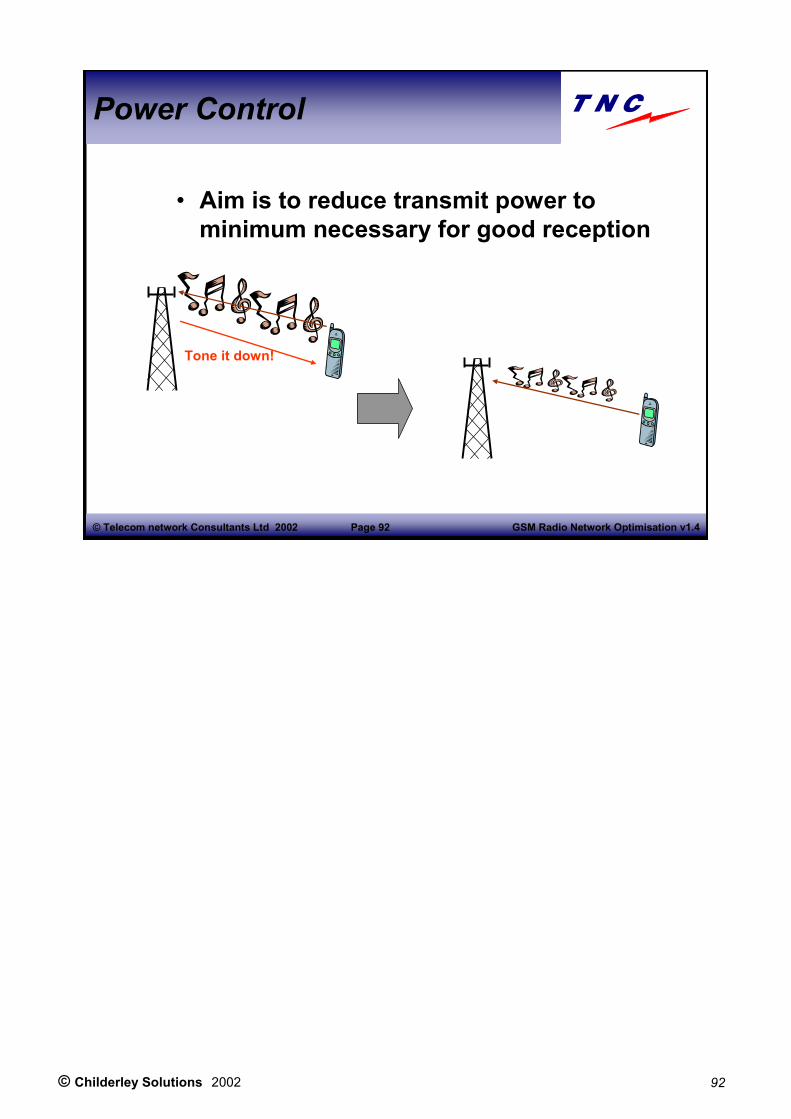
• Aim is to reduce transmit power to minimum necessary for good reception
Tone it down!

© Childerley Solutions 2002 93
GSM Radio Network Optimisation v1.4Page 93© Telecom network Consultants Ltd 2002
Power Control
• Benefits– Reduces interference
• Closer frequency reuse, hence capacity increase
– Minimises battery consumption• Improves talk time of mobiles
– Maximise battery backup consumption• Improves standby time for BTS power supply
– Minimises receiver saturation
© Childerley Solutions 2002 94
GSM Radio Network Optimisation v1.4Page 94© Telecom network Consultants Ltd 2002
Power Control
��MS Power controlMS Power control•• BTS Power controlBTS Power control

© Childerley Solutions 2002 95
GSM Radio Network Optimisation v1.4Page 95© Telecom network Consultants Ltd 2002
MS Power Control
• Possible on TCH & SDCCH– PC on SDCCH enabled by SDCCHREG
– Measured UL signal strength and quality values sent to BSC in Measurement Result message
– Minimum regulation interval between two power control instructions is REGINT
SDCCHREG parameter enables power control
PC command is given every REGINT SACCH period. A new command is sent only if different from previous one.
REGINT cannot be less than one SACCH period (480ms). MS can change power output 8 times in one SACCH period (i.e. every 13th TDMA frame). Power is changed in 2dB steps, giving a total of 16dB change in one SACCH period.
Data Description SourceSignal Strength UL Full set (no DTX) BTSSignal Strength UL Subset (DTX enabled) BTSQuality UL Full set (no DTX) BTSQuality UL Subset (DTX enabled) BTSPower level used by MS MSDTX used by MS or not MS

© Childerley Solutions 2002 96
GSM Radio Network Optimisation v1.4Page 96© Telecom network Consultants Ltd 2002
MS Power Control
• Two modes of operation– Initial regulation: on assignment of new channel and at handover
• MS power reduction only, done very quickly• Short initial signal strength measurement filter
– INILEN measurements needed• No quality input
– Stationary regulation: normal mode• Filter length SSLEN longer than INILEN• Measurements start at same time as initial filter
Initial Regulation: prevents receiver saturation, especially if MS close to BS. Initial regulation performed only after initial filter is filled – and INILEN measurement reports available. Stationary Regulation: will only take place after an initial regulation has been performed.

© Childerley Solutions 2002 97
GSM Radio Network Optimisation v1.4Page 97© Telecom network Consultants Ltd 2002
MS Power Control
• Three process stages– Measurement preparation
• Missing measurements estimated• Selection of full or sub set
– Measurement filtering• Filtering of measurements to remove temporary variations
– Power change calculation• Power step change value calculated, based on received quality. First unconstrained value, then constraints applied.
Measurement filtering: determines if minimum signal strength is received. Quality filtering is average of predetermined number of samples.Power change calculation: two stages, unconstrained, constrained with power step size and MS power range.

© Childerley Solutions 2002 98
GSM Radio Network Optimisation v1.4Page 98© Telecom network Consultants Ltd 2002
MS Power Control
• Measurement preparation– Estimation of some missing measurement
• missing signal value = lowest(value before loss, value after loss).
• missing quality value = worst (value before loss, value after loss).
– Selection of measurement set • Full set used if DTX not enabled• Subset used if DTX enabled
If DTX is not enabled, full set is used, but if DTX is enabled, then subset measurements used. Full set always used for SDCCHMS will continue to use DTX in a new cell when HO occurs, even if new cell does not use DTX. The period of use in new cell is set by DTXFUL.If measurement result missing at next pc command, no extrapolation done for missing signal level and quality measurements, until next set of measurement result received. Then missing signal value = lowest( value before loss, value after loss). missing quality value = worst (value before loss, value after loss).
Estimation of missing MS power level is always done – set to highest known value

© Childerley Solutions 2002 99
GSM Radio Network Optimisation v1.4Page 99© Telecom network Consultants Ltd 2002
MS Power Control
• Measurement Filtering– Signal strength:
• INIDES, target UL value is calculated first
• SScomp=(1/SSLEN)ΣΣΣΣ[SS +MSTXPWR-PWRused)]
– Quality: • QDESUL is the target UL quality• Q_Ave, the filtered rxqual value is average of QLEN samples
• QDESUL and Q_Ave can be transformed into C/I values QDES_dB and Q_Ave_dB
Signal StrengthSScomp: signal strength that would have been received by BTS if no power control is enabled, ie compensated for power reduction regulation. Really is path loss estimation!!SS = actual signal strength received by BTSPWRused = MS output power during measurement periodMSTXPWR = maximum MS output powerSSLEN = filter length (number of samples) for stationary filter.
QualityQuality is measured in rxqual dtqu units (deci-transformed quality units).dtqu = rxqual*10, ranging from dtqu=10 to 100.
Q_Ave_dB and QDES_dB are estimated C/I values, transformed asQ_Ave_dB = 32 – 10*Q_Ave/25Q_DES_dB = 32 – 10*QDESUL/25
Each rxqual = 4 dB

© Childerley Solutions 2002 100
GSM Radio Network Optimisation v1.4Page 100© Telecom network Consultants Ltd 2002
MS Power Control
• Power Order Calculation– Initial phase: unconstrained power order pu
• pu = MSTXPWR – αααα(SScomp –SSDES)– SSDES is target UL signal strength
• “One-shot” stage for achieving the correct power after channel assignment
• No quality parameter involved
LCOMPUL : path loss compensation factor (0-100%), 0=no regulationQCOMPUL: quality deviation compensation factor (0-60%)Normally, PC is a function of signal strength or quality. However, in the Ericsson case, PC function is made to be a combination of both.

© Childerley Solutions 2002 101
GSM Radio Network Optimisation v1.4Page 101© Telecom network Consultants Ltd 2002
MS Power Control
• Power Order Calculation– Stationary phase
• For tracking propagation variations– Includes signal strength and quality parameters
• pu is the absolute power levelpu = MSTXPWR – αααα(SScomp –SSDES) –
ββββ(QDES_dB – Q_Ave_dB)– αααα = LCOMPUL/100 – ββββ = QCOMPUL/100
• dpu is the Power regulation reduction, dpu = LCOMPUL/100*(SScomp –SSDES) –QCOMPUL/100*4/10*(Q_Ave – QDESUL)
LCOMPUL : path loss compensation factor (0-100%), 0=no regulationQCOMPUL: quality deviation compensation factor (0-60%)Normally, PC is a function of signal strength or quality. However, in the Ericsson case, PC function is made to be a combination of both.

© Childerley Solutions 2002 102
GSM Radio Network Optimisation v1.4Page 102© Telecom network Consultants Ltd 2002
MS Power Control
• Example, power order calculation• Let SSDES = -90dBm, SScomp= -64dBm, LCOMPUL=50, QDESUL=10 (rxqual=1) , Q_Ave=40, QCOMPUL=60
Then • Pt1 = 50/100(-64 + 90) = 13 dB • Pt2 = 60/100*4/10*(40-10) = 7.2• dpu = 13 – 7.2 = 5.8 dB power reduction
–– Exercise: How to prevent power reduction Exercise: How to prevent power reduction with poor quality?with poor quality?

© Childerley Solutions 2002 103
GSM Radio Network Optimisation v1.4Page 103© Telecom network Consultants Ltd 2002
MS Power Control
• Power order constraints– constraints are applied if unconstrained power order exceeds dynamic range
• Power step size limitation: 16dB maximum allowable in one SACCH period
• MS Power range: depends on MS power class. Regulation interval ranges from MSTXPWR down to minimum power level of MS

© Childerley Solutions 2002 104
GSM Radio Network Optimisation v1.4Page 104© Telecom network Consultants Ltd 2002
Power Control
•• MS Power controlMS Power control��BTS Power controlBTS Power control

© Childerley Solutions 2002 105
GSM Radio Network Optimisation v1.4Page 105© Telecom network Consultants Ltd 2002
BTS Power Control
• Power order constraints
– Not possible on downlink BCCH carrier– Possible on TCH & SDCCHs
• PC on SDCCH enabled by SDCCHREG• Measured DL signal strength and quality values sent to BSC in Measurement Result message
– Minimum interval between two power control commands is REGINTDL
– Maximum power change is 30dB

© Childerley Solutions 2002 106
GSM Radio Network Optimisation v1.4Page 106© Telecom network Consultants Ltd 2002
BTS Power Control
• Measurement preparation– Output power level conversion– Selection of full or sub data set– Signal strength and quality compensated for use of frequency hopping
• Measurement filtering– Exponential non-linear filters used to eliminate temporary variations

© Childerley Solutions 2002 107
GSM Radio Network Optimisation v1.4Page 107© Telecom network Consultants Ltd 2002
BTS Power Control
• Power Order Calculation: three steps– Calculate two basic power orders pu1, pu2
• BSTXPWR, SSDESDL, SSbstxpwr, QDESDL, Qbstxpwr, αααα1, αααα2, ββββ1, ββββ2, LCOMPDL, QCOMPDL
• pu = max (pu1, pu2) – Apply power order constraints– Convert constrained power order from dBm scale to PLused
• PLused = 0, full power• PLused = 15, 30dB power down
SSDESDL: target value for DL signal strengthQDESDL: target value for DL qualityBSTXPWR:BTS output power on all non BCCH frequencies.BSPWRMIN: minimum allowed BTS output power for non BCCH freqs.SS/Qbstxpwr: signal strength/quality that would be received without use of power control.
If unconstrained power is outside dynamic range, then Power order constraints applied. There are two possible casesIf unconstrained power > BSTXPWR, then pu=BSTXPWRThe lowest pu = max(min BTS output power, BSTXPWR-30, BSPWRMIN)

© Childerley Solutions 2002 108
GSM Radio Network Optimisation v1.4Page 108© Telecom network Consultants Ltd 2002
BTS Power Control
• Power Order Calculation: three steps– Calculate two basic power orders pu1, pu2
• BSTXPWR, • SSDESDL, SSbstxpwr, • QDESDL, Qbstxpwr, • αααα1 = LCOMPDL/100, αααα2 = 0.3• ββββ1 = QCOMPDL/100, ββββ2 = 0.4• pui = ααααi *(SSDESDL - SSbstxpwr) – ββββi *4/10*(Q_Ave –Qbstxpwr)
• pu = max (pu1, pu2) –– Exercise: settings to avoid power reduction on Exercise: settings to avoid power reduction on bad qualitybad quality
SSDESDL: target value for DL signal strengthQDESDL: target value for DL qualityBSTXPWR:BTS output power on all non BCCH frequencies.BSPWRMIN: minimum allowed BTS output power for non BCCH freqs.SS/Qbstxpwr: signal strength/quality that would be received without use of power control.
If unconstrained power is outside dynamic range, then Power order constraints applied. There are two possible casesIf unconstrained power > BSTXPWR, then pu=BSTXPWRThe lowest pu = max(min BTS output power, BSTXPWR-30, BSPWRMIN)

© Childerley Solutions 2002 109
GSM Radio Network Optimisation v1.4Page 109© Telecom network Consultants Ltd 2002
Contents
• BSS Parameters– Idle Mode Behaviour– Measurement Filtering– Power Control– Handover (Locating)

© Childerley Solutions 2002 110
GSM Radio Network Optimisation v1.4Page 110© Telecom network Consultants Ltd 2002
Locating
• Introduction• Ericsson 1• Ericsson 3• Urgency conditions
– Quality– Timing Advance
• Auxiliary functions– Intra-cell handover– Hierarchical cell structures
© Childerley Solutions 2002 111
GSM Radio Network Optimisation v1.4Page 111© Telecom network Consultants Ltd 2002
Locating
• Locating Algorithm– Works out conditions for handover decisions for MS in active mode
– Inputs to algorithm are• Signal strength measurements• Quality measurements
– Output is list of candidate cells for handover• Cells are ranked and sorted in descending order of preference for handover

© Childerley Solutions 2002 112
GSM Radio Network Optimisation v1.4Page 112© Telecom network Consultants Ltd 2002
Locating
• Basic Cell Ranking– Two algorithms
• Ericsson 1: signal strength & path loss• Ericsson 3: signal strength only
– Common process stages• Correction for base station output power
– different levels possible on BCCH/TCH carriers• Calculation of minimum signal strength
– Thresholds MSRXMIN (DL) and BSRXMIN (UL)– SSmin = min (MSRXMIN, BSRXMIN)
• Application of signal strength penalties
What happened to Ericsson 2 ???Algorithms aim to let TCH carriers control cell borders.Corrected signal strength SS_DLn in neighbour cell n: for different output powers between BCCH (BSPWR) and other carriers BSTXPWR:
SS_DLn = rxlevn + BSTXPWRn – BSPWRnMinimum signal strength conditions:
SS_DLn >= MSRXMINnSS_ULn >= BSRXMINn
Where SS_DL is estimated by calculating DL path loss and subtracting from maximum MS output power.
SS_ULn = min(P,MSTXPWRn) – (BSTXPWRn – SS_DLn)Penalties are added to make it more difficult to handover to unsuitable cells. This is done by subtracting a signal value from the signal strength estimate for the unwanted cell, making it look worse than it really is. Penalties are applied for handover failure, bad quality urgency handover and excessive timing advance. A penalty is removed after the penalty duration has expired.

© Childerley Solutions 2002 113
GSM Radio Network Optimisation v1.4Page 113© Telecom network Consultants Ltd 2002
Locating
• Sufficient Level Condition• Threshold separating low signal strength cells from high signal strength cells
high signal strength
low signal strength
DL min levelUL min level
DL effective sufficient level
UL effective sufficient level
B
A
Cells satisfying minimum condition are processed for sufficient condition.
Calculation of sufficient level: s=serving cell, n=neighbour cellSS_DLn >= MSRXSUFFn – TROFFSETn,s + TRHYSTn,sSS_ULn >= BSRXSUFFn – TROFFSETn,s + TRHYSTn,s
Solid lines in diagram represent final combined UL and DL condition. Sufficient level for a serving cell may be different in relation to each different neighbour cell. Setup shown in diagram is valid only for BS pair A,B. It would be different for BS pair A,C.

© Childerley Solutions 2002 114
GSM Radio Network Optimisation v1.4Page 114© Telecom network Consultants Ltd 2002
Locating
• Ranking – signal strength (K) criterion– Signal strength relative to sufficient level
• K-cells = Low signal strength cells, – K values are
– K_DLn,s = SS_DLn,s – MSRXMINn,s– K_ULn,s = SS_ULn,s – BSRXMINn,s
• Effective K value is minimum of UL and DL K values modified by KHYST and KOFFSET
– K ranking• K_RANKn= min(K_DLn, K_ULn) – KOFFSETn,s -KHYSTn,s
• Cells are ranked with the highest K_RANK first
To rank the serving cell as K or L, the sufficient level is evaluated with respect to the best neighbour n1. If K-cell, then it is ranked with the other K-cells. Otherwise, it is ranked with the L-cells.
KHYST is used to decrease ranking values to underrate neighbour cells –to prevent ping pong handovers. Defined for a pair of cells and is always symmetrical KHYSTa,b = KHYSTb,aKOFFSET if positive decreases ranking value and if negative increases ranking value. The cell border is displaced AWAY from cell with positive value, and moved TOWARD the cell with a negative value. It is defined anti-symmetrical for a pair of cells: KOFFSETa,b = -KOFFSETb,a

© Childerley Solutions 2002 115
GSM Radio Network Optimisation v1.4Page 115© Telecom network Consultants Ltd 2002
Locating
• Ranking – path loss (L) criterion– Path loss is assumed symmetrical
• Applied to high signal strength cells – Path Loss values
• p_Ln,s = BSTXPWRn,s – SS_DLn,s
– L ranking values• L_RANKs = p_Ls• L_RANKn = p_Ln + LOFFSETn,s + LHYSTn,s• Cells are ranked with the lowest L_RANK first
LHYST and LOFFSET have the same properties as the K counterparts.
Path Loss criterion is independent of BS and MS power ratings. It facilitates transfer of calls from big cell (strong interference) to small cells (less interference). L-criterion should lower overall statistical interference in network

© Childerley Solutions 2002 116
GSM Radio Network Optimisation v1.4Page 116© Telecom network Consultants Ltd 2002
Locating
• Basic Ranking Candidate List
L-cells list
K-cells list
Best cell
Worst cell
Highest L-Rank (lowest path loss)
Lowest L-Rank
Highest K-Rank (highest signal level)
Lowest K-Rank
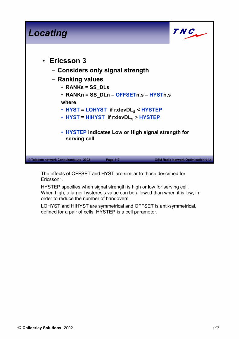
© Childerley Solutions 2002 117
GSM Radio Network Optimisation v1.4Page 117© Telecom network Consultants Ltd 2002
Locating
• Ericsson 3– Considers only signal strength– Ranking values
• RANKs = SS_DLs• RANKn = SS_DLn – OFFSETn,s – HYSTn,swhere• HYST = LOHYST if rxlevDLS < HYSTEP• HYST = HIHYST if rxlevDLS ≥≥≥≥ HYSTEP
• HYSTEP indicates Low or High signal strength for serving cell
The effects of OFFSET and HYST are similar to those described for Ericsson1. HYSTEP specifies when signal strength is high or low for serving cell. When high, a larger hysteresis value can be allowed than when it is low, in order to reduce the number of handovers. LOHYST and HIHYST are symmetrical and OFFSET is anti-symmetrical, defined for a pair of cells. HYSTEP is a cell parameter.

© Childerley Solutions 2002 118
GSM Radio Network Optimisation v1.4Page 118© Telecom network Consultants Ltd 2002
Locating
• Urgency Condition: Bad Quality– Handover is initiated when rxqual exceeds specified thresholds, even if the level is good
• rxqualUL > QLIMUL or • rxqualDL > QLIMDL
– Handover is allowed to cell of lower ranking, but not to cell with worse quality.
• BQOFFSET, applied to K-rank and L-rank values, defines how far from nominal border MS can be to qualify for the quality handover.
When BQ urgency exists, unsuitable neighbours are removed from candidate list. Signal strength of serving cell is compared with signal strength of candidates, and those cells with large differences are removed from the list.Ericsson1If K_RANKn – K_RANKs < -KHYSTn,s – BQOFFSETn,s remove n.If L_RANKn – L_RANKs > LHYSTn,s – BQOFFSETn,s remove n.Ericsson3If RANKn – RANKs < -HYSTn,s – BQOFFSETn,s remove n.
If BQ urgency handover performed, a penalty value PSSBQ and penalty duration PTIMBQ are applied to prevent immediate handover back to the old cell.
AB
Hysteresis corridor BQ urgency HO prohibited
BQ urgency region
BQOFFSETb,aNominal cell border

© Childerley Solutions 2002 119
GSM Radio Network Optimisation v1.4Page 119© Telecom network Consultants Ltd 2002
Locating
• Urgency Condition: Timing Advance– Timing advance (TA) can be used as a soft cell limiter, to force small cells
– TALIM is the defined cell limit, maximum (63 bits or 35 km).
– TA urgency occurs if TAs ≥≥≥≥ TALIM – Urgent handover is performed to neighbour cells where TAn < TALIMs
– If no suitable candidate found, call remains on serving cell
If TA urgency handover performed, a penalty value PSSTA and penalty duration PTIMTA is applied to prevent immediate handover back to the old cell.
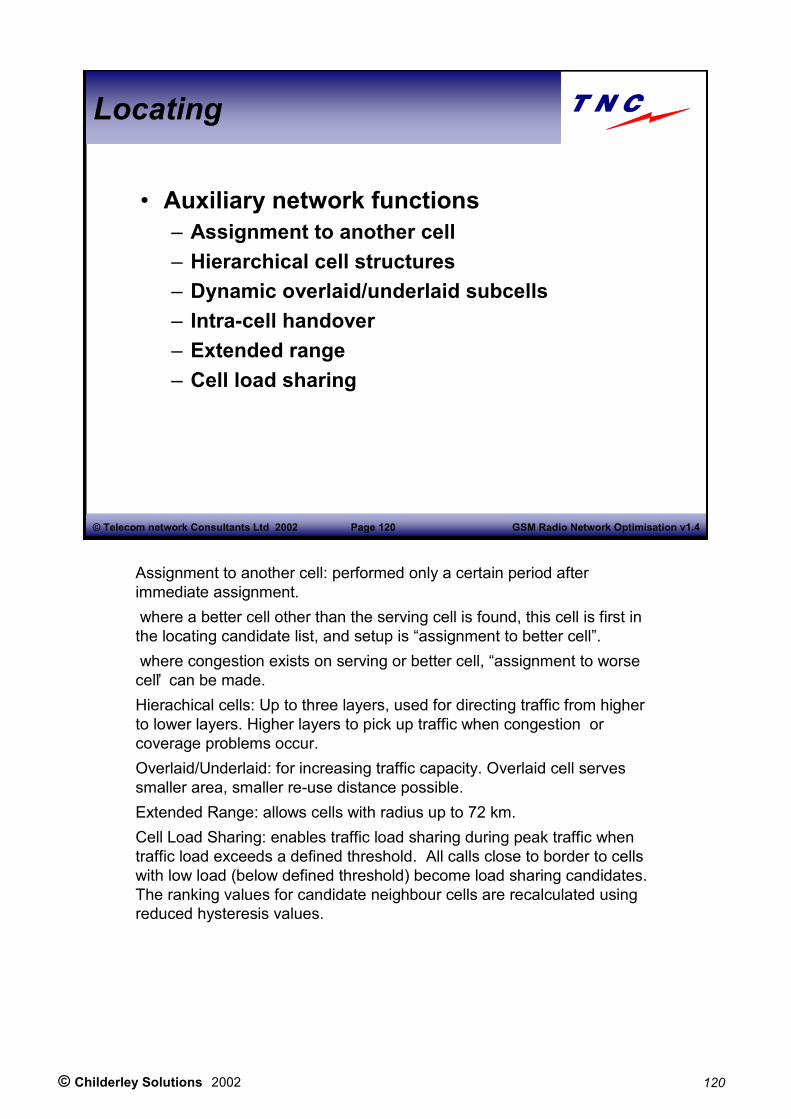
© Childerley Solutions 2002 120
GSM Radio Network Optimisation v1.4Page 120© Telecom network Consultants Ltd 2002
Locating
• Auxiliary network functions – Assignment to another cell– Hierarchical cell structures– Dynamic overlaid/underlaid subcells– Intra-cell handover– Extended range– Cell load sharing
Assignment to another cell: performed only a certain period after immediate assignment.where a better cell other than the serving cell is found, this cell is first in
the locating candidate list, and setup is “assignment to better cell”.where congestion exists on serving or better cell, “assignment to worse
cell” can be made.Hierachical cells: Up to three layers, used for directing traffic from higher to lower layers. Higher layers to pick up traffic when congestion or coverage problems occur.Overlaid/Underlaid: for increasing traffic capacity. Overlaid cell serves smaller area, smaller re-use distance possible.Extended Range: allows cells with radius up to 72 km.Cell Load Sharing: enables traffic load sharing during peak traffic when traffic load exceeds a defined threshold. All calls close to border to cells with low load (below defined threshold) become load sharing candidates. The ranking values for candidate neighbour cells are recalculated using reduced hysteresis values.

© Childerley Solutions 2002 121
GSM Radio Network Optimisation v1.4Page 121© Telecom network Consultants Ltd 2002
Locating
• Intra-cell handover– Try to find another frequency and/or timeslot in the same cell with better quality
– Only if RxQual is bad AND RxLev is good• RxQual_UL/DL > QOFFSETUL/DL +FQSS(RXLEV_UL/DL +SSOFSETUL/DL)
– RxLev_DL/UL = actual measured signal strengths, no pc compensation
– FQSS = quality vs signal strength function– Does not work for:
• BCCH downlink• Random frequency hopping
QOFFSETUL/DL: quality offset parameters uplink/downlinkSSOFSETUL/DL: signal strength offset parameters uplink/downlinkFQSS table
RXLEV rxqual<=30 infinity31 6032-35 5936-38 5839-41 5742-45 5646-48 5549-52 5453-55 5356-58 5259-62 51>=63 50
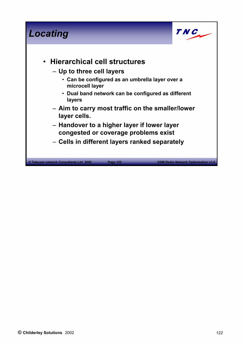
© Childerley Solutions 2002 122
GSM Radio Network Optimisation v1.4Page 122© Telecom network Consultants Ltd 2002
Locating
• Hierarchical cell structures– Up to three cell layers
• Can be configured as an umbrella layer over a microcell layer
• Dual band network can be configured as different layers
– Aim to carry most traffic on the smaller/lower layer cells.
– Handover to a higher layer if lower layer congested or coverage problems exist
– Cells in different layers ranked separately

© Childerley Solutions 2002 123
GSM Radio Network Optimisation v1.4Page 123© Telecom network Consultants Ltd 2002
BSS Parameters - review
• Idle mode behaviour• Measurement filtering• Power Control• Handover (Locating)

© Childerley Solutions 2002 124
GSM Radio Network Optimisation v1.4Page 124© Telecom network Consultants Ltd 2002
Contents
• System Basics• BSS Parameters�Quality Assessment• Optimisation Measures• Organisation

© Childerley Solutions 2002 125
GSM Radio Network Optimisation v1.4Page 125© Telecom network Consultants Ltd 2002
Contents
• Quality Assessment�Network Performance Measurements
• Use of statistics• Traffic• Blocking• Dropped calls• Noisy calls• Call success rate• Handover causes
– Field Measurements

© Childerley Solutions 2002 126
GSM Radio Network Optimisation v1.4Page 126© Telecom network Consultants Ltd 2002
Network performance stats
• Use of statistics• Traffic• Blocking• Dropped calls• Noisy calls• Call success rate• Handover causes

© Childerley Solutions 2002 127
GSM Radio Network Optimisation v1.4Page 127© Telecom network Consultants Ltd 2002
Network Performance Stats
• Introduction– Counters are available from the OMC, eg:
• Traffic volume• Blocking rates• RxQual• RxLev• Handover success• Dropped calls… etc etc….
– Evaluated by cell, BSC, MSC etc– Software is available to process counters
This is a very good source of information given that the amount of traffic in the network is high enough to provide reliable statistics. In order to facilitate the identification and resolution of problems, it is important to determine the key system metrics to monitor. The frequency and level of detail of the report should also be set to ensure that there is sufficient information for the groups involved in the optimisation activities, and for management. Important key metrics which should be considered include call success rate, blocking (TCH and SDCCH), call setup and handover success. The performance monitoring tool will produce regular statistics reports for each cell for the previous 24 hours. The metrics will be calculated for the busy hour for each cell. Different operators offer different counters. E.g. some count number of RxQual=5, others count noisy calls, or noisy call minutes.

© Childerley Solutions 2002 128
GSM Radio Network Optimisation v1.4Page 128© Telecom network Consultants Ltd 2002
Network Performance Stats
• Types of thresholds
– Target• Desired/specified threhold
– Optimisation• Level at which improvement is required
– Fault• Level indicating serious problem requiring immediate rectification
The key performance parameters are monitored against a set of thresholds: Target, optimisation and fault thresholdsThe Target threshold is defined as the level that enables the customer to initiate and complete a call successfully with good quality. The Optimisation threshold is defined as the level for a performance indicator which requires some improvement. This threshold will focus attention on the worst performing cells and optimisation activities are scheduled along with any others and implemented as necessary. The Fault threshold is defined as the level for a performance indicator which represents a serious problem and is considered to be a fault condition. It therefore requires an immediate solution and the necessary optimisation activities should be scheduled with greater priority.
The thresholds may change depending on the maturity of the network, and should be periodically reviewed.

© Childerley Solutions 2002 129
GSM Radio Network Optimisation v1.4Page 129© Telecom network Consultants Ltd 2002
Network Performance StatsMetric Definition Target
thresholdOptimisati
on threshold
Fault threshold
Comments
Call attempts Number attempts to start a speech, dat or fax call.
400 for signifi canc
e
N/A N/A Used to evaluate the significance of other metrics
Setup success rate Number o f successful TCH call setups out of call attempts.
96% 92% 80%
Call completion suc cess rate
Calls which, once set upare successfully con cluded
98% 92% 80%
Dropped call rate 1 - Call completion suc cess rate
2% 8% 20%
TCH RF- loss rate % Calls dropped only due to interference or lack of signal (Radio Link Timeout and handover timeout)
2% 8% 20% Pointer to coverage holes, or to interference caused by a bad frequency plan, or to an RxLe vAccessMin which is too low, or RTL too short.
SDCCH RF- loss rate %SD CCH channels dropped only due to inter ference or lack of signal
2% 8% 20% Pointer to coverage holes, or to interference caused by a bad frequency plan or to an RxLe vAccessMin which is too low. Also includes failed LAC up dates.
TCH blocking rate Failed TC H assignments because all TCHs are in use.
1% 2% 20% An indication of whether there are sufficient transceivers on the cell. Normally the network should have been extended to cope with traffic growth before blocking is experi enced.
SDCCH blocking rate Fa iled SDCCH assignmentsbecause all TCHs are in use.
0.5% 1% 5%
Intra cell HO success rate Handovers between timeslots on the same cell
96% 90% 80%
Inter cell HO success rate 96% 90% 80%
TCH traffic Busy hour traffic in Er langs, average of the 5 daily busiest hours in the last week.
N/A N/A N/A Used to weight the metrics and to plan growth. (See traffic planning
guidelines).
Metr ic Definition Target thres h old
Optimis a tion
threshold
Fault thres h old
Comments
Call attempts Number attempts to start a speech, dat or fax call.
400 for signif i canc
e
N/A N/A Used to evaluate the significance of other metrics
Setup success rate Number o f successful TCH call setups out of call
attempts.
96% 92% 80%
Call completion su c cess rate
Calls which, once set upare successfully co n cluded
98% 92% 80%
Dropped call rate 1 - Call completion su c cess rate
2% 8% 20%
TCH RF - loss rate % Calls dropped only due to interference or lack of signal (Radio Link Timeout
and handover tim e out)
2% 8% 20% Pointer to coverage holes, or to interference caused by a bad frequency plan, or to an
RxLe vAccessMin which is too low, or RTL too short.
SDCCH RF - loss rate %SD CCH channels dropped only due to
inte r ference or lack of signal
2% 8% 20% Pointer to coverage holes, or to interference caused by a bad frequency plan or to an
RxLe vAccessMin which is too low. Also includes failed LAC u p dates.
TCH blocking rate Failed TC H assignments because all TCHs are in use.
1% 2% 20% An indication of whether there are sufficient transceivers on the cell. Normally the network should have been extended to cope with traffic growth before blocking is
exper i enced.
SDCCH blocking rate Fa iled SDCCH assig n mentsbecause all TCHs are in use.
0.5% 1% 5%
Intra cell HO success rate Handovers between timeslots on the same cell
96% 90% 80%
Inter cell HO success rate 96% 90% 80%
TCH traffic Busy hour traffic in E r langs, average of the 5 dail y busiest hours in the last
week.
N/A N/A N/A Used to weight the metrics and to plan growth. (See traffic planning
guidelines).

© Childerley Solutions 2002 130
GSM Radio Network Optimisation v1.4Page 130© Telecom network Consultants Ltd 2002
Network Performance Stats
• Significance of statistics– Binominal distribution
• Ask 10 people if they are married• 5 say yes• Are 50% of all people married?• 45% to 55%?• Chance that 40% or 60% are married.
To have a resolution of 1% in the call success rate would require 100 samples. However, there is still a distribution of the measured results around the true probability.

© Childerley Solutions 2002 131
GSM Radio Network Optimisation v1.4Page 131© Telecom network Consultants Ltd 2002
Network Performance Stats
• Significance of statistics– Binominal distribution
Confidence of 1% accuracy for given number of calls
0.0%
10.0%
20.0%
30.0%
40.0%
50.0%
60.0%
70.0%
80.0%
90.0%
100.0%
0 100 200 300 400 500 600 700 800 900 1000 1100 1200Number of Calls
Con
fidence Probability
2%
5%
10%
20%
Dropped call rate
Confidence of 1% accuracy for given number of calls
0.0%
10.0%
20.0%
30.0%
40.0%
50.0%
60.0%
70.0%
80.0%
90.0%
100.0%
0 100 200 300 400 500 600 700 800 900 1000 1100 1200Number of Calls
Confid
ence Probability
2%
5%
10%
20%
Dropped call rate

© Childerley Solutions 2002 132
GSM Radio Network Optimisation v1.4Page 132© Telecom network Consultants Ltd 2002
Network Performance Stats
• Significance of statistics
– Hundreds of samples must be taken to be 90% confident of only a ±1% tolerance
– Combine Busy hour statistics for the whole week

© Childerley Solutions 2002 133
GSM Radio Network Optimisation v1.4Page 133© Telecom network Consultants Ltd 2002
Network Performance Stats
• Traffic– Traffic volume must include time period
– Busy hour normally• eg 3 busiest hrs of the week
– First work out when is the busy hour• Requires all-day measurements
– TCH traffic and SDCCH traffic
– Busy hour important for ALL statistics
The determination of the busy hour is important for all statistics. Many problems only manifest when load is high. Exception: downlink BCCH interference.

© Childerley Solutions 2002 134
GSM Radio Network Optimisation v1.4Page 134© Telecom network Consultants Ltd 2002
Network Performance Stats
• Traffic– Forecasting– Weekly busy hour traffic extrapolated
Traffic
Time
Individual cells can have forecast traffic growth estimated before the traffic is combined into a traffic map.

© Childerley Solutions 2002 135
GSM Radio Network Optimisation v1.4Page 135© Telecom network Consultants Ltd 2002
Network Performance Stats
• Traffic– Forecasting– Local growth or national growth?
Traffic
Time
Individual cells might have a significantly different prognosis than the overall growth forecast. For example a high traffic cell might cover the operator’s headquarters. Fast early growth, but now saturated.

© Childerley Solutions 2002 136
GSM Radio Network Optimisation v1.4Page 136© Telecom network Consultants Ltd 2002
Network Performance Stats
• Traffic– Forecast 3 months ahead for TRX count
• Procurement• Frequency planning
– Forecast 12 months ahead for site count• Planning • Acquisition• Build
The frequency planning of the next turn-on-cycle will require as an input the amount of traffic in each cell. The cell capacity will need to last until the turn-on-cycle after that. A margin for error must be included.

© Childerley Solutions 2002 137
GSM Radio Network Optimisation v1.4Page 137© Telecom network Consultants Ltd 2002
Network Performance Stats
• Blocking rate– Must be measured in the BH
• Traffic measurements required first• TCH blocking and SDCCH blocking
– Need to know:• Number of Call Attempts• Number of Successful TCH (or SDCCH) seizures
– Utilisation• % of TCH in use
In a frequency hopping system it may be that hard blocking does not occur, only soft blocking.

© Childerley Solutions 2002 138
GSM Radio Network Optimisation v1.4Page 138© Telecom network Consultants Ltd 2002
Network Performance Stats
• Dropped calls– Various causes for this:
• Poor BER (Radio Link Timeout – RF Loss)• Deliberate disconnection (eg maximum range)• Hardware problems• Fixed network problems
• Lots of obscure counters!

© Childerley Solutions 2002 139
GSM Radio Network Optimisation v1.4Page 139© Telecom network Consultants Ltd 2002
Network Performance Stats
• Noisy calls– RxQual measurements
• What is the definition of a noisy call?– e.g. 10% of RxQual ≥≥≥≥ 4
• Classify individual calls within the cell to identify problem cells
• Alternatively, determine by using all RxQual measurements taken over a measurement period (uplink and downlink)

© Childerley Solutions 2002 140
GSM Radio Network Optimisation v1.4Page 140© Telecom network Consultants Ltd 2002
Network Performance Stats
• Call success rate– Service (coverage)– No blocking– No RF Loss or other drop– Not defined as noisy
– From the network it is not possible to see call attempts which fail due to no coverage.

© Childerley Solutions 2002 141
GSM Radio Network Optimisation v1.4Page 141© Telecom network Consultants Ltd 2002
Network Performance Stats
• Call success rate– Target for a new (or newly expanded) network:
90% for each cell95% for each BSC
– Target for a mature network:96% for each cell98% for each BSC
The target performance of course needs to be met in the busy hour. Averaging over the whole day is cheating!

© Childerley Solutions 2002 142
GSM Radio Network Optimisation v1.4Page 142© Telecom network Consultants Ltd 2002
Network Performance Stats
• Call success rate– Report to the responsible engineer on a weekly basis:
• Any cells in engineer’s area not meeting the target • Or the 10 worst cells in engineer’s area
• (First remove cells whose poor performance is due to a known hardware problem)

© Childerley Solutions 2002 143
GSM Radio Network Optimisation v1.4Page 143© Telecom network Consultants Ltd 2002
Network Performance Stats
• Handover causes– Power Budget (L-criterion) should be dominant (90%)
– Signal level (K-criterion) only for indoors
– Quality cause should be rare
– Distance cause only in rural areas
– Uplink and Downlink causes

© Childerley Solutions 2002 144
GSM Radio Network Optimisation v1.4Page 144© Telecom network Consultants Ltd 2002
Network Performance Stats
• Link balance– Imbalance in statistics (eg noisier uplink than downlink) can be caused by link imbalance
• Can carry out detailed measurements of cables, combiners, output powers, sensitivities, diversity gains, etc
• Can analyse NPC data or A-bis traces.
The A-bis interface is between the BS and the BSC. Possible to record all RxQual measurements for the cell in uplink and downlink. Imprt these into Excel and perform regression analysis.

© Childerley Solutions 2002 145
GSM Radio Network Optimisation v1.4Page 145© Telecom network Consultants Ltd 2002
Network performance review
• Use of statistics• Traffic• Blocking• Dropped calls• Noisy calls• Call success rate• Handover causes

© Childerley Solutions 2002 146
GSM Radio Network Optimisation v1.4Page 146© Telecom network Consultants Ltd 2002
Contents
• Quality Assessment– Network Performance Measurements �Field Measurements
�Measurement Equipment�Statistics�Analysis�Call Logging Equipment

© Childerley Solutions 2002 147
GSM Radio Network Optimisation v1.4Page 147© Telecom network Consultants Ltd 2002
Field measurements
• Measurement kit• Statistics• Analysis• Call logging equipment
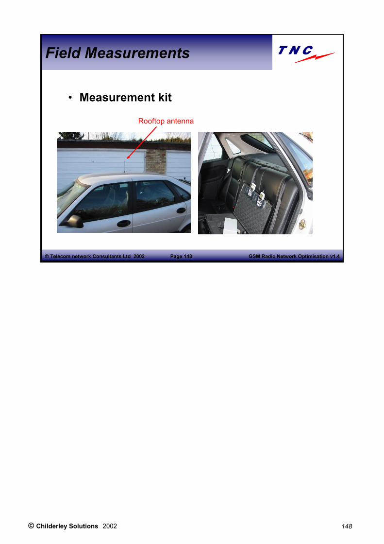
© Childerley Solutions 2002 148
GSM Radio Network Optimisation v1.4Page 148© Telecom network Consultants Ltd 2002
Field Measurements
• Measurement kit
Rooftop antenna

© Childerley Solutions 2002 149
GSM Radio Network Optimisation v1.4Page 149© Telecom network Consultants Ltd 2002
Field Measurements
• Measurement kit– Engineering enabled mobile
• Records downlink measurements every 480 ms in dedicated mode
• Serving cell: – BCCH, BSIC, RxLev, RxQual, TA– Layer three messages
• Neighbour cells– BCCH, BSIC, RxLev_N
– GPS receiver• Location of every measurement• Enables display on a map
Engineering mobiles manufactured by SAGEM, Ericsson, Nokia etc. These mobiles have special engineering software (not available to Joe Bloggs on the street) that is used for measuring the relevant data. They do not have storage capabilities, therefore, data collected must be stored elsewhere. Known test mobiles include:• Nokia: 8148, PT11• Ericsson: TEMS pocket• SAGEM: OT35• Nortel: 1822

© Childerley Solutions 2002 150
GSM Radio Network Optimisation v1.4Page 150© Telecom network Consultants Ltd 2002
Field Measurements
• Statistics– Call success rate– Probability of coverage
• Signal above required threshold, NOT above median planning level
• Check “indoor coverage” with a 20 dB attenuator– post processing RxLevs would have to take into account DL power control

© Childerley Solutions 2002 151
GSM Radio Network Optimisation v1.4Page 151© Telecom network Consultants Ltd 2002
Field Measurements
• Data analysis– Dropped calls– In-building Coverage
RxLev > -90 dBm– (= -102 + 18 – 6 = -90dBm)

© Childerley Solutions 2002 152
GSM Radio Network Optimisation v1.4Page 152© Telecom network Consultants Ltd 2002
Field Measurements
• RxQual– Acceptable <= 4– Unacceptable >= 5

© Childerley Solutions 2002 153
GSM Radio Network Optimisation v1.4Page 153© Telecom network Consultants Ltd 2002
Field Measurements
• Outdoor coverage– RxLev ≥≥≥≥ -108 dBm– (-102 - 6 dB = -108 dBm)

© Childerley Solutions 2002 154
GSM Radio Network Optimisation v1.4Page 154© Telecom network Consultants Ltd 2002
Field Measurements

© Childerley Solutions 2002 155
GSM Radio Network Optimisation v1.4Page 155© Telecom network Consultants Ltd 2002
Field Measurements
• Dropped call - interference
In this example the signal level is reasonably good, while the RxQual is bad, indicating an area of interference led to the call dropping.

© Childerley Solutions 2002 156
GSM Radio Network Optimisation v1.4Page 156© Telecom network Consultants Ltd 2002
Field Measurements
• Dropped call - coverage
The serving signal drops very low, and the signals from neighbouring cells are also low, so there is no opportunity for a handover. In the low signal, the BER becomes high and the call drops.

© Childerley Solutions 2002 157
GSM Radio Network Optimisation v1.4Page 157© Telecom network Consultants Ltd 2002
Field Measurements
• Dropped Call - Unexpected release
In this example the signal level is adequate, and the BER remains low. Nevertheless the call is terminated by a network command.

© Childerley Solutions 2002 158
GSM Radio Network Optimisation v1.4Page 158© Telecom network Consultants Ltd 2002
Field Measurements
The Layer 3 messages indicate that the call dropped because there were no channels available on the target cell during a handover. The mobile fell back to the original cell, which eventually became unusable
.

© Childerley Solutions 2002 159
GSM Radio Network Optimisation v1.4Page 159© Telecom network Consultants Ltd 2002
Field Measurements
• Call logging equipment
– Test mobile (eg TEMS) in taxis, buses and employees cars, making repeated calls
• 2 minute call every 2.5 minutes• Data deleted if call is successful• If call drops within two minutes, call into computer via modem and download data for analysis
• Statistical results including no service areas
This method of data collection is sometimes used to collect data, in addition to regular drive testing, or when the network needs to be “ loaded”for specific investigation. It requires finding friendly customers that will agree to having the equipment installed in their vehicles for long periods of time. It is quite subjective in that the measurement routes are defined by the daily routine of the vehicle in which the kit is installed. However, it is highly likely that the calls will be made where there is potential “people traffic”.

© Childerley Solutions 2002 160
GSM Radio Network Optimisation v1.4Page 160© Telecom network Consultants Ltd 2002
Field measurements - review
• Measurement kit• Analysis• Statistics• Call logging equipment

© Childerley Solutions 2002 161
GSM Radio Network Optimisation v1.4Page 161© Telecom network Consultants Ltd 2002
Contents
• System Basics• BSS Parameters• Quality Assessment�Optimisation Measures• Organisation

© Childerley Solutions 2002 162
GSM Radio Network Optimisation v1.4Page 162© Telecom network Consultants Ltd 2002
Contents
• Optimisation Measures�Antenna Adjustments– Frequency & Interference Planning– Neighbour List Planning– Common Problems– Advanced Techniques

© Childerley Solutions 2002 163
GSM Radio Network Optimisation v1.4Page 163© Telecom network Consultants Ltd 2002
Antenna adjustments
• Tilt• Electrical and mechanical tilt• Side-lobes and nulls
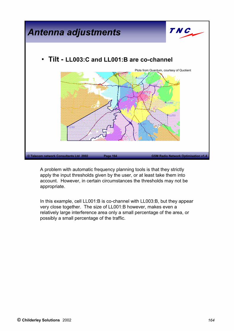
© Childerley Solutions 2002 164
GSM Radio Network Optimisation v1.4Page 164© Telecom network Consultants Ltd 2002
Antenna adjustments
• Tilt - LL003:C and LL001:B are co-channelPlots from Quantum, courtesy of Quotient
A problem with automatic frequency planning tools is that they strictly apply the input thresholds given by the user, or at least take them into account. However, in certain circumstances the thresholds may not be appropriate.
In this example, cell LL001:B is co-channel with LL003:B, but they appear very close together. The size of LL001:B however, makes even a relatively large interference area only a small percentage of the area, or possibly a small percentage of the traffic.

© Childerley Solutions 2002 165
GSM Radio Network Optimisation v1.4Page 165© Telecom network Consultants Ltd 2002
Antenna adjustments
• Tilt -AFP tolerates interference (<10% of traffic?)Plots from Quantum, courtesy of Quotient
In this case a relatively large area of interference only affects a small number of Erlangs. However the area affected is a short stretch of very important road. In addition, the prediction radius for LL003 does not appear to be large enough. Other interference exists, which is not shown on the plot.
The network needs to be optimised to remove this interference in the BCCH layer.
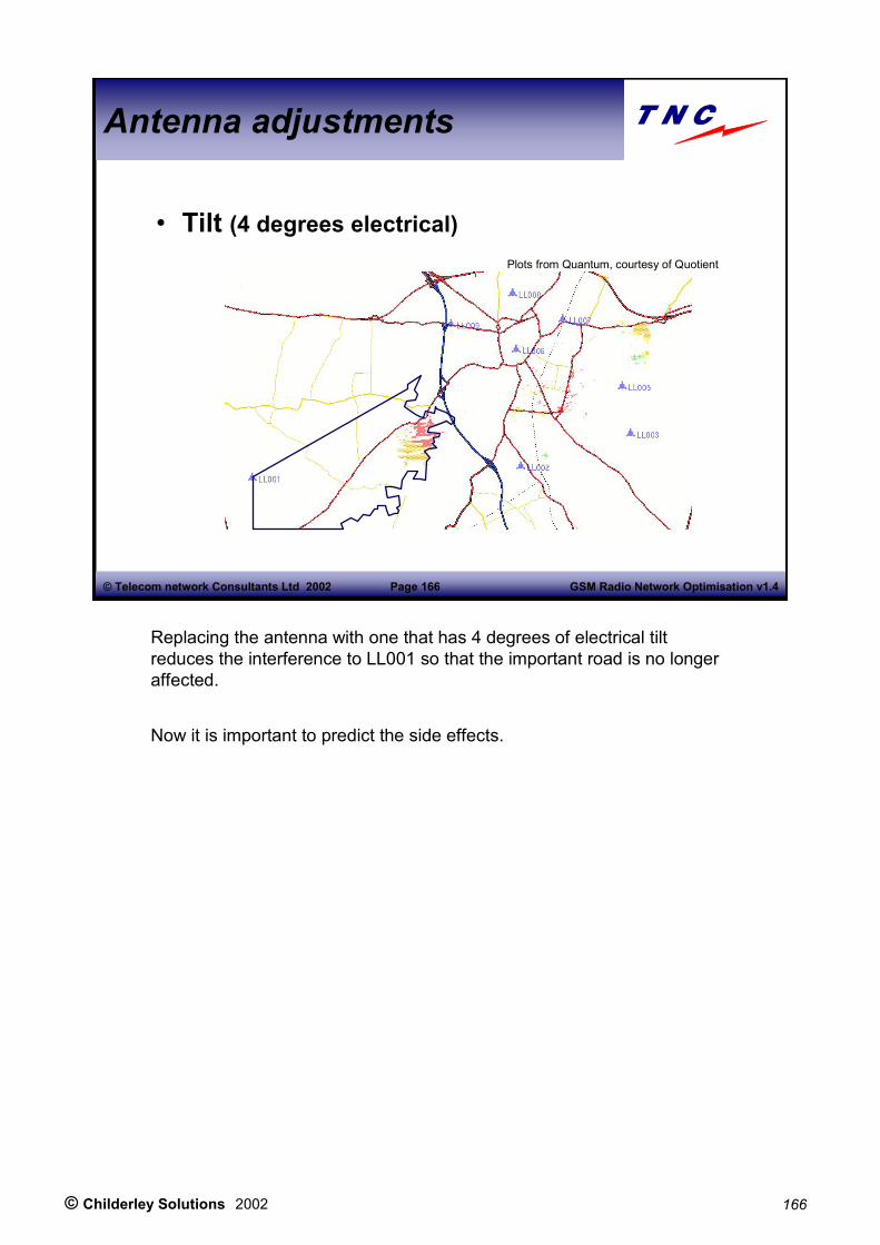
© Childerley Solutions 2002 166
GSM Radio Network Optimisation v1.4Page 166© Telecom network Consultants Ltd 2002
Antenna adjustments
• Tilt (4 degrees electrical)Plots from Quantum, courtesy of Quotient
Replacing the antenna with one that has 4 degrees of electrical tilt reduces the interference to LL001 so that the important road is no longer affected.
Now it is important to predict the side effects.

© Childerley Solutions 2002 167
GSM Radio Network Optimisation v1.4Page 167© Telecom network Consultants Ltd 2002
Antenna adjustments
• Tilt (4 degrees electrical)– Check side effects
Coverage compromised?
Plots from Quantum, courtesy of Quotient
Tilting the beam has reduced the interference, but has also reduced the signal level closer to the site and a couple of coverage holes have appeared.Can the other road tolerate a lower signal in order to give the first road interference free coverage?Maybe a 2 degree tilt would have been sufficient?Perhaps a combination of tilt and a change in azimuth a few degrees to the south would give both roads good quality.A better solution might have been to substitute a new BCCH frequency in either of the two cells. However this might just move the interference to somewhere else.
It is the cell planner / optimiser who must make the decisions regarding the trade offs. This is why it is better that optimisers and cell planners are the same people.

© Childerley Solutions 2002 168
GSM Radio Network Optimisation v1.4Page 168© Telecom network Consultants Ltd 2002
Antenna adjustments
• Sidelobes– In the vertical pattern of most antennas are sidelobes
• Too much tilt can start to increase interference again
• Nulls– The null in the vertical pattern is best pointed towards the horizon
– Nulls below the horizontal can cause coverage holes close to the site

© Childerley Solutions 2002 169
GSM Radio Network Optimisation v1.4Page 169© Telecom network Consultants Ltd 2002
Antenna adjustments - review
• Tilt• Electrical and mechanical tilt• Side-lobes and nulls
© Childerley Solutions 2002 170
GSM Radio Network Optimisation v1.4Page 170© Telecom network Consultants Ltd 2002
Contents
• Optimisation Measures– Antenna Adjustments�Frequency & Interference Planning– Neighbour List Planning– Common Problems– Advanced Techniques

© Childerley Solutions 2002 171
GSM Radio Network Optimisation v1.4Page 171© Telecom network Consultants Ltd 2002
Frequency planning
• Cell planning practice• BCCH carrier planning and optimisation• Non-BCCH carriers• Frequency hopping• Interference reduction
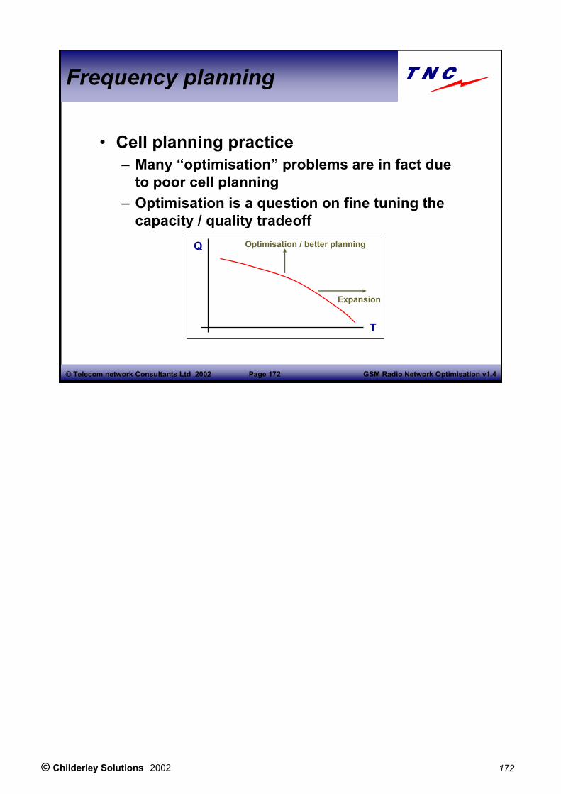
© Childerley Solutions 2002 172
GSM Radio Network Optimisation v1.4Page 172© Telecom network Consultants Ltd 2002
Frequency planning
• Cell planning practice– Many “optimisation” problems are in fact due to poor cell planning
– Optimisation is a question on fine tuning the capacity / quality tradeoff
Q
T
Expansion
Optimisation / better planning

© Childerley Solutions 2002 173
GSM Radio Network Optimisation v1.4Page 173© Telecom network Consultants Ltd 2002
Frequency planning
• Cell planning practice– Problems when
• Interference not contained• One cell carries too much traffic• Inappropriate position of cell boundaries• Multiple servers• Imprecise service area
– All the above will affect the quality for a given traffic load (or the traffic load for a given quality)
• by making frequency planning harder
© Childerley Solutions 2002 174
GSM Radio Network Optimisation v1.4Page 174© Telecom network Consultants Ltd 2002
Frequency planning
• BCCH carrier planning– For BCCH carriers downlink interference always present
– Frequency plan must be interference free– Interference can be removed by changing the frequency plan
© Childerley Solutions 2002 175
GSM Radio Network Optimisation v1.4Page 175© Telecom network Consultants Ltd 2002
Frequency planning
• Non-BCCH carriers– Interference affected by DTX, PC and load
– PC more effective if most traffic is near the site
– Frequency planning relatively easy (1/3 or 1/1)
– Main issue is traffic planning

© Childerley Solutions 2002 176
GSM Radio Network Optimisation v1.4Page 176© Telecom network Consultants Ltd 2002
Frequency planning
• Frequency hopping– With 1/3 or 1/1, and fractional load: swapping frequencies does not remove interference
– Important to limit interference for all cells– New site? Surrounding cells should all have down-tilts reviewed.

© Childerley Solutions 2002 177
GSM Radio Network Optimisation v1.4Page 177© Telecom network Consultants Ltd 2002
Frequency planning
• Interference reduction– Antenna tilt– Reduced height – Reduced power– Terrain or clutter containment

© Childerley Solutions 2002 178
GSM Radio Network Optimisation v1.4Page 178© Telecom network Consultants Ltd 2002
Frequency planning - review
• Cell planning practice• BCCH carrier planning and optimisation• Non-BCCH carriers• Frequency hopping• Interference reduction

© Childerley Solutions 2002 179
GSM Radio Network Optimisation v1.4Page 179© Telecom network Consultants Ltd 2002
Contents
• Optimisation Measures– Antenna Adjustments– Frequency & Interference Planning�Neighbour List Planning– Common Problems– Advanced Techniques

© Childerley Solutions 2002 180
GSM Radio Network Optimisation v1.4Page 180© Telecom network Consultants Ltd 2002
Neighbour list planning
• Too many neighbours• Too few neighbours• Automatic neighbour planning• Undefined neighbour reporting• Double BA lists

© Childerley Solutions 2002 181
GSM Radio Network Optimisation v1.4Page 181© Telecom network Consultants Ltd 2002
Neighbour lists
• Too many neighbours– Impossible adjacent channel planning– Co-channel planning made difficult– Inappropriate handovers to distant cells– Less accurate neighbour RxLev measurements
Update neighbour lists in cells surrounding a new site!
The time for neighbour measurements is fixed within the SACCH multiframe. More neighbours means fewer samples are taken of each neighbour’s signal level. There is an opportunity for measurement once every TDMA frame, so 104 measurements every 480 ms.
For example, 6 neighbours : 17 samples per neighbour per measurement report. 26 neighbours is only 4 samples per neighbour per measurement report.

© Childerley Solutions 2002 182
GSM Radio Network Optimisation v1.4Page 182© Telecom network Consultants Ltd 2002
Neighbour lists
• Too few neighbours– No handover– Idle mode problems when returning to coverage
The problems of missing neighbours are obvious. Perhaps for this reason most networks seem to have too many neighbour relationships.

© Childerley Solutions 2002 183
GSM Radio Network Optimisation v1.4Page 183© Telecom network Consultants Ltd 2002
Neighbour lists
• Automatic neighbour planning– Measure length of common boundary– Determine area of overlap
• Overlap defined as where 2nd (or nth) server is less than X dB below the best server
– Second method preferred
– Manual fine tuning normally necessary: not too bad in a mature network
© Childerley Solutions 2002 184
GSM Radio Network Optimisation v1.4Page 184© Telecom network Consultants Ltd 2002
Neighbour lists
• Undefined neighbour reporting– Vendor feature– Heavy processing load– Mobile reports ALL cells measured, not just neighbours
– Post processing statistically identifies neighbours which were missed in planning

© Childerley Solutions 2002 185
GSM Radio Network Optimisation v1.4Page 185© Telecom network Consultants Ltd 2002
Neighbour lists
• Double BA lists– Problem:
• When coverage is “lost” mobile looks for last used BCCH
• In a vehicle coverage might be recovered some distance away
• “Old” cell still gives sufficient signal• “New”, local cells are not neighbours of the old cell• If a call is started it will soon drop

© Childerley Solutions 2002 186
GSM Radio Network Optimisation v1.4Page 186© Telecom network Consultants Ltd 2002
Neighbour lists
• Double BA lists– Solution:
• Long neighbour lists• Bad idea!• Two neighbour lists
– Idle mode– Dedicated mode

© Childerley Solutions 2002 187
GSM Radio Network Optimisation v1.4Page 187© Telecom network Consultants Ltd 2002
Neighbour list plan - review
• Too many neighbours• Too few neighbours• Automatic neighbour planning• Undefined neighbour reporting• Double BA lists

© Childerley Solutions 2002 188
GSM Radio Network Optimisation v1.4Page 188© Telecom network Consultants Ltd 2002
Contents
• Optimisation Measures– Antenna Adjustments– Frequency & Interference Planning– Neighbour List Planning�Common Problems– Advanced Techniques

© Childerley Solutions 2002 189
GSM Radio Network Optimisation v1.4Page 189© Telecom network Consultants Ltd 2002
Common problems
• Interference• Missing neighbours• Multiple servers• Blocking• Failed handovers

© Childerley Solutions 2002 190
GSM Radio Network Optimisation v1.4Page 190© Telecom network Consultants Ltd 2002
Common problems
• Interference– Specific cells:
• Tilt• Height• Re-plan
– General, limits capacity for given quality• Need to identify “jamming” frequencies and cells• Change CA lists so that “jamming” cells do not always interfere with the same other cells

© Childerley Solutions 2002 191
GSM Radio Network Optimisation v1.4Page 191© Telecom network Consultants Ltd 2002
Common problems
• Missing neighbours– Normally not an “obvious” neighbour– A terrain effect makes a distant cell the only server
– Since the distant cell is not a neighbour, the call drops, or is noisy

© Childerley Solutions 2002 192
GSM Radio Network Optimisation v1.4Page 192© Telecom network Consultants Ltd 2002
Common problems
• Multiple servers– No dominant server
• Mobile is likely to choose a cell which is not planned for use at that location
– Interference likely (especially BCCH) • Frequency plan assumed a different cell
– Many “ping pong” handovers• Measurements etc take time to settle after a handover

© Childerley Solutions 2002 193
GSM Radio Network Optimisation v1.4Page 193© Telecom network Consultants Ltd 2002
Common problems
• Blocking– Solution, extra TRX
• BUT, what about frequency plan?– Not relevant in a soft-blocking network
• In a FH network interference happens first• UNLESS many fewer TRX than frequencies

© Childerley Solutions 2002 194
GSM Radio Network Optimisation v1.4Page 194© Telecom network Consultants Ltd 2002
Common problems
• Blocking– Plan capacity so that number of Erlangs < 40% of Number of Frequencies x 8
• Exceeding this causes interference to OTHER cells
• One or two cells might exceed limit, if others are less than limit
• Well contained cells may carry more traffic
In a hopping network, the consequence of too much traffic in a single cell will be interference in other cells. This is directly opposite to what happens in a non-hopping network, where extra traffic leads to blocking in the high traffic cell.

© Childerley Solutions 2002 195
GSM Radio Network Optimisation v1.4Page 195© Telecom network Consultants Ltd 2002
Common problems
• Failed handovers– Target cell congestion
• Relieve congestion in target cell• Stretch source cell to overlap more
– Mobiles moving faster than handover timing• Speed up handovers• Design more overlap
– Rapid field drop• Speed up handovers• Design more overlap
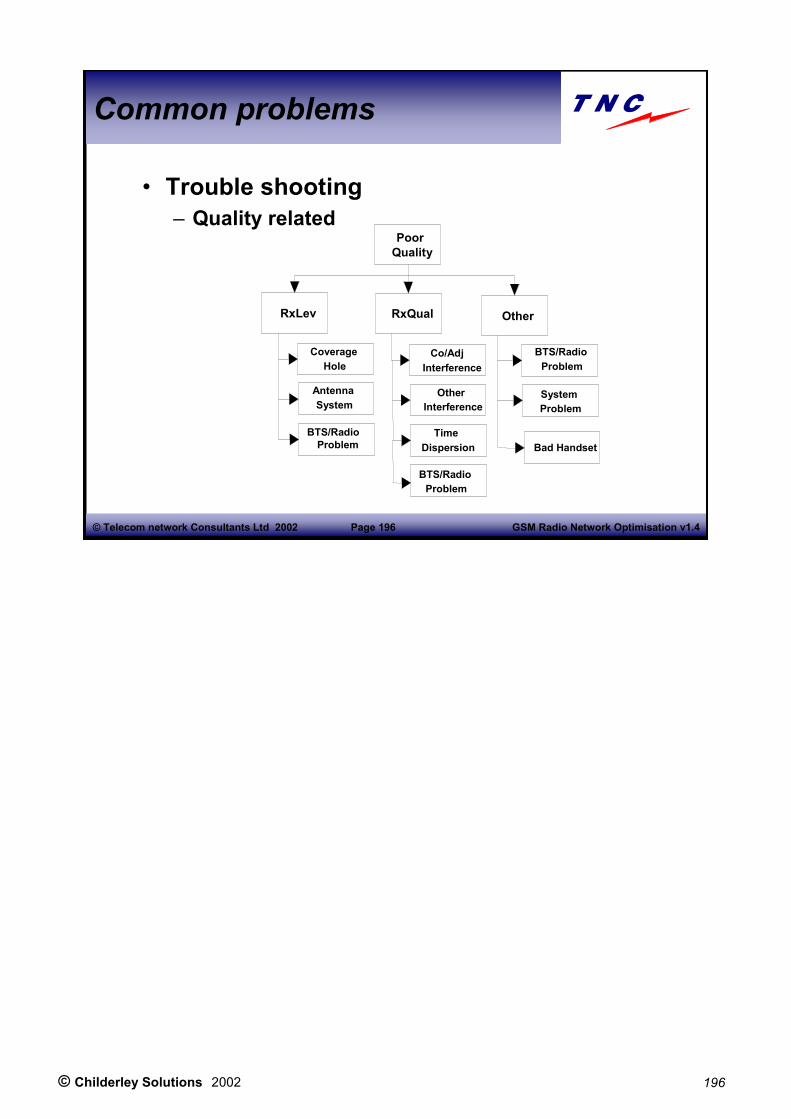
© Childerley Solutions 2002 196
GSM Radio Network Optimisation v1.4Page 196© Telecom network Consultants Ltd 2002
Common problems
• Trouble shooting – Quality related
Poor Quality
RxLev RxQual Other
Coverage Hole
Antenna System
BTS/RadioProblem
Co/AdjInterference
OtherInterference
Time Dispersion
BTS/Radio Problem
BTS/Radio Problem
System Problem
Bad Handset

© Childerley Solutions 2002 197
GSM Radio Network Optimisation v1.4Page 197© Telecom network Consultants Ltd 2002
Common problems
• Trouble shooting
– Handover problems
Handover Problem
Cell Dragging
Handover Failure
Ping-Pong Handovers
Neighbour List
Hysteresis
Interference
BTS/Radio Problem
Neighbour List
BTS/Radio Problem
System Problem
No Best Server
Neighbour Cell Data
Hysteresis
BTS/Radio Problem
Congestion
BadRxLev/RxQual

© Childerley Solutions 2002 198
GSM Radio Network Optimisation v1.4Page 198© Telecom network Consultants Ltd 2002
Common problems
• Trouble shooting– Call setup Dropped
Calls
RxLev RxQual Other
Coverage Hole
Handover Problem
Antenna System
BTS/Radio Problem
Co/AdjInterference
Other Interference
Time Dispersion
BTS/Radio Problem
BTS/Radio Problem
System Problem
BSS Parameters
Bad Handset

© Childerley Solutions 2002 199
GSM Radio Network Optimisation v1.4Page 199© Telecom network Consultants Ltd 2002
Common problems - review
• Interference• Missing neighbours• Multiple servers• Blocking• Failed handovers
© Childerley Solutions 2002 200
GSM Radio Network Optimisation v1.4Page 200© Telecom network Consultants Ltd 2002
Contents
• Optimisation Measures– Antenna Adjustments– Frequency & Interference Planning– Neighbour List Planning– Common Problems�Advanced Techniques

© Childerley Solutions 2002 201
GSM Radio Network Optimisation v1.4Page 201© Telecom network Consultants Ltd 2002
Advanced techniques
• Dynamic frequency planning• Smart antennas• Underlay/Overlay• Dual band networks• National roaming

© Childerley Solutions 2002 202
GSM Radio Network Optimisation v1.4Page 202© Telecom network Consultants Ltd 2002
Advanced techniques
• Dynamic frequency planning– Use OMC data to auto-optimise a frequency plan
– BCCH neighbour measurements– On hopping frequencies these neighbours are also interferers
– Don’t necessarily use 1/3 pattern with groups• Could have more of an ad-hoc plan
Some advanced frequency planning ideas with application particularly to hopping networks are in the “research” phases. Many different ideas are being put forward, as can be established by visiting the conferences.

© Childerley Solutions 2002 203
GSM Radio Network Optimisation v1.4Page 203© Telecom network Consultants Ltd 2002
Advanced techniques
• Smart antennas– Electrically steerable beam patterns– Steer a null towards an interferer– Antennas themselves expensive– Control a nightmare
• Each mobile link has a different interferer• With FH each TDMA frame is a different interferer• More potential for CDMA systems

© Childerley Solutions 2002 204
GSM Radio Network Optimisation v1.4Page 204© Telecom network Consultants Ltd 2002
Advanced techniques
• Underlay / overlay– Handover from inner to outer cells using special algorithm (interference triggered)
– Estimated 30% extra traffic• IF traffic density is highest close to the sites
D
R

© Childerley Solutions 2002 205
GSM Radio Network Optimisation v1.4Page 205© Telecom network Consultants Ltd 2002
Advanced techniques
• Dual band networks– 1800 MHz for capacity in cities– 900 MHz for coverage in rural areas– Coverage footprints different– Cell selection and handover should favour 1800MHz cells where possible
– Issue: one or two BCCHs per cell?

© Childerley Solutions 2002 206
GSM Radio Network Optimisation v1.4Page 206© Telecom network Consultants Ltd 2002
Advanced techniques
• National roaming– 1800MHz mobile selects 900MHz network when home network not available
• Exactly like international roaming• Need to reselect back to home network when possible
– Handover to 900MHz cell when 1800MHz handover not possible
• Only level triggered handover• Use priority handovers to favour 1800MHz cells

© Childerley Solutions 2002 207
GSM Radio Network Optimisation v1.4Page 207© Telecom network Consultants Ltd 2002
Advanced techniques - review
• Dynamic frequency planning• Smart antennas• Underlay/Overlay• Dual band networks• National roaming

© Childerley Solutions 2002 208
GSM Radio Network Optimisation v1.4Page 208© Telecom network Consultants Ltd 2002
Contents
• System Basics• BSS Parameters• Quality Assessment• Optimisation Measures�Organisation

© Childerley Solutions 2002 209
GSM Radio Network Optimisation v1.4Page 209© Telecom network Consultants Ltd 2002
Organisation
• Timetable• Teams• Preparation• Databases

© Childerley Solutions 2002 210
GSM Radio Network Optimisation v1.4Page 210© Telecom network Consultants Ltd 2002
Organisation
• Timetable– Coverage / capacity planning– Frequency planning– Neighbour planning– Parameter planning– “On-air”– Intensive optimisation– Ongoing optimisation
Networks undergoing regular expansion normally mature from the chaotic early days into a regular cycle of “long term planning” – “short term planning” – “optimisation”.
New sites are integrated into the network at regular, or at least pre-agreed intervals, followed by a short period of very intensive optimisation work to convert the planned network into one which meets the quality targets while carrying the planned amount of traffic.

© Childerley Solutions 2002 211
GSM Radio Network Optimisation v1.4Page 211© Telecom network Consultants Ltd 2002
Organisation
• Timetable
Turn-on-date
Frequencies and parameters
Drop-dead-date
Intensive optim
isation
3 month Traffic forecast
and TRX count
12 month Traffic forecast
and BS
count
New BS Planning
Ongoing optimisation
After a new turn on cycle a new frequency plan, neighbour plan and BSS parameter plan will be loaded into the network. To avoid negative impact on customers this is often done on a Friday night. Immediately following this is a period of intensive optimisation. Often it will involve working the whole weekend,, inn an attempt to ensure that on the Monday morning the initial call success rate target is met. (90% worst cell, 95% average)Ongoing optimisation will continue after this intensive optimisation period in order to raise the CSR to 95% in the worst cell and averaging better than 98%. However, the attention of the radio engineers will shift to longer and medium term expansion planning until the time comes to prepare for the next turn on cycle.The “drop dead date” is the final date at which sites must be listed for inclusion in the next ToC. After this the traffic and frequency planning activity will depend on having a stable network plan.

© Childerley Solutions 2002 212
GSM Radio Network Optimisation v1.4Page 212© Telecom network Consultants Ltd 2002
Organisation
• Teams– Quality
• Independent assessment of network quality• Drive tests• Network performance data
– Radio planning / Optimisation• Ideally within the same department• One person/small team responsible for an area of 50 to 100 sites
NB these functions are often organised differently within different operating companies (also at different times), but the basic functions remain.The quality department will monitor the network and report areas requiring attention to RF. Independent monitoring encourages RF to chase targets.Radio planning and optimisation ought to be within the same department, since all decisions in this area require trade-offs between quality (traditionally optimisation) and capacity (traditionally planning).

© Childerley Solutions 2002 213
GSM Radio Network Optimisation v1.4Page 213© Telecom network Consultants Ltd 2002
Organisation
• Teams– Drive testing
• Drivers and technicians/navigators• Resource available for Quality and Radio dept.
– Operations• Implementation of BSS parameters• Maintenance issues• Delivery of statistics
– Implementation• Build of new sites• Installation of TRX upgrades• Changes to antenna configurations
Drive test resource might be independent or in the quality department or in the RF department.
Operations, often have responsibility for the OMC. Their function is maintenance of the network, but this will often overlap with optimisation. The obvious area is where parameter changes are necessary.
Implementation will be making changes to antennas where necessary.

© Childerley Solutions 2002 214
GSM Radio Network Optimisation v1.4Page 214© Telecom network Consultants Ltd 2002
Organisation
• Preparation
– Cluster definition• Optimise manageable bits of the network• Edge of cluster should be an unchanged area
– BS testing• New sites should be tested for faults BEFORE optimisation
– Antennas connected correctly– Parameters set correctly – neighbours / BCCHs
An optimisation area, or cluster must be defined, so that a team can manage its work well. Ideally the network expansion and rollout will be organised so that the surrounding area will be not require optimising at the same time.
Many so called “optimisation problems” turn out to be hardware and software faults, incorrectly connected antennas or simple typos. Soon after the integration of new sites, they should be tested for functionality and correct configuration.

© Childerley Solutions 2002 215
GSM Radio Network Optimisation v1.4Page 215© Telecom network Consultants Ltd 2002
Organisation
• Preparation– Quality assessment
• Identify and locate problems
– Sources of data• Network performance statistics• Drive tests• Customer complaints
The first step in both the intensive optimisation stage and in the ongoing optimisation will be to identify the locations of network problems. Different methods of doing this each have their advantages and disadvantages. Network Performance Stats take time to collect and optimisation is usually scheduled for low traffic periodsDrive tests only measure downlink, unless linked to A-bis traces, which can be tedious.Customer complaints normally come after the end of the weekend, rather than early in the optimisation campaign, where it is desired to find all the problems.

© Childerley Solutions 2002 216
GSM Radio Network Optimisation v1.4Page 216© Telecom network Consultants Ltd 2002
Organisation
• Databases– Planning tool
• Current network situation• History• Plans
– Network• Live database of parameters• Antenna tilts and site locations
Database integrity is often difficult to maintain during an optimisation event. The problem is that settings and parameters are changing so quickly that it is sometimes difficult for the databases to keep up.
A direct link from planning tool to OMC can help. In the absence of this, and certainly for antenna changes, a disciplined change request procedure is required.

© Childerley Solutions 2002 217
GSM Radio Network Optimisation v1.4Page 217© Telecom network Consultants Ltd 2002
Organisation
• Databases– Measurements
• Large amounts of data• Catalogue to match with correct history database in planning tool
– Optimisation database• History of all optimisation problems and solutions• “Trouble ticket” system• Problems should be formally closed• Library of common problems for future help

© Childerley Solutions 2002 218
GSM Radio Network Optimisation v1.4Page 218© Telecom network Consultants Ltd 2002
Organisation
• Databases
– Optimisation database example
Problem Input- Operations- Qual. measurements- Custumer Complains- EmployeeProblemreports
DCS-Measurement
datas
-Logical Connection ofthe Measurement data tothe OptimisationProblem- Measurement data
DCS-Measurement
Request
- Optimisation Problem- Opt. Project Managment- Measurement Requests- Para.Change request forms- Optimisationproblem Solutions
Optimisation-database
Problemerfassung
ChangeRequestform
OptimisationReports
ToMeasurementteam
- To Fieldengineers- To OMC- To Radioplanning
Internal inOptimisation
Projekt Reports
Internal inOptimisation forProplemmanagement
DB Output
DB-Management
Map InfoGeographicalProblemdisplay
The optimisation database should be multi-user with a number of functions including:· Storage of information on problem originator· Prioritisation of problems· Logical connection of problems to Optimisation areas· Grouping of problems to a master/main problem· Storage of problem resolution measures· Printing of Change Requests and Measurement Requests· Historical record of Problems· Attachment of Win-files (pictures, documents) to a problem
The database could be configured as required, local to each region, which means that access will not be possible from another region or from a different location within the region. Each optimisation problem would still have a unique problem number, each new number being automatically assigned by the database. All measurement and change requests, optimisation and project reports will be generated in paper form. An administrator should be appointed to maintain the database, thereby ensuring the integrity over the lifetime of the network.

© Childerley Solutions 2002 219
GSM Radio Network Optimisation v1.4Page 219© Telecom network Consultants Ltd 2002
Organisation
• Implementation procedure– Identification of problems– Allocation of drive routes– Analysis of data– Solution of problems
• Check out side effects!!• Use planning tool• Liaise with other RF teams
– Implementation of solution– Verify solution

© Childerley Solutions 2002 220
GSM Radio Network Optimisation v1.4Page 220© Telecom network Consultants Ltd 2002
Organisation
Optimisation
Optimisation Guidelines Optimisation Database
Input Data collection:Metrica Statistics,Drive Test MeasurementsCustomer Complaints
Cluster Definition
Initial Site Validation
Data Analysis/Problem Identification
Solution Recommendationand Implementation
Validation of Solution
In a nutshell, the organisation that is established for optimisation is required to carry out these processes

© Childerley Solutions 2002 221
GSM Radio Network Optimisation v1.4Page 221© Telecom network Consultants Ltd 2002
Finally
• Take action ………
• Go optimise with confidence!

© Childerley Solutions 2002 222
GSM Radio Network Optimisation v1.4Page 222© Telecom network Consultants Ltd 2002
Contact details
Telecom Network ConsultantsHighfield House90 West DriveHighfields CaldecoteCambridge CB3 7NYTel: +44 1954 210841Fax: +44 1954 210840Email: [email protected]: www.tnc-ltd.com


![Untitled-2 []...˘ˇ ˆ ˙ ˇ ˙ ˝ ˛ ˚ˆ ˇ ˛ ˆ ˜ ˆ ˜ ˛ ˆˆ˙ !" # ˙ ˇ ˆ $ ˜ˆ ˆˆ $ ˛ ˙ ˛ ˛ ˆ ˆ ˜ ˆ ˆ $ ˝ ˛ ˚ˆ ˇ ˛ ˙ ˇ ˆ ˇˇ ˆˆ](https://img.pdfslide.us/doc/110x75/5e66db259e270c079278a430/untitled-2-oe-oe-.jpg)