A Comparison Study between Inferred State-Space and Neural Network Based System Identifications Using Adaptive Genetic Algorithm for Unmanned Helicopter Model

Proceedings of the 8th ICEENG Conference, 29-31 May, 2012 EE223 -

1

Military Technical College

Kobry El-Kobbah,

Cairo, Egypt

8th International Conference

on Electrical Engineering

ICEENG 2012

A Comparison Study between Inferred State-Space and Neural Network

Based System Identifications Using Adaptive Genetic Algorithm for

Unmanned Helicopter Model

By

Ahmed M. Hosny*

Abstract:

In this paper, system identifications of an unmanned aerial vehicle (UAV) based on

inferred state space and multiple neural networks were presented. In this work an

optimization approach was used to conclude an inferred state space and the multiple

neural networks system identifications based on the genetic algorithms separately. The

UAV is a multi-input multi-output (MIMO) nonlinear system. Models for such MIMO

system are expected to be adaptive to dynamic behavior and robust to environmental

variations. This task of accurate modeling has been achieved with multi-neural network

architecture in the most recent years. The presented work is focusing on an inferred state

space based system identification which is a new approach seldom used, but it is also

easier and more stable compared with the multi-network based system identification

during the modeling of dynamic behavior of nonlinear systems. In other words the

number of inputs used in the genetic algorithm to obtain an inferred state space is almost

one third of the number of inputs needed to develop the multi-layer recurrent neural

network architecture to simulate the required dynamic behavior of a real model. The

neural network models are based on the autoregressive technique with linear and

nonlinear networks. The simulation results presented in this paper show the superiority

of the inferred state space model compared with the autoregressive technique based

multi-neural network.

Keywords:

UAV Unmanned Aerial Vehicle, RC Remote Control, PI Performance Index, RNN

Recurrent Neural Network, GA Genetic Algorithm, ISS Inferred State Space.

ـــــــــــــــــــــــــــــــــــــــــــــــــــــــــــــــــــــــــــــــــــــــــــــــــــــــــــــــــــــــــــــــــــــــــــــــــــــــــــــــــــــــــــــــــ * Egyptian Armed Forces


2

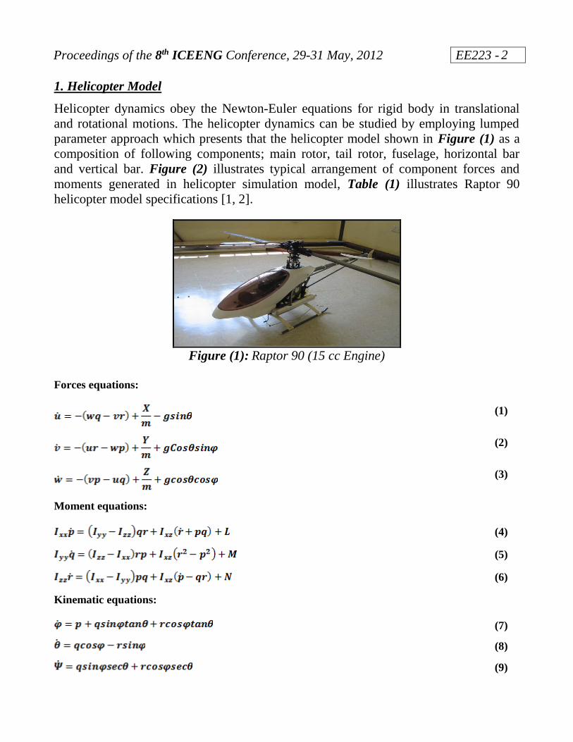
1. Helicopter Model

Helicopter dynamics obey the Newton-Euler equations for rigid body in translational

and rotational motions. The helicopter dynamics can be studied by employing lumped

parameter approach which presents that the helicopter model shown in Figure (1) as a

composition of following components; main rotor, tail rotor, fuselage, horizontal bar

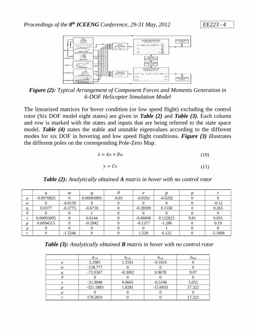
and vertical bar. Figure (2) illustrates typical arrangement of component forces and

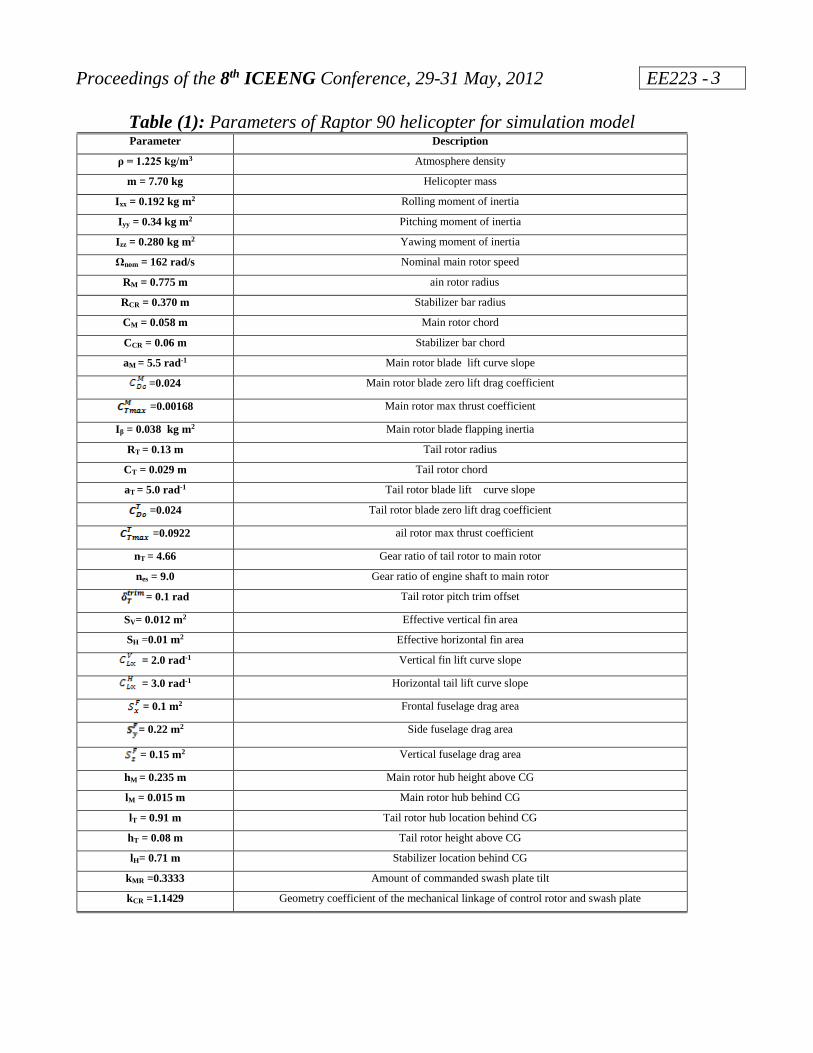
moments generated in helicopter simulation model, Table (1) illustrates Raptor 90

helicopter model specifications [1, 2].

Figure (1): Raptor 90 (15 cc Engine)

Forces equations:

(1)

(2)

(3)

Moment equations:

(4)

(5)

(6)

Kinematic equations:

(7)

(8)

(9)


3

Table (1): Parameters of Raptor 90 helicopter for simulation model Parameter Description

ρ = 1.225 kg/m3 Atmosphere density

m = 7.70 kg Helicopter mass

Ixx = 0.192 kg m2 Rolling moment of inertia

Iyy = 0.34 kg m2 Pitching moment of inertia

Izz = 0.280 kg m2 Yawing moment of inertia

Ωnom = 162 rad/s Nominal main rotor speed

RM = 0.775 m ain rotor radius

RCR = 0.370 m Stabilizer bar radius

CM = 0.058 m Main rotor chord

CCR = 0.06 m Stabilizer bar chord

aM = 5.5 rad-1 Main rotor blade lift curve slope

=0.024 Main rotor blade zero lift drag coefficient

=0.00168 Main rotor max thrust coefficient

Iβ = 0.038 kg m2 Main rotor blade flapping inertia

RT = 0.13 m Tail rotor radius

CT = 0.029 m Tail rotor chord

aT = 5.0 rad-1 Tail rotor blade lift curve slope

=0.024 Tail rotor blade zero lift drag coefficient

=0.0922 ail rotor max thrust coefficient

nT = 4.66 Gear ratio of tail rotor to main rotor

nes = 9.0 Gear ratio of engine shaft to main rotor

= 0.1 rad Tail rotor pitch trim offset

SV= 0.012 m2 Effective vertical fin area

SH =0.01 m2 Effective horizontal fin area

= 2.0 rad-1 Vertical fin lift curve slope

= 3.0 rad-1 Horizontal tail lift curve slope

= 0.1 m2 Frontal fuselage drag area

= 0.22 m2 Side fuselage drag area

= 0.15 m2 Vertical fuselage drag area

hM = 0.235 m Main rotor hub height above CG

lM = 0.015 m Main rotor hub behind CG

lT = 0.91 m Tail rotor hub location behind CG

hT = 0.08 m Tail rotor height above CG

lH= 0.71 m Stabilizer location behind CG

kMR =0.3333 Amount of commanded swash plate tilt

kCR =1.1429 Geometry coefficient of the mechanical linkage of control rotor and swash plate


4

Figure (2): Typical Arrangement of Component Forces and Moments Generation in

6-DOF Helicopter Simulation Model

The linearized matrices for hover condition (or low speed flight) excluding the control

rotor (Six DOF model eight states) are given in Table (2) and Table (3). Each column

and row is marked with the states and inputs that are being referred to the state space

model. Table (4) states the stable and unstable eigenvalues according to the different

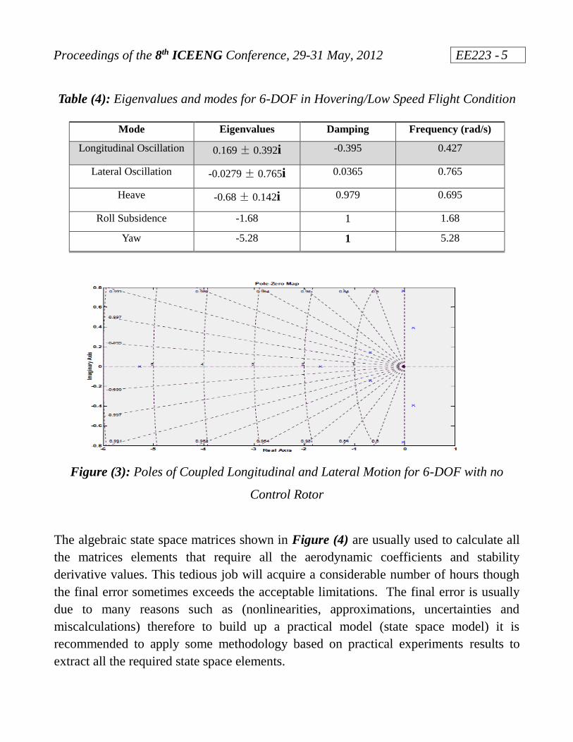
modes for six DOF in hovering and low speed flight conditions. Figure (3) illustrates

the different poles on the corresponding Pole-Zero Map.

(10)

(11)

Table (2): Analytically obtained A matrix in hover with no control rotor

u w q θ v p φ r

u -0.0070825 0 0.00093895 -9.81 -0.0292 -0.0292 0 0

w 0 -0.8159 0 0 0 0 0 -0.12

q 0.0377 -0.2775 -0.6718 0 -0.28599 0.1558 0 0.265

θ 0 0 1 0 0 0 0 0

v 0.00093895 0 0.0144 0 -0.06808 0.122823 9.81 0.055

p 0.0094513 0 -0.2942 0 -0.1377 -1.286 0 0.19

φ 0 0 0 0 0 1 0 0

r 0 -1.5246 0 0 1.528 0.122 0 -5.1868

Table (3): Analytically obtained B matrix in hover with no control rotor

δCol δLon δLat δPed

u 5.2981 1.5591 -0.1816 0

w -128.777 0 0 0

q -72.0367 -8.3082 0.9678 9.07

θ 0 0 0 0

v -31.9088 0.0605 -0.5196 5.055

p -321.1883 1.8281 -15.6933 17.322

φ 0 0 0 0

r 178.2831 0 0 17.322


5

Table (4): Eigenvalues and modes for 6-DOF in Hovering/Low Speed Flight Condition

Mode Eigenvalues Damping Frequency (rad/s)

Longitudinal Oscillation 0.169 ± 0.392i -0.395 0.427

Lateral Oscillation -0.0279 ± 0.765i 0.0365 0.765

Heave -0.68 ± 0.142i 0.979 0.695

Roll Subsidence -1.68 1 1.68

Yaw -5.28 1 5.28

Figure (3): Poles of Coupled Longitudinal and Lateral Motion for 6-DOF with no

Control Rotor

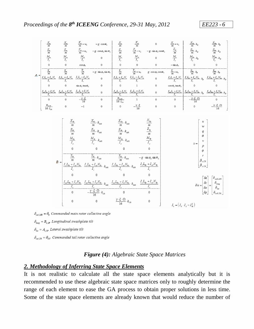
The algebraic state space matrices shown in Figure (4) are usually used to calculate all

the matrices elements that require all the aerodynamic coefficients and stability

derivative values. This tedious job will acquire a considerable number of hours though

the final error sometimes exceeds the acceptable limitations. The final error is usually

due to many reasons such as (nonlinearities, approximations, uncertainties and

miscalculations) therefore to build up a practical model (state space model) it is

recommended to apply some methodology based on practical experiments results to

extract all the required state space elements.


6

Figure (4): Algebraic State Space Matrices

2. Methodology of Inferring State Space Elements

It is not realistic to calculate all the state space elements analytically but it is

recommended to use these algebraic state space matrices only to roughly determine the

range of each element to ease the GA process to obtain proper solutions in less time.

Some of the state space elements are already known that would reduce the number of


7

the total elements. The unknown elements ranges only should be roughly determined in

order to decrease the number of iterations needed to obtain an acceptable solution that

represents the most global minimum of the performance index (the minimum error

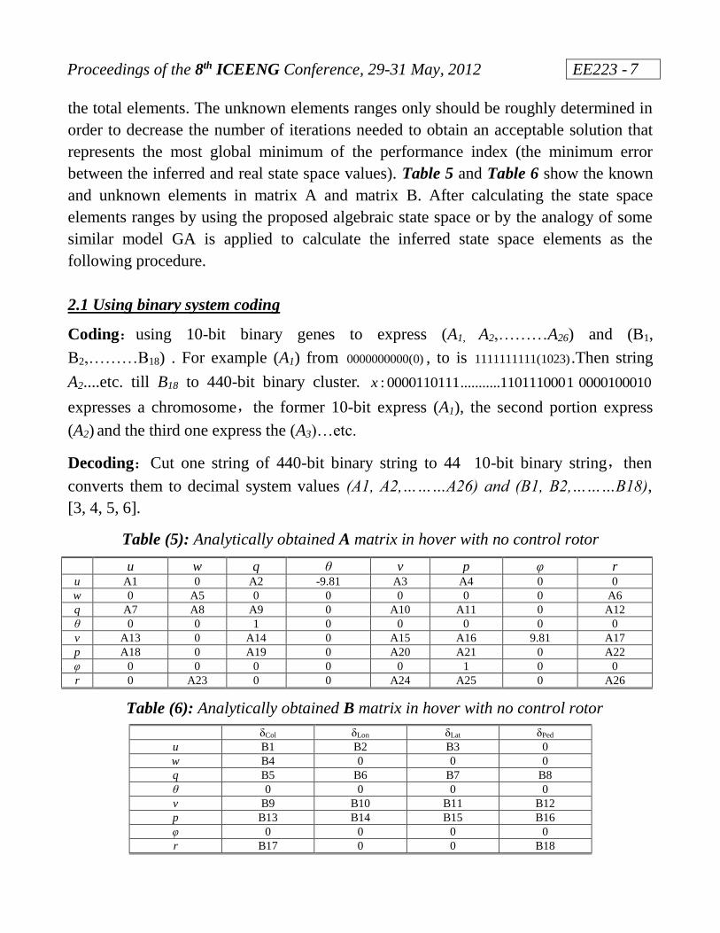
between the inferred and real state space values). Table 5 and Table 6 show the known

and unknown elements in matrix A and matrix B. After calculating the state space

elements ranges by using the proposed algebraic state space or by the analogy of some

similar model GA is applied to calculate the inferred state space elements as the

following procedure.

2.1 Using binary system coding

Coding：using 10-bit binary genes to express (A1, A2,………A26) and (B1,

B2,………B18) . For example (A1) from (0)0000000000 , to is (1023)1111111111 .Then string

A2....etc. till B18 to 440-bit binary cluster. 0000100010 1 110111000........... 0000110111:x

expresses a chromosome，the former 10-bit express (A1), the second portion express

(A2) and the third one express the (A3)…etc.

Decoding：Cut one string of 440-bit binary string to 44 10-bit binary string，then

converts them to decimal system values (A1, A2,………A26) and (B1, B2,………B18),

[3, 4, 5, 6].

Table (5): Analytically obtained A matrix in hover with no control rotor

u w q θ v p φ r u A1 0 A2 -9.81 A3 A4 0 0

w 0 A5 0 0 0 0 0 A6

q A7 A8 A9 0 A10 A11 0 A12

θ 0 0 1 0 0 0 0 0

v A13 0 A14 0 A15 A16 9.81 A17

p A18 0 A19 0 A20 A21 0 A22

φ 0 0 0 0 0 1 0 0

r 0 A23 0 0 A24 A25 0 A26

Table (6): Analytically obtained B matrix in hover with no control rotor

δCol δLon δLat δPed

u B1 B2 B3 0

w B4 0 0 0

q B5 B6 B7 B8

θ 0 0 0 0

v B9 B10 B11 B12

p B13 B14 B15 B16

φ 0 0 0 0

r B17 0 0 B18


8

2.2 Evaluation of fitness function

Fitness function is the main criterion of the GA algorithm, as it represents how much the

system is optimum and stable. The following equation describes the relation between

the fitness function and the performance index as shown in the following equation.

(11)

In the above equation is the actual system output while is the predicted output

(Inferred State Space), gk is the corresponding attitude weight that depends on the

priorities of this attitude. k is attitude notation corresponding to the states in the state

space matrix A. Therefore the fitness function could be written as the inverse of the

performance index of the inferred state space performance as shown in the following

equations. [9, 10, 11]

F(A1, A2,………A26, B1, B2,………B18 ) =(PI2)-1 (12)

2.3 Design operators

Proportion selection operator，single point crossover operator，basic bit mutation

operator.

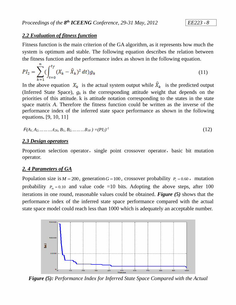
2. 4 Parameters of GA

Population size is 200M , generation 100G , crossover probability 0.60c P ，mutation

probability 0.10m P and value code =10 bits. Adopting the above steps, after 100

iterations in one round, reasonable values could be obtained. Figure (5) shows that the

performance index of the inferred state space performance compared with the actual

state space model could reach less than 1000 which is adequately an acceptable number.

Figure (5): Performance Index for Inferred State Space Compared with the Actual


9

3-Recurrent Neural Network Based System Identification

Different neural network structures and training methods were conducted for modeling

the nonlinear dynamics of the UAV. The ARX technique proved to be most suitable for

this purpose [7]. In the autoregressive neural network model the network retains

information about the previous outputs and inputs to predict the next output. This

provides equivalent retention capabilities of the dynamics of the UAV by the network.

The predicted output of a nonlinear model can be obtained as shown in the following

equation. [8]

(13)

Where θ is the coefficient matrix which gives the influence of past outputs (a.......ana)

and influence of past inputs (b1……b nb) on each of the subsequent outputs. The

nonlinear function is defined by g, the y and u terms correspond to past outputs and past

inputs respectively. The above equation can be simplified as

(14)

(15)

(16)

Here φ is the matrix of past inputs and outputs called the regressor and it is available

from memory. To obtain the coefficients θ, many assumptions and detailed knowledge

of the plant are necessary. Hence for a dynamic nonlinear system such as the UAV it

may not be feasible. This can be avoided by using black-box methods such as the neural

networks. The output of a two layered neural network is given as:

(17)


10

In the above equation F and G are the activation functions, l1 and l2 the number of

neurons in the two layers, b1j0 and b2j0 are the bias to the two layers and xk is the

network input. In most of the cases the nonlinearities are best represented by the

hyperbolic tangent function as the activation function G and a linear relation F. W1jk

and W2ij are the weights from the hidden layer and the output layer respectively. These

weights correspond to the θ matrix. Hence the problem of obtaining the best prediction

depends on the network structure adapted and the training method used. Iterative

training is performed to minimize an error function using the genetic algorithms. The

goal of the training is to obtain the most suitable values of weights for the closest

possible prediction output through repetitive iterations. The GA method works on the

principle of minimizing the mean squared error between the actual output of the system

and the predicted output of the network. The summation of the mean square error of

each subsequent attitude PI1 (performance index) should be minimized by applying GA.

3.1 Using binary system coding

Coding：using 20-bit binary genes to express (W1, W2,………W140) and (b1,

b2,………b13). For example (W1) from (0)00000000000000000000 , is

(1048575)11111111111111111111 .Then string W2....etc. till b13 to 3060-bit binary cluster.

0000100010 1 110111000........... 0000110111:x expresses a chromosome，the former 20-bit

express (W1), the second portion express (W2) and the third one express the (W3)…etc.

Decoding：Cut one string of 3060-bit binary string to 306 20-bit binary string，then

converts them to decimal system values (W1, W2,………W140) and (b1, b2,………b13) [3,

4].

3.2 Evaluation of fitness function

Fitness function is the main criterion of the GA algorithm, as it represents how much the

system is optimum and stable. The following equation describes the relation between

the fitness function and the performance index as shown in the following equation.

(18)

In the above equation is the actual system output while is the predicted output

(Recurrent Neural Network), gk is the corresponding attitude weight that depends on the


11

priorities of this attitude. k is the attitude notation in the state space matrix A. therefore

the fitness function could be written as the inverse of the performance index of the

recurrent neural network performance as shown in the following equation.

F(W1, W2,………W140, b1, b2,………b13) =(PI1)-1 (19)

3. 3 Design operators

Proportion selection operator，single point crossover operator，basic bit mutation

operator.

3. 4 Parameters of GA

Population size is 200M , generation 6000G at least, crossover probability

0.60c P ，mutation probability 0.10m P and cluster length =20 bits. Adopting the above

steps, consequently after 6000 steps iterations in five rounds a reasonable network

performance could be obtained compared with the actual system as shown in Table (7).

Table (7): Five Iterative Rounds for Weight Calculation

Round no. Adapted Weight Range ( multiplied by the best

weights from the previous process)

PI1

1 Predefined Weight Range 23000

2 The Best Weights in round (1) *0.3 19500





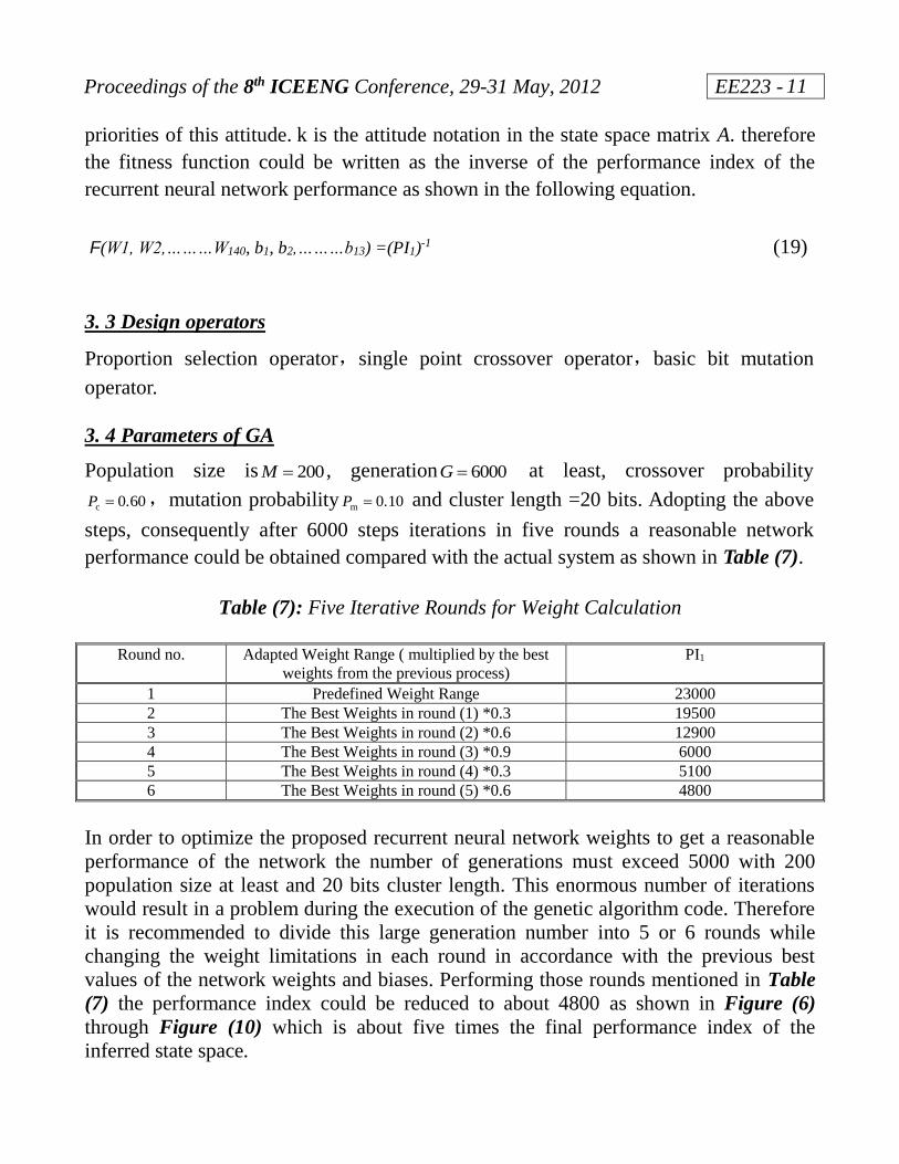
In order to optimize the proposed recurrent neural network weights to get a reasonable

performance of the network the number of generations must exceed 5000 with 200

population size at least and 20 bits cluster length. This enormous number of iterations

would result in a problem during the execution of the genetic algorithm code. Therefore

it is recommended to divide this large generation number into 5 or 6 rounds while

changing the weight limitations in each round in accordance with the previous best

values of the network weights and biases. Performing those rounds mentioned in Table

(7) the performance index could be reduced to about 4800 as shown in Figure (6)

through Figure (10) which is about five times the final performance index of the

inferred state space.


12

Figure (6): Performance Index in Round (1)





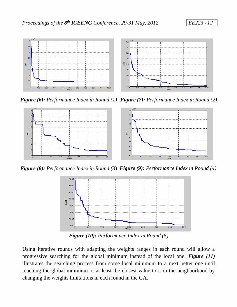
Using iterative rounds with adapting the weights ranges in each round will allow a

progressive searching for the global minimum instead of the local one. Figure (11)

illustrates the searching process from some local minimum to a next better one until

reaching the global minimum or at least the closest value to it in the neighborhood by

changing the weights limitations in each round in the GA.


13

Figure (11): Looking for the Global Minimum by Using Adaptive Genetic Algorithm

4. System Evaluation

4.1 Evaluation Criteria

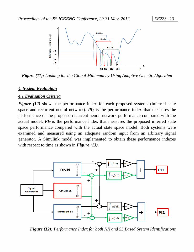
Figure (12) shows the performance index for each proposed systems (inferred state

space and recurrent neural network). PI1 is the performance index that measures the

performance of the proposed recurrent neural network performance compared with the

actual model. PI2 is the performance index that measures the proposed inferred state

space performance compared with the actual state space model. Both systems were

examined and measured using an adequate random input from an arbitrary signal

generator. A Simulink model was implemented to obtain these performance indexes

with respect to time as shown in Figure (13).

Figure (12): Performance Index for both NN and SS Based System Identifications


14

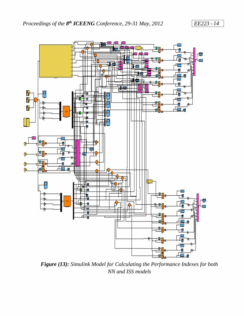
Figure (13): Simulink Model for Calculating the Performance Indexes for both

NN and ISS models


15

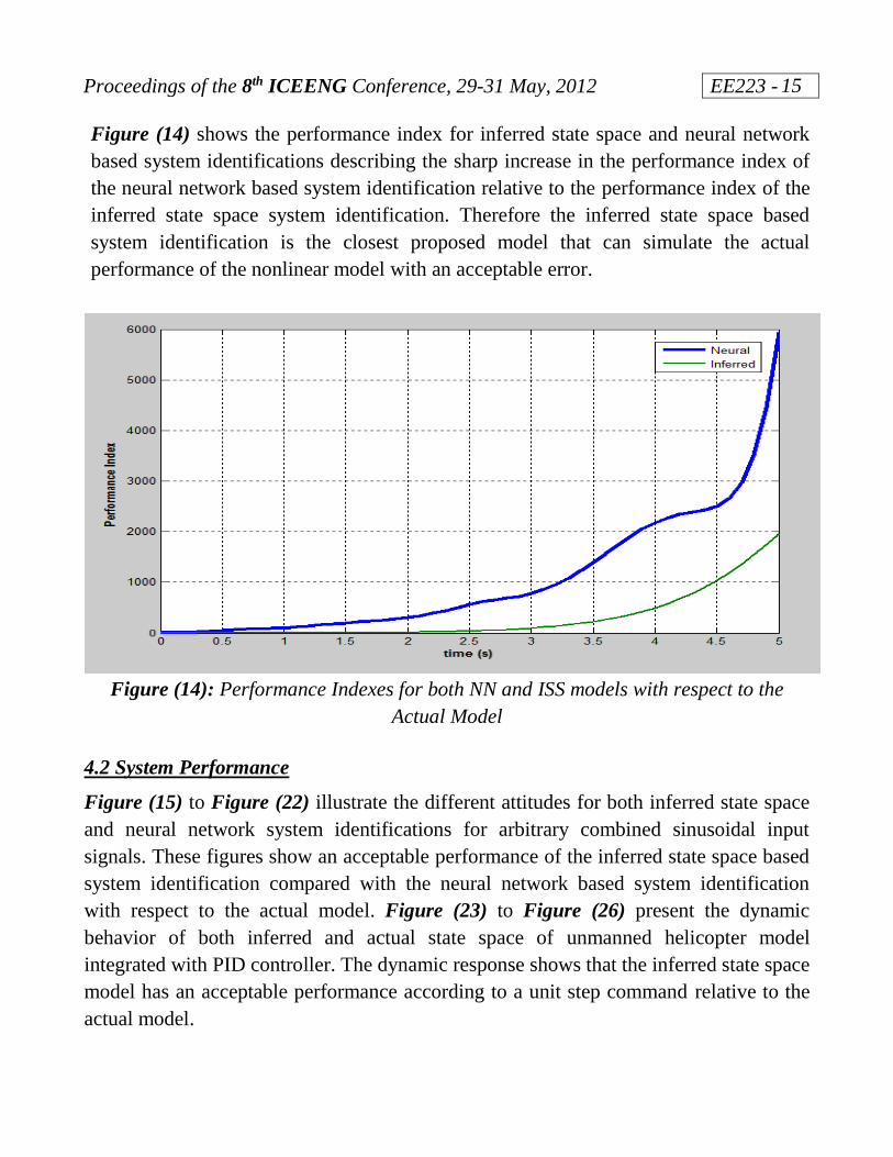
Figure (14) shows the performance index for inferred state space and neural network

based system identifications describing the sharp increase in the performance index of

the neural network based system identification relative to the performance index of the

inferred state space system identification. Therefore the inferred state space based

system identification is the closest proposed model that can simulate the actual

performance of the nonlinear model with an acceptable error.

Figure (14): Performance Indexes for both NN and ISS models with respect to the

Actual Model

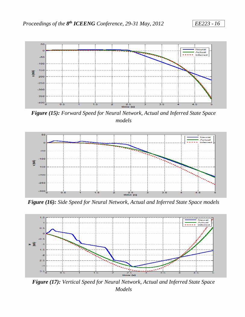
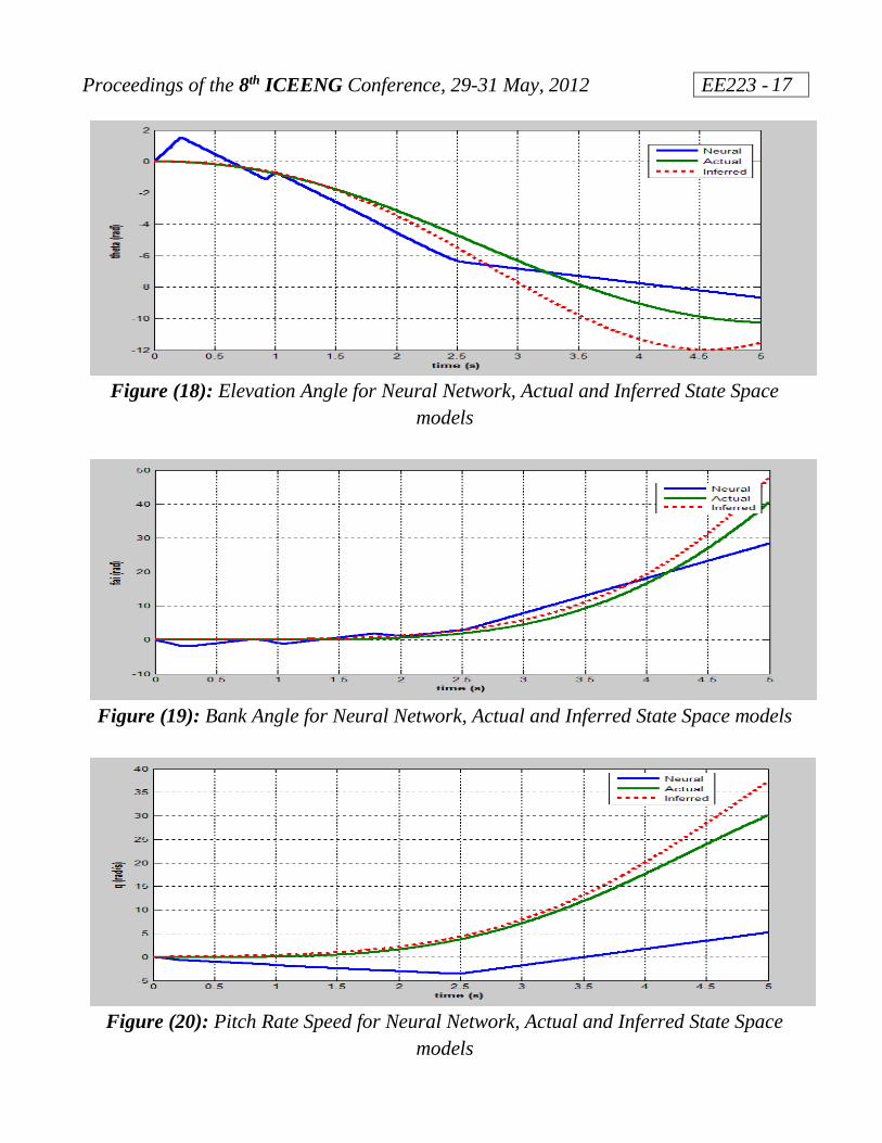
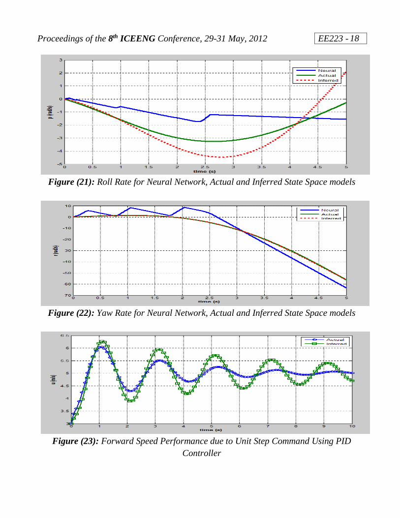
4.2 System Performance

Figure (15) to Figure (22) illustrate the different attitudes for both inferred state space

and neural network system identifications for arbitrary combined sinusoidal input

signals. These figures show an acceptable performance of the inferred state space based

system identification compared with the neural network based system identification

with respect to the actual model. Figure (23) to Figure (26) present the dynamic

behavior of both inferred and actual state space of unmanned helicopter model

integrated with PID controller. The dynamic response shows that the inferred state space

model has an acceptable performance according to a unit step command relative to the

actual model.


16

Figure (15): Forward Speed for Neural Network, Actual and Inferred State Space

models

Figure (16): Side Speed for Neural Network, Actual and Inferred State Space models

Figure (17): Vertical Speed for Neural Network, Actual and Inferred State Space

Models


17

Figure (18): Elevation Angle for Neural Network, Actual and Inferred State Space

models

Figure (19): Bank Angle for Neural Network, Actual and Inferred State Space models

Figure (20): Pitch Rate Speed for Neural Network, Actual and Inferred State Space

models


18

Figure (21): Roll Rate for Neural Network, Actual and Inferred State Space models

Figure (22): Yaw Rate for Neural Network, Actual and Inferred State Space models

Figure (23): Forward Speed Performance due to Unit Step Command Using PID

Controller


19

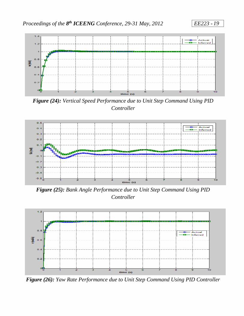
Figure (24): Vertical Speed Performance due to Unit Step Command Using PID

Controller

Figure (25): Bank Angle Performance due to Unit Step Command Using PID

Controller

Figure (26): Yaw Rate Performance due to Unit Step Command Using PID Controller


20

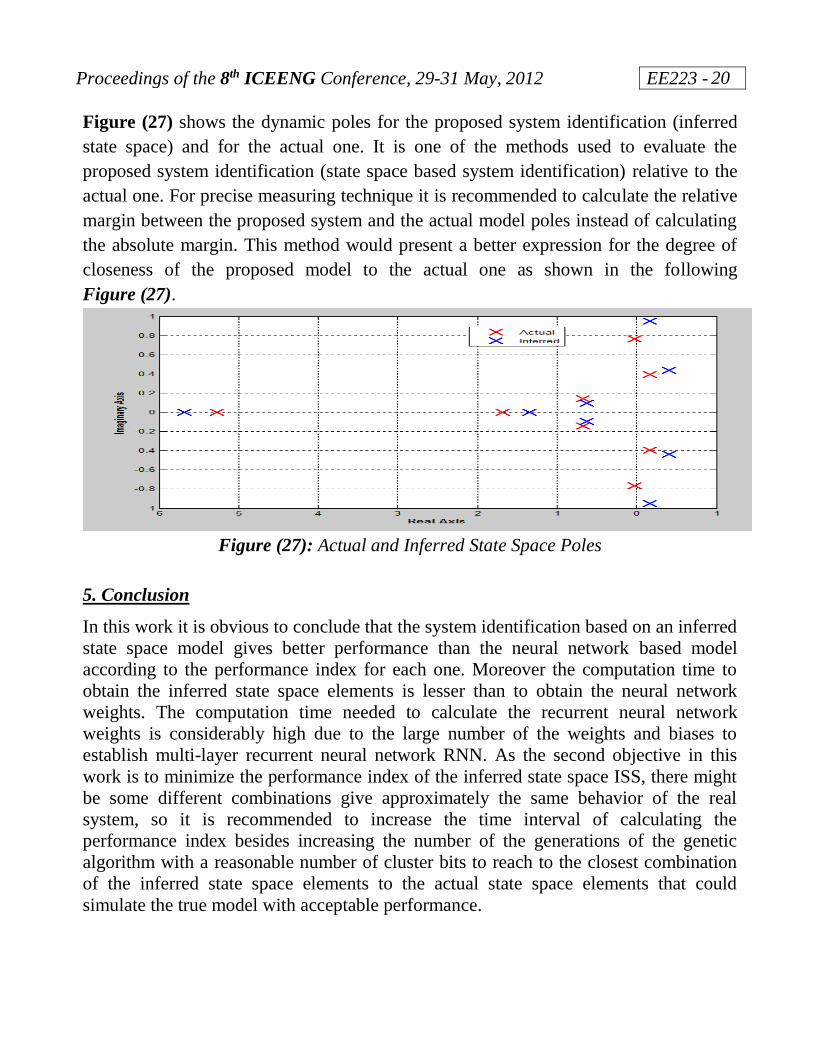
Figure (27) shows the dynamic poles for the proposed system identification (inferred

state space) and for the actual one. It is one of the methods used to evaluate the

proposed system identification (state space based system identification) relative to the

actual one. For precise measuring technique it is recommended to calculate the relative

margin between the proposed system and the actual model poles instead of calculating

the absolute margin. This method would present a better expression for the degree of

closeness of the proposed model to the actual one as shown in the following

Figure (27).

Figure (27): Actual and Inferred State Space Poles

5. Conclusion

In this work it is obvious to conclude that the system identification based on an inferred

state space model gives better performance than the neural network based model

according to the performance index for each one. Moreover the computation time to

obtain the inferred state space elements is lesser than to obtain the neural network

weights. The computation time needed to calculate the recurrent neural network

weights is considerably high due to the large number of the weights and biases to

establish multi-layer recurrent neural network RNN. As the second objective in this

work is to minimize the performance index of the inferred state space ISS, there might

be some different combinations give approximately the same behavior of the real

system, so it is recommended to increase the time interval of calculating the

performance index besides increasing the number of the generations of the genetic

algorithm with a reasonable number of cluster bits to reach to the closest combination

of the inferred state space elements to the actual state space elements that could

simulate the true model with acceptable performance.


21

6. References

[1] Shamsudin S. S., “The Development of Autopilot System for an Unmanned Aerial

Vehicle (UAV) Helicopter Model”, "University of Technology, M.Sc." August,

2007, pp. 1-147.

[2] Hosny A. M., Chao H., “ Development of Fuzzy Logic LQR Control Integration

for Aerial Refueling Autopilot”, " Proceedings of the 12th International Conference

on Aerospace Sciences and Aviation Technology, ASAT-12," May 29-31, 2007.

[3] Hosny A. M., Chao H., “Fuzzy Logic Controller Tuning Via Adaptive Genetic

Algorithm Applied to Aircraft Longitudinal Motion”, " Proceedings of the 12th

International Conference on Aerospace Sciences and Aviation Technology, ASAT-

12," May 29-31, 2007.

[4] Goldberg, D., Genetic Algorithms in Search, Optimization & Machine Learning,1st.

ed., Vol. 1, Addison Wesley Longman, 1989.

[5] Flying Qualities of Aeronautical Design Standard for military helicopter (ADS-

33C) (US Army Aviation Systems Command, 1989).

[6] Hosny A. M., Hosny M. M. and Ez El-Deen H., “Development of a Customized

Autopilot for Unmanned Helicopter Model Using Genetic Algorithm via the

Application of Different Guidance Strategies” International Conference on

Aerospace Sciences and Aviation Technology, ASAT-14," May 24-26, 2011.

[7] Lennart Ljung, “System Identification - Theory for the User”, Prentice Hall, 2nd

edition, 1999, Prentice Hall, 2nd edition, 1999.

[8] Vishwas Puttige and Sreenatha Anavatti. “Real-time Neural Network Based Online

Identification Technique for a UAV Platform”, In International Conference on

Computational Intelligence for Modeling Control Application, page 92,

Washington, DC, USA, 2006, IEEE Computer Society.