Embed Size (px)
Citation preview
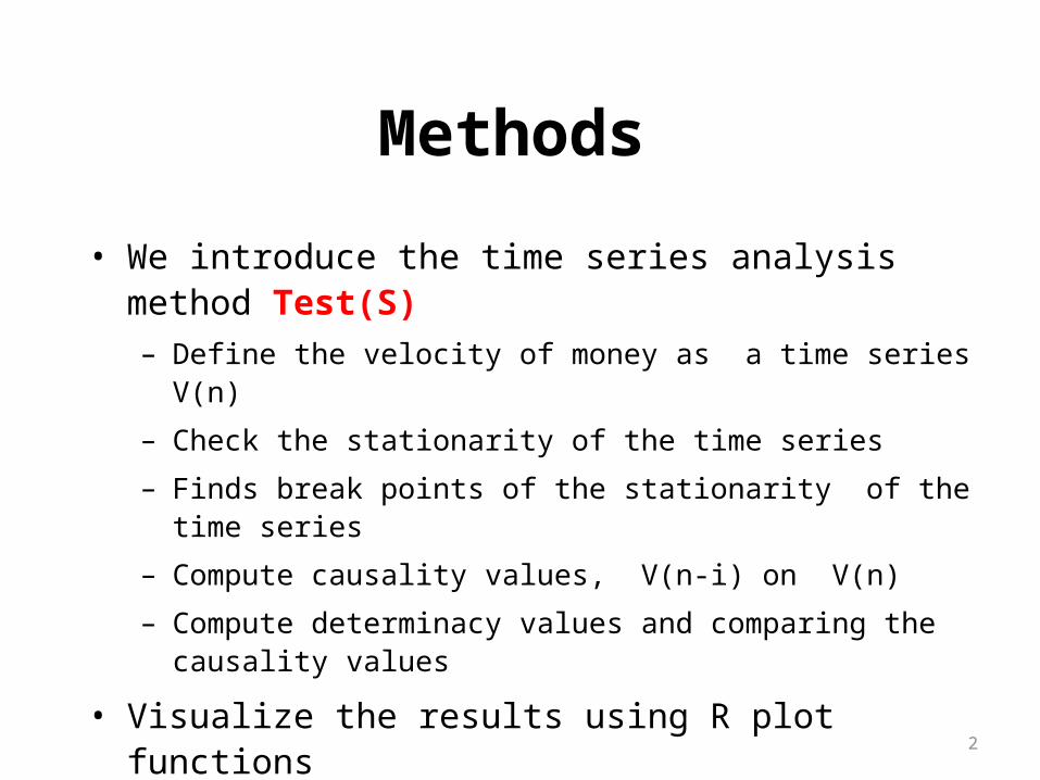
Methods
• We introduce the time series analysis method Test(S) – Define the velocity of money as a time series V(n)
– Check the stationarity of the time series
– Finds break points of the stationarity of the time series
– Compute causality values, V(n-i) on V(n)
– Compute determinacy values and comparing the causality values
• Visualize the results using R plot functions *This presentation is based on the paper [1.]
2
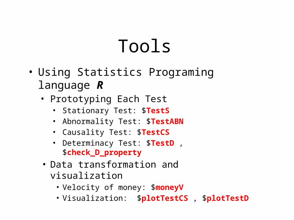
Tools• Using Statistics Programing language R
• Prototyping Each Test• Stationary Test: $TestS • Abnormality Test: $TestABN• Causality Test: $TestCS• Determinacy Test: $TestD , $check_D_property
• Data transformation and visualization• Velocity of money: $moneyV• Visualization: $plotTestCS , $plotTestD

History of Prototyping• These tests are developed as Basic Programs
• Prof Nakano[1], 1990 ~
• Converted to Java Programs• Saito , 2010 ~
• Developing R scripts ( using Rjava )
– Saito , 2012~
4

Introduction to the research
• In preparation
5
Outline
1. Money Velocity(1)2. Non linear transformation3. Stationary Test : $Test(S)4. Abnormality Test : $Test(ABN) 5. Money Velocity(2)6. Causality Test : $Test(CS)7. Determinacy Test: $test(D)
6
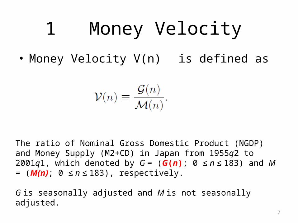
1 Money Velocity • Money Velocity V(n) is defined as
7
The ratio of Nominal Gross Domestic Product (NGDP) and Money Supply (M2+CD) in Japan from 1955q2 to 2001q1, which denoted by G = (G(n); 0 ≤ n ≤ 183) and M = (M(n); 0 ≤ n ≤ 183), respectively.
G is seasonally adjusted and M is not seasonally adjusted.
1 Money Velocity : Data Entry
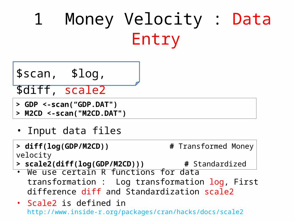
• Input data files
$scan, $log, $diff, scale2
> GDP <-scan(“GDP.DAT")> M2CD <-scan("M2CD.DAT")
• We use certain R functions for data transformation : Log transformation log, First difference diff and Standardization scale2
• Scale2 is defined in http://www.inside-r.org/packages/cran/hacks/docs/scale2
> diff(log(GDP/M2CD)) # Transformed Money velocity> scale2(diff(log(GDP/M2CD))) # Standardized
1 Money Velocity : Visualization
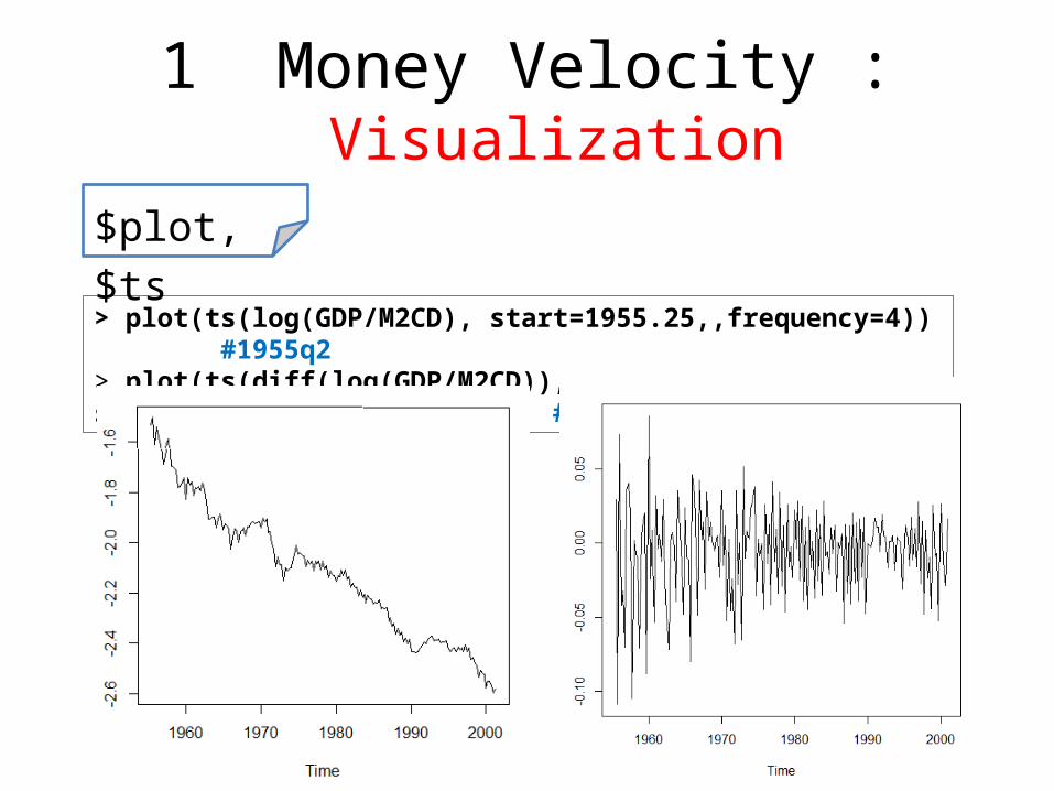
> plot(ts(log(GDP/M2CD), start=1955.25,,frequency=4)) #1955q2> plot(ts(diff(log(GDP/M2CD)), start=1955.5,,frequency=4)) #1955q3 (diff)
$plot, $ts
2 Non linear transformation
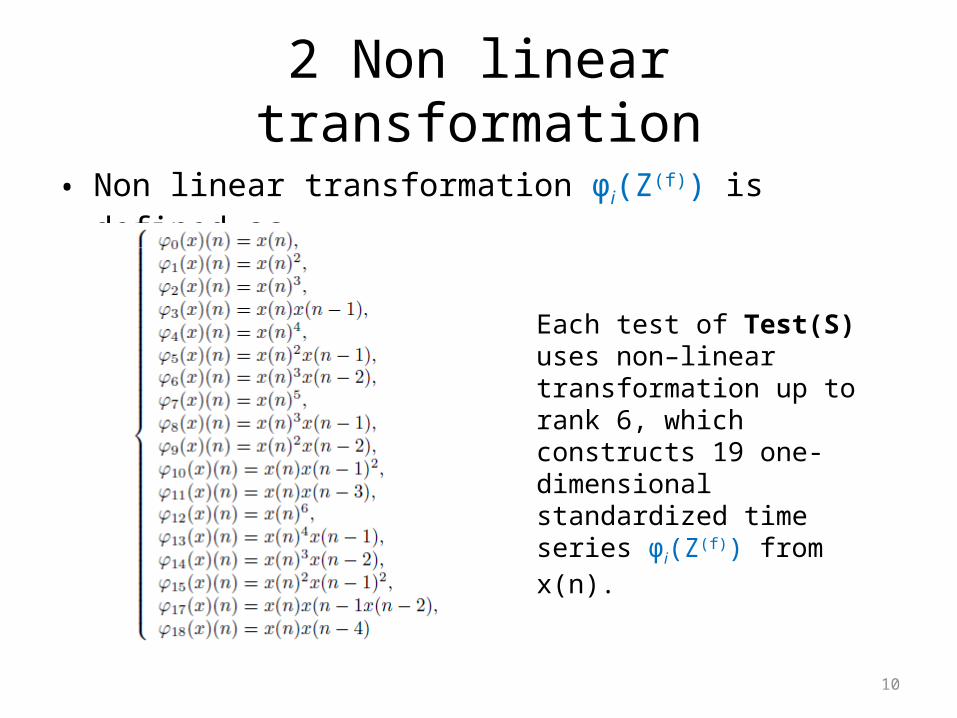
• Non linear transformation φi(Z(f)) is defined as
10
Each test of Test(S) uses non–linear transformation up to rank 6, which constructs 19 one-dimensional standardized time series φi(Z(f)) from x(n).
3 Stationary Test : Test(S)
• Test(S) tests the target time series X(n) is stationary or not– Test(S) is applied to a subsequence TERM of X(n)
– The length of TERM is set to 99: -> Economical Data
– Test(S) is passed if the result satisfies conditions describing later
• Test(S) is repeatedly applied by 19 times with respect to each φi(Z(f)) transformed from X(n)
– Each time series in φi(Z(f)) is tested and put a result respectively
• For examples “φ0(x), φ3(x), φ11(x), φ17(x) are passed by test(S) ”
11
4 Abnormality Test : Test(ABN)
• Test(ABN) Test the “degree of breaks in a time series”
• Repeats Test(S) about subsequence term , of which length is denoted as cutlength and set to 98.
• Test(ABN) returns a sequence of the Test(S) results– Detect the points N -> 0 (N: natural number)
12
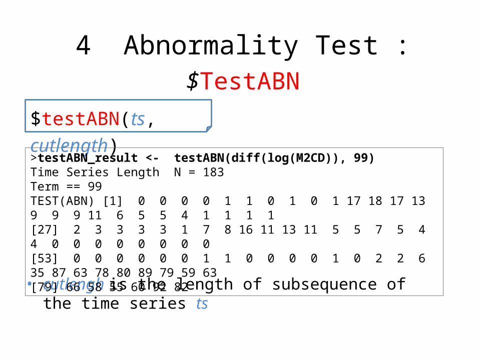
4 Abnormality Test : $TestABN
• cutlengh is the length of subsequence of the time series ts
$testABN(ts, cutlength)
>testABN_result <- testABN(diff(log(M2CD)), 99) Time Series Length N = 183Term == 99TEST(ABN) [1] 0 0 0 0 1 1 0 1 0 1 17 18 17 13 9 9 9 11 6 5 5 4 1 1 1 1[27] 2 3 3 3 3 1 7 8 16 11 13 11 5 5 7 5 4 4 0 0 0 0 0 0 0 0[53] 0 0 0 0 0 0 1 1 0 0 0 0 1 0 2 2 6 35 87 63 78 80 89 79 59 63[79] 66 58 55 60 92 82
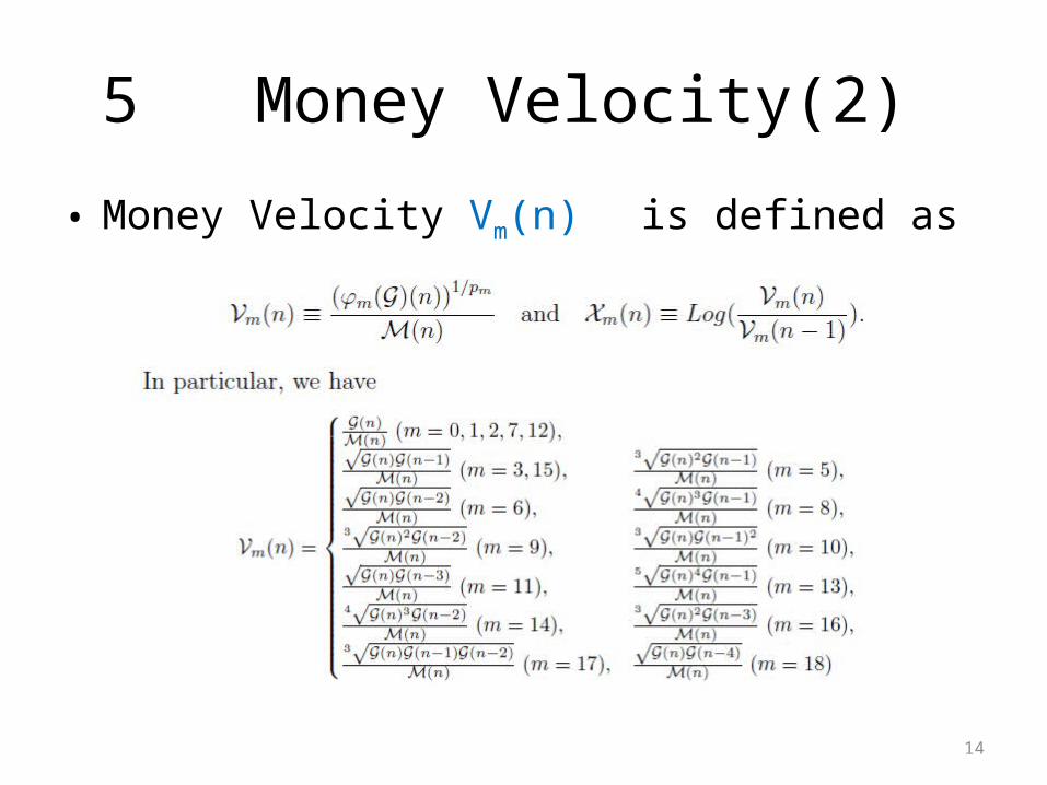
5 Money Velocity(2)
• Money Velocity Vm(n) is defined as
14
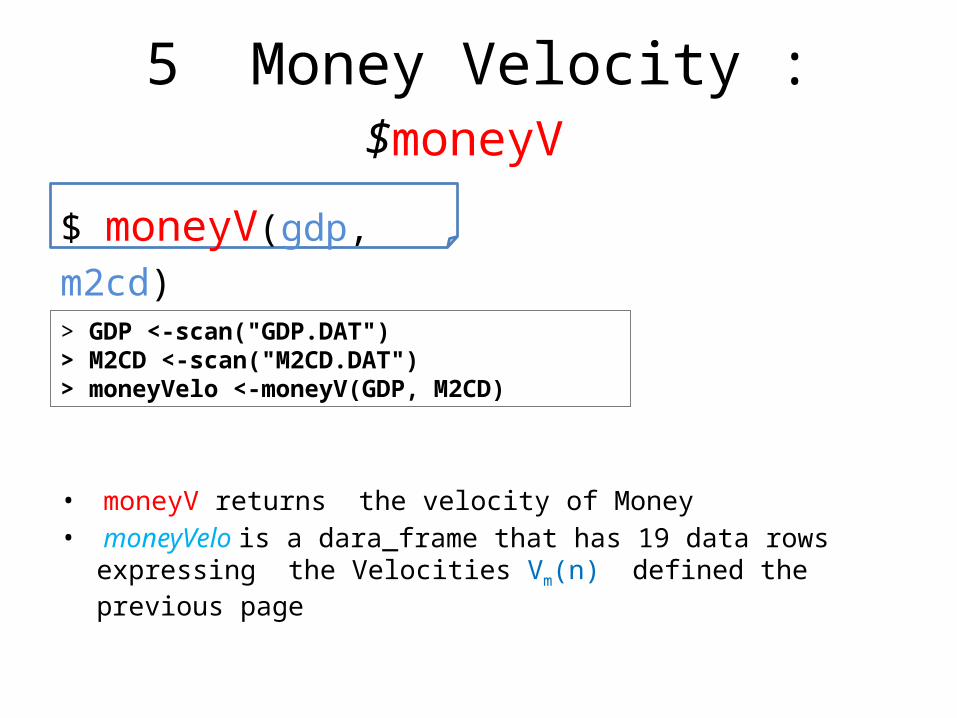
5 Money Velocity : $moneyV
• moneyV returns the velocity of Money• moneyVelo is a dara_frame that has 19 data rows expressing the
Velocities Vm(n) defined the previous page
$ moneyV(gdp, m2cd)
> GDP <-scan("GDP.DAT")> M2CD <-scan("M2CD.DAT")> moneyVelo <-moneyV(GDP, M2CD)
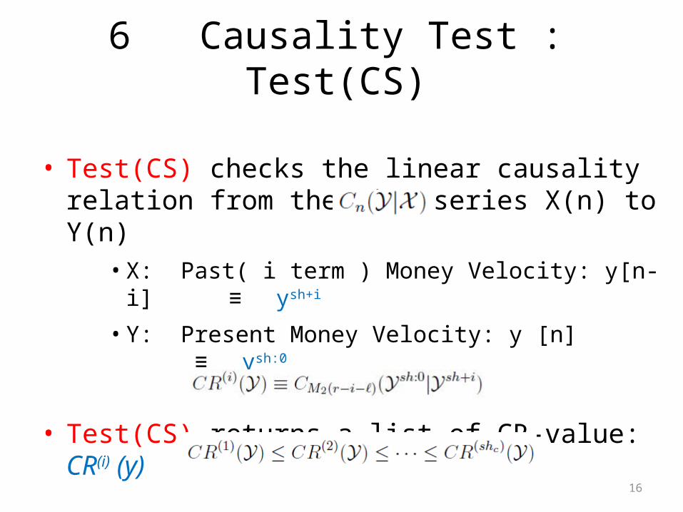
6 Causality Test : Test(CS)
• Test(CS) checks the linear causality relation from the time series X(n) to Y(n)
• X: Past( i term ) Money Velocity: y[n-i] ≡ ysh+i
• Y: Present Money Velocity: y [n] ≡ ysh:0
• Test(CS) returns a list of CR-value: CR(i) (y)
– The values are ordered as
16
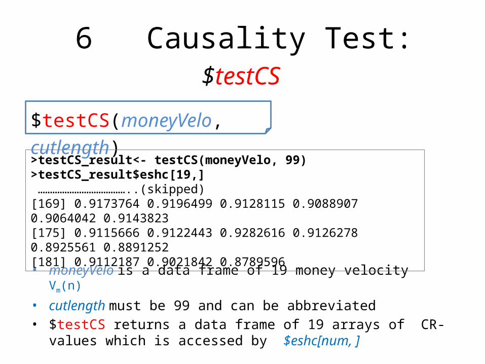
6 Causality Test: $testCS
• moneyVelo is a data frame of 19 money velocity Vm(n)
• cutlength must be 99 and can be abbreviated• $testCS returns a data frame of 19 arrays of CR-values which is accessed
by $eshc[num, ]
$testCS(moneyVelo, cutlength)
>testCS_result<- testCS(moneyVelo, 99)>testCS_result$eshc[19,] ………………………………..(skipped)[169] 0.9173764 0.9196499 0.9128115 0.9088907 0.9064042 0.9143823[175] 0.9115666 0.9122443 0.9282616 0.9126278 0.8925561 0.8891252[181] 0.9112187 0.9021842 0.8789596
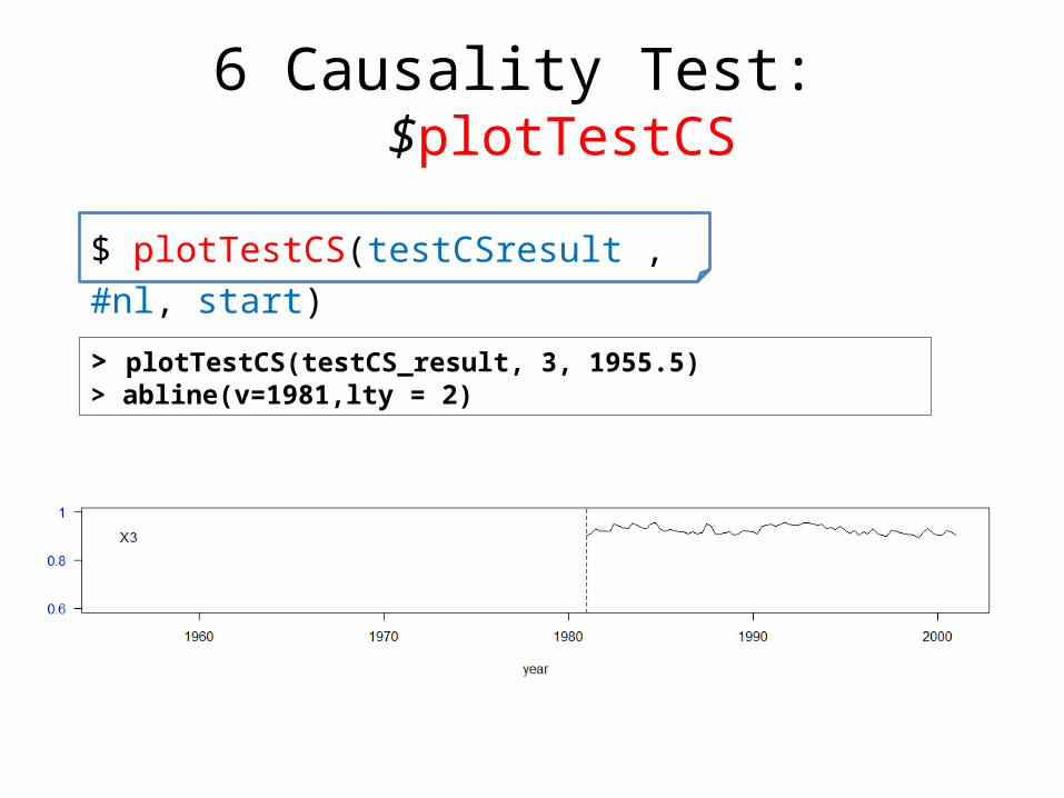
6 Causality Test: $plotTestCS
> plotTestCS(testCS_result, 3, 1955.5)> abline(v=1981,lty = 2)
$ plotTestCS(testCSresult , #nl, start)
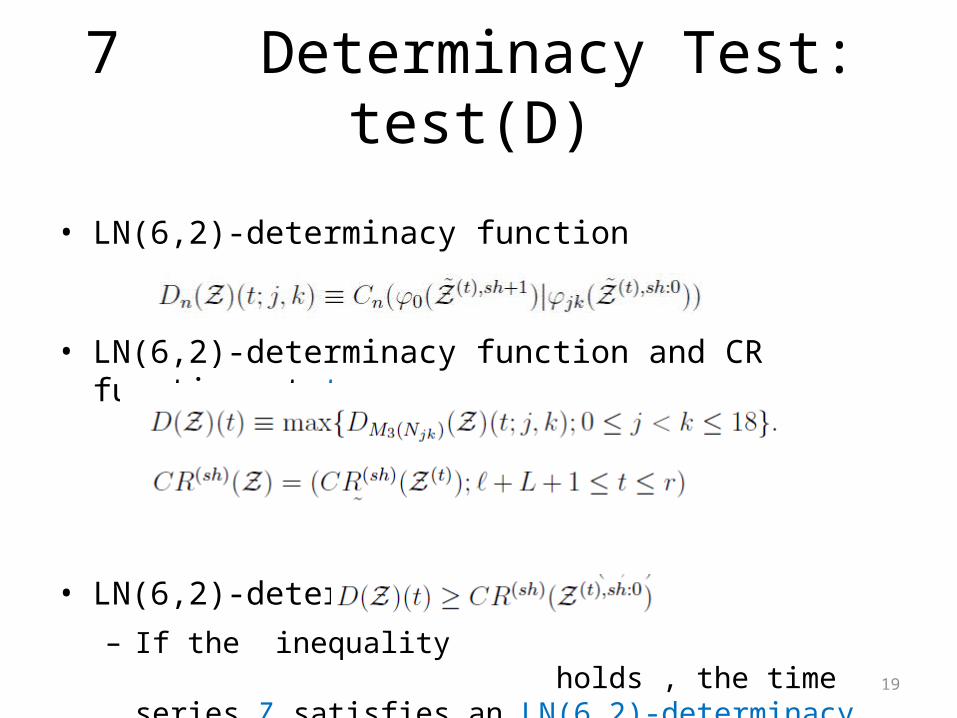
7 Determinacy Test: test(D)
• LN(6,2)-determinacy function
• LN(6,2)-determinacy function and CR function at t
• LN(6,2)-determinacy property– If the inequality holds , the time
series Z satisfies an LN(6,2)-determinacy property at the time t.
19
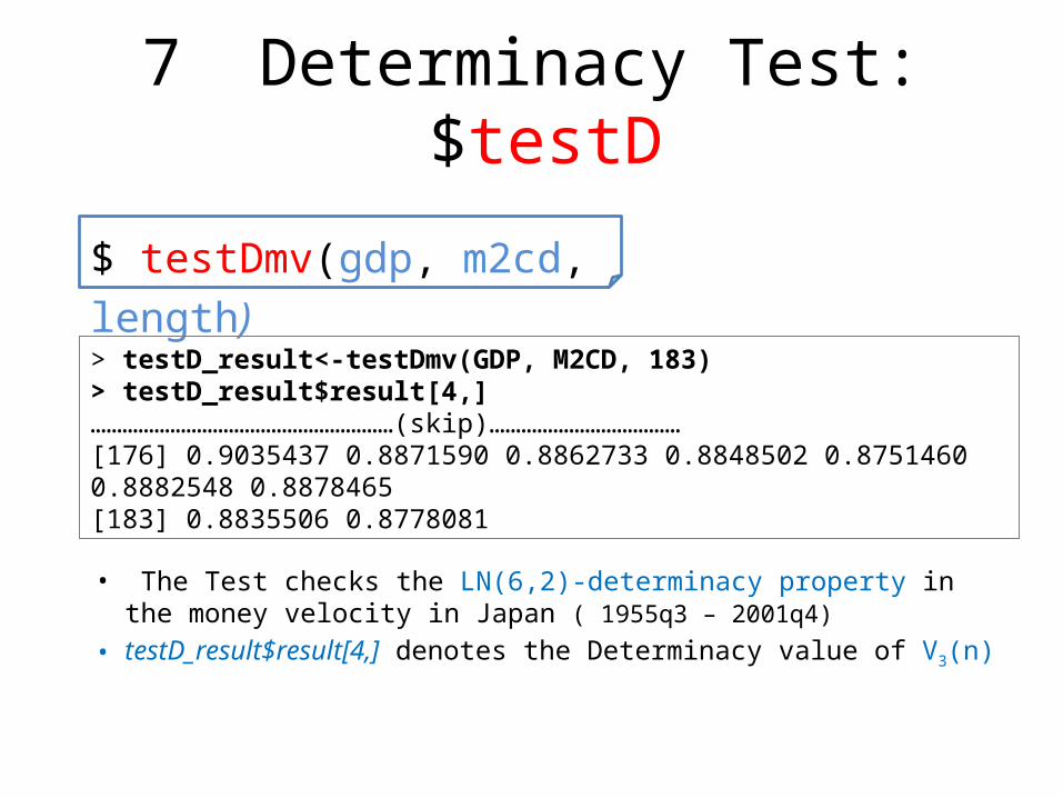
7 Determinacy Test: $testD
• The Test checks the LN(6,2)-determinacy property in the money velocity in Japan ( 1955q3 – 2001q4)
• testD_result$result[4,] denotes the Determinacy value of V3(n)
$ testDmv(gdp, m2cd, length)
> testD_result<-testDmv(GDP, M2CD, 183)> testD_result$result[4,]…………………………………………………(skip)………………………………[176] 0.9035437 0.8871590 0.8862733 0.8848502 0.8751460 0.8882548 0.8878465[183] 0.8835506 0.8778081
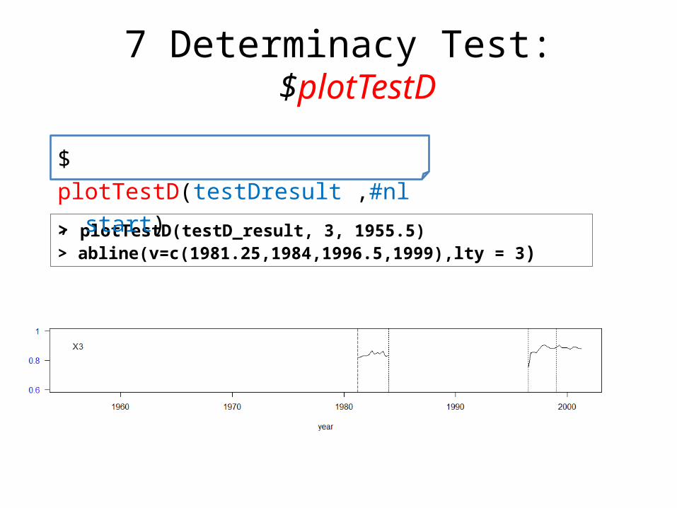
7 Determinacy Test: $plotTestD
> plotTestD(testD_result, 3, 1955.5)> abline(v=c(1981.25,1984,1996.5,1999),lty = 3)
$ plotTestD(testDresult ,#nl, start)
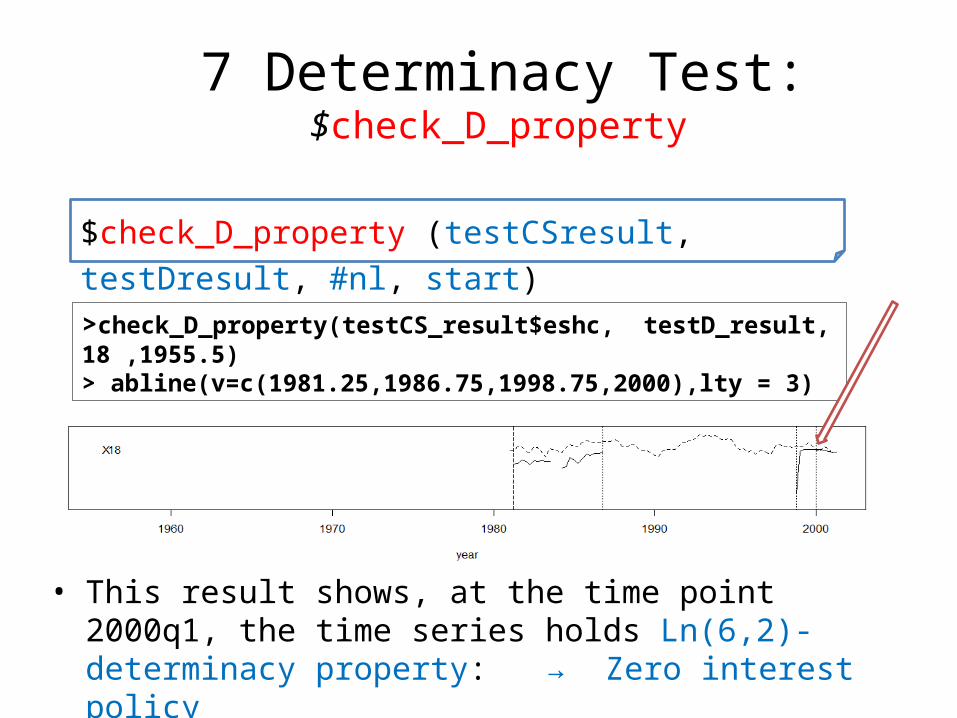
7 Determinacy Test: $check_D_property
>check_D_property(testCS_result$eshc, testD_result, 18 ,1955.5)> abline(v=c(1981.25,1986.75,1998.75,2000),lty = 3)
$check_D_property (testCSresult, testDresult, #nl, start)
• This result shows, at the time point 2000q1, the time series holds Ln(6,2)-determinacy property: → Zero interest policy – X18: 179(2000q1) testD_value=0.8975 > testCS_value=0.8923
Conclusion
• This is a provisional version
• We hope these Tests will be prevailed
23
References1. Yuji Nakano, Yasunori Okabe : A Time Series Analysis of Economical
Phenomena in Japan’s Lost Decade (1): Determinacy Property of the Velocity of Money and Equilibrium Solution ,Asia-Pacific Financial Markets November 2012, Volume 19, Issue 4, pp 371-389
24

Appendix
25
Conditions of Test(S)• Test the target time series X(n) is stationary or not
– Test(S) is applied to a subsequence TERM of X(n)
– The length of TERM is set to 99: Economical Data
– Test(S) is passed if the result satisfies conditions describing later
• Test(S) is repeatedly applied by 19 times with respect to ψi(Z(f)) transformed from X(n).
– Each time series in ψi(Z(f)) is tested respectively
• For examples “φ0(x), φ3(x), φ11(x), φ17(x) are passed by test(S) ”
26
Appendix (A)
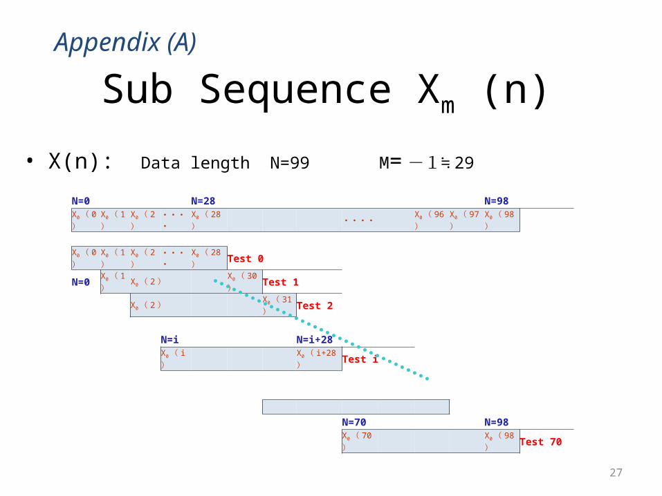
Sub Sequence Xm (n)
N=0 N=28 N=98 Χ0( 0
)Χ0( 1
)Χ0( 2
)・・・・
Χ0( 28
) ・・・・
Χ0( 96
)Χ0( 97
)Χ0( 98
)
Χ0( 0
)Χ0( 1
)Χ0( 2
)・・・・
Χ0( 28
)Test 0
N=0 Χ0( 1
)Χ0( 2) Χ0( 30
)Test 1
Χ0( 2)
Χ0( 31
)Test 2
N=i N=i+28Χ0( i
)
Χ0( i+28
)Test i
N=70 N=98 Χ0( 70
)
Χ0( 98
)Test 70
27
• X(n): Data length N=99 M= -1≒ 29
Appendix (A)
28
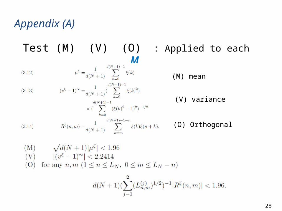
• Test (M) (V) (O) : Applied to each M
•
(M) mean
(V) variance
(O) Orthogonal
Appendix (A)
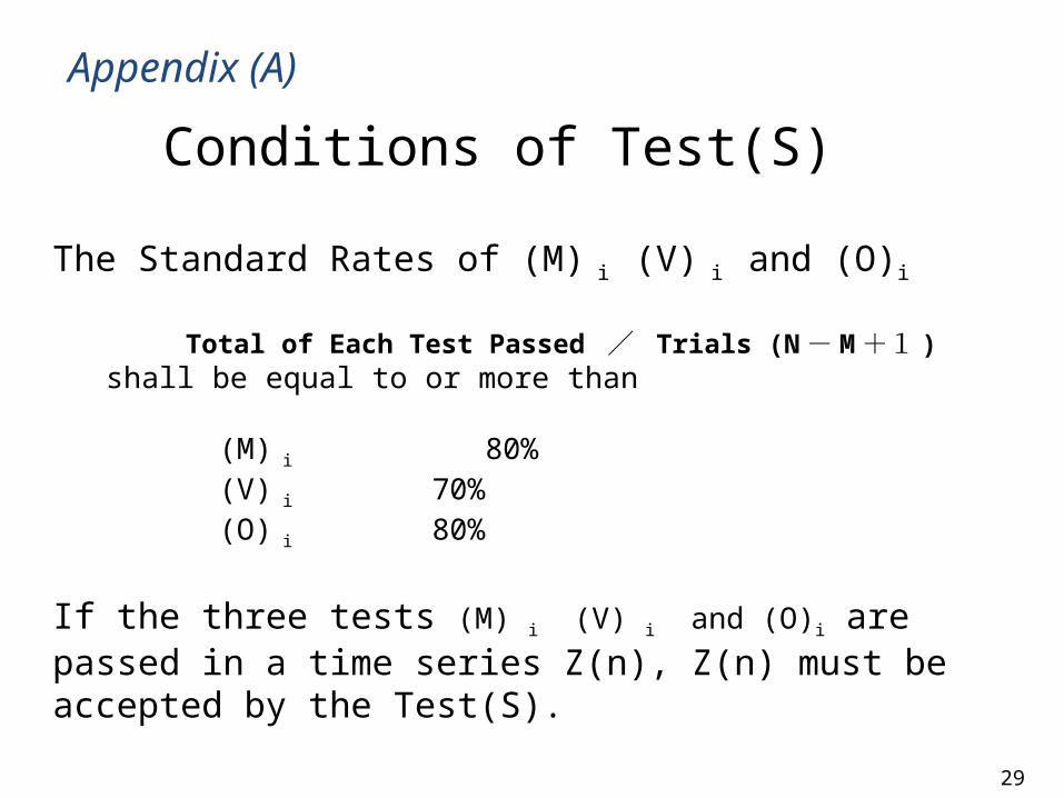
Conditions of Test(S)
29
The Standard Rates of (M) i (V) i and (O)i
Total of Each Test Passed / Trials (N - M +1 ) shall be equal to or more than
1. (M) i 80% 2. (V) i 70%3. (O) i 80%
If the three tests (M) i (V) i and (O)i are passed in a time series Z(n), Z(n) must be accepted by the Test(S).
Appendix (A)
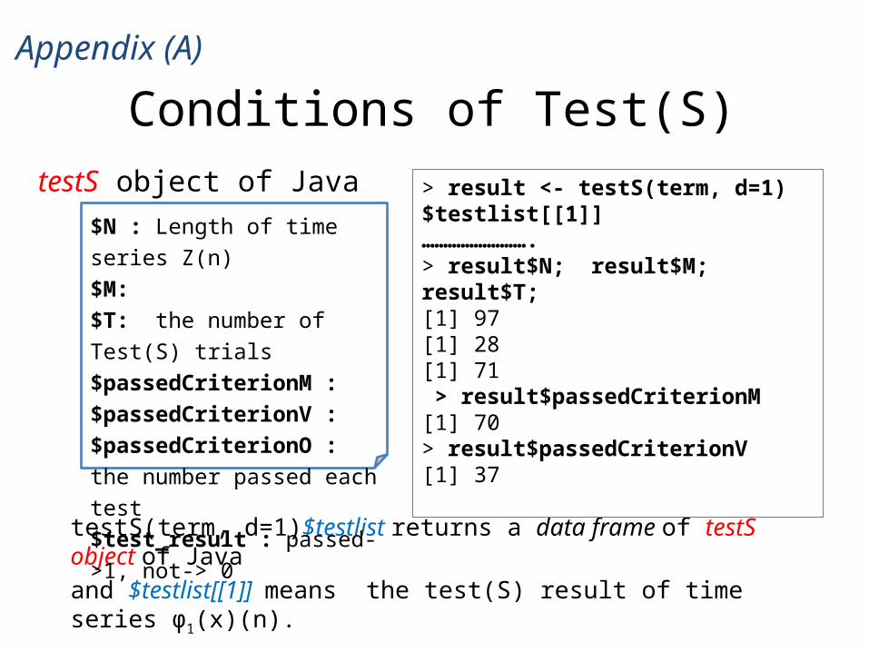
Conditions of Test(S)
• testS(term, d=1)$testlist returns a data frame of testS object of Java • and $testlist[[1]] means the test(S) result of time series φ1(x)(n).
$N : Length of time series Z(n)$M: $T: the number of Test(S) trials$passedCriterionM : $passedCriterionV : $passedCriterionO : the number passed each test$test_result : passed->1, not-> 0
> result <- testS(term, d=1) $testlist[[1]]…………………….> result$N; result$M; result$T;[1] 97[1] 28[1] 71 > result$passedCriterionM[1] 70> result$passedCriterionV[1] 37
testS object of Java
Appendix (A)