Embed Size (px)
Citation preview

Tall-and-skinny Matrix Computations inMapReduce
Austin Benson
Institute for Computational and Mathematical EngineeringStanford University
2nd ICME MapReduce Workshop
April 29, 2013

Collaborators 2
James Demmel, UC-Berkeley David Gleich, Purdue
Paul Constantine, Stanford
Thanks!
Matrices and MapReduce 3
Matrices and MapReduce
Ax
|| · ||
ATA and BTA
QR and SVD
Conclusion

MapReduce overview 4
Two functions that operate on key value pairs:
(key , value)map−−→ (key , value)
(key , 〈value1, . . . , valuen〉)reduce−−−−→ (key , value)
A shuffle stage runs between map and reduce to sort the values bykey.

MapReduce overview 5
Scalability: many map tasks and many reduce tasks are used
https://developers.google.com/appengine/docs/python/images/mapreduce_mapshuffle.png

MapReduce overview 6
The idea is data-local computations. The programmer implements:
I map(key, value)
I reduce(key, 〈 value1, . . ., valuen 〉)
The shuffle and data I/O is implemented by the MapReduceframework, e.g., Hadoop.
This is a very restrictive programming environment! We sacrificeprogram control for structure, scalability, fault tolerance, etc.

MapReduce: control 7
In MapReduce, we cannot control:
I the number of mappers
I which key-value pairs from our data get sent to which mappers
In MapReduce, we can control:
I the number of reducers

Matrix representation 8
We have matrices, so what are the key-value pairs? The key mayjust be a row identifier:
A =
1.0 0.02.4 3.70.8 4.29.0 9.0
→
(1, [1.0, 0.0])(2, [2.4, 3.7])(3, [0.8, 4.2])(4, [9.0, 9.0])
(key, value) → (row index, row)

Matrix representation 9
Maybe the data is a set of samples
A =
1.0 0.02.4 3.70.8 4.29.0 9.0
→
(“Apr 26 04:18:49”, [1.0, 0.0])(“Apr 26 04:18:52”, [2.4, 3.7])(“Apr 26 04:19:12”, [0.8, 4.2])(“Apr 26 04:22:33”, [9.0, 9.0])
(key, value) → (timestamp, sample)

Matrix representation: an example 10
Scientific example: (x, y, z) coordinates and model number:
((47570,103.429767811242,0,-16.525510963787,iDV7), [0.00019924
-4.706066e-05 2.875293979e-05 2.456653e-05 -8.436627e-06 -1.508808e-05
3.731976e-06 -1.048795e-05 5.229153e-06 6.323812e-06])
Figure: Aircraft simulation data. Paul Constantine, Stanford University

Tall-and-skinny matrices 11
What are tall-and-skinny matrices?
A is m × n and m >> n. Examples: rows are data samples; blocksof A are images from a video; Krylov subspaces

Ax 12
Matrices and MapReduce
Ax
|| · ||
ATA and BTA
QR and SVD
Conclusion

Tall-and-skinny matrices 13
Slightly more rigorous definition:It is “cheap” to pass O(n2) data to all processors.

Ax : Local to Distributed 14

Ax : Distributed store, Distributed computation 15
A may be stored in an uneven, distributed fashion. TheMapReduce framework provides load balance.

Ax : MapReduce perspective 16
The programmer’s perspective for map():

Ax : MapReduce implementation 17
1 # x is available locally
2 def map(key, val):
3 yield (key, val * x)

Ax : MapReduce implementation 18
I We didn’t even need reduce!
I The output is stored in distributed fashion:

|| · || 19
Matrices and MapReduce
Ax
|| · ||
ATA and BTA
QR and SVD
Conclusion

||Ax || 20
I Global information → need reduce
I Examples: ||Ax ||1, ||Ax ||2, ||Ax ||∞, |Ax |0

||y ||22 21
Assume we have already computed y = Ax .

||y ||22 22
What can we do with a partial partition of y?

||y ||22 map 23
We could just compute the squares of each
1 def map(key, val):
2 yield (0, val * val)
... then we need to sum the squares

||y ||22 map and reduce 24
Only one key → everything sent to a single reducer.
1 def map(key, val):
2 # only one key
3 yield (0, val * val)
45 def reduce(key, vals):
6 yield (’norm2’, sum(vals))

||y ||22 map and reduce 25
How can this be improved?
1 def map(key, val):
2 # only one key
3 yield (0, val * val)
45 def reduce(key, vals):
6 yield (’norm2’, sum(vals))

||y ||22 improvement 26
Idea: Use more reducers
1 def map1(key , val ) :2 key = uniform random([1 , 2 , 3 , 4 , 5 , 6])3 yield (key , val ∗ val )45 def reduce1(key , vals ) :6 yield (key , sum( vals ))78 def map2(key , val ) :9 yield key , val
1011 def reduce2(key , vals ) :12 yield ( ’norm2 ’ , sum( vals ))
map1() → reduce1() → map2() → reduce2()
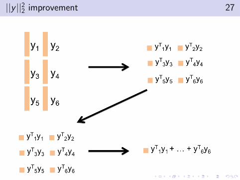
||y ||22 improvement 27

||y ||22 problem 28
I Problem: O(m) data emitted from mappers in first stage.
I Problem: 2 iterations.
I Idea: Do partial summations in the map stage.

||y ||22 improvement 29
1 partial_sum_sq = 0
2 def map(key, val):
3 partial_sum += val * val
4 if key == last_key:
5 yield (0, partial_sum)
67 def reduce(key, vals):
8 yield sum(vals)
I This is the idea of a combiner.
I O(#(mappers)) data emitted from mappers.
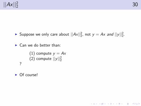
||Ax ||22 30
I Suppose we only care about ||Ax ||22, not y = Ax and ||y ||22.
I Can we do better than:
(1) compute y = Ax(2) compute ||y ||22
?
I Of course!

||Ax ||22 31
Combine our previous ideas:
1 def map(key, val):
2 yield (0, (val * x) * (val * x))
34 def reduce(key, vals):
5 yield sum(vals)

Other norms 32
I We can easily extend these ideas to other norms
I Basic idea for computing ||y ||:
(1) perform some independent operation on each yi(2) combine the results
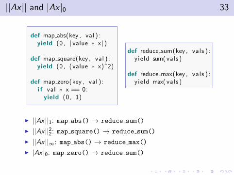
||Ax || and |Ax |0 33
def map abs(key , val ) :yield (0 , | value ∗ x |)
def map square(key , val ) :yield (0 , (value ∗ x)ˆ2)
def map zero(key , val ) :i f val ∗ x == 0:yield (0 , 1)
def reduce sum(key , vals ) :y ie ld sum( vals )
def reduce max(key , vals ) :y ie ld max( vals )
I ||Ax ||1: map abs() → reduce sum()
I ||Ax ||22: map square() → reduce sum()
I ||Ax ||∞: map abs() → reduce max()
I |Ax |0: map zero() → reduce sum()

ATA and BTA 34
Matrices and MapReduce
Ax
|| · ||
ATA and BTA
QR and SVD
Conclusion

ATA 35
We can get a lot from ATA:
I Σ: Singular values
I V T : Right singular vectors
I R from QR

ATA 36
We can get a lot from ATA:
I Σ: Singular values
I V T : Right singular vectors
I R from QR
with a little more work...
I U: Left singular vectors
I Q from QR

ATA: MapReduce 37
I Computing ATA is similar to computing ||y ||22.
I Idea: ATA =m∑i=1
aTi ai (ai is the i-th row).
I → Sum of m n × n rank-1 matrices.
1 def map(key, val):
2 # .T --> Python NumPy transpose
3 yield (0, val.T * val)
45 def reduce(key, vals):
6 yield (0, sum(vals))

ATA: MapReduce 38

ATA: MapReduce 39
I Problem: O(m) matrix sums on a single reducer.
I Idea: have multiple reducers.

ATA: MapReduce 40
I Problem: O(m)#(reducers) matrix sums on a single reducer.
I Problem: need two iterations.

ATA: MapReduce 41
I Need to remove communication of O(m) matrices frommappers to reducers.
I Idea: local partial sums on the mappers.
1 partial_sum = zeros(n, n)
2 def map(key, val):
3 partial_sum += val.T * val
4 if key == last_key:
5 yield (0, partial_sum)
67 def reduce(key, vals):
8 yield (0, sum(vals))
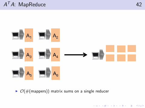
ATA: MapReduce 42
I O(#(mappers)) matrix sums on a single reducer

ATA: MapReduce 43
I Suppose we are willing to have a distributed ATA
I Idea: emit entries of partial sums as values
1 partial_sum = zeros(n, n)
2 def map(key, val):
3 partial_sum += val.T * val
4 if key == last_key:
5 for i = 1:n
6 for j = 1:n
7 yield ((i, j), partial_sum[i, j])
89 def reduce(key, vals):
10 yield (key, sum(vals))

BTA 44
A =
(1, [1.0, 0.0])(2, [2.4, 3.7])(3, [0.8, 4.2])(4, [9.0, 9.0])
, B =
(1, [1.1, 3.2])(2, [9.1, 0.7])(3, [4.3, 2.1])(4, [8.6, 2.1])
I We want to compute BTA =m∑i=1
bTi ai
(bi is i-th row of B, ai is i-th row of A)
I Problem: cannot get ai and bi on the same mapper!

BTA 45
A =
((1,A), [1.0, 0.0])((2,A), [2.4, 3.7])((3,A), [0.8, 4.2])((4,A), [9.0, 9.0])
, B =
((1,B), [1.1, 3.2])((2,B), [9.1, 0.7])((3,B), [4.3, 2.1])((4,B), [8.6, 2.1])
I Idea: In the map stage, use row index as key
I Problem: O(m) rows communicated as data

BTA 46
A =
((1,A), [1.0, 0.0])((2,A), [2.4, 3.7])((3,A), [0.8, 4.2])((4,A), [9.0, 9.0])
, B =
((1,B), [1.1, 3.2])((2,B), [9.1, 0.7])((3,B), [4.3, 2.1])((4,B), [8.6, 2.1])
1 def map(key, val):
2 yield (key[0], (key[1], val))
34 def reduce(key, vals):
5 # We know there are exactly two values
6 (mat_id1, row1) = vals[0]
7 (mat_id2, row2) = vals[1]
8 if mat_id1 == ’A’: yield (rand(), row2.T * row1)
9 else: yield (rand(), row1.T * row2)

BTA 47
I Now we have m rank-1 matrices: bTi ai , i = 1, . . . ,m
I Idea: Use our summation strategies from ATA
1 partial_sum = zeros(n, n)
2 def map(key, val):
3 partial_sum += val.T * val
4 if key == last_key:
5 yield (0, partial_sum)
67 def reduce(key, vals):
8 yield (0, sum(vals))

BTA 48
I Problem: still O(m) rows map → reduce.
I Can’t really get around this problem.
I Result: BTA is much slower than ATA.
QR and SVD 49
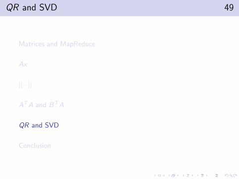
Matrices and MapReduce
Ax
|| · ||
ATA and BTA
QR and SVD
Conclusion

Quick QR and SVD review 50
A Q R
VT
n
n
n
n
n
n
A U n
n
n
n
n
n
Σ
n
n
Figure: Q, U, and V are orthogonal matrices. R is upper triangular andΣ is diagonal with positive entries.
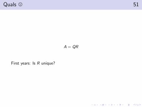
Quals / 51
A = QR
First years: Is R unique?

Tall-and-skinny QR 52
A Q
R
m
n
m
n n
n
Tall-and-skinny (TS): m >> n. QTQ = I .

TS-QR → TS-SVD 53
R is small, so computing its SVD is cheap.

Why Tall-and-skinny QR and SVD? 54
1. Regression with many samples
2. Principle Component Analysis (PCA)
3. Model Reduction
Pressure, Dilation, Jet Engine
Figure: Dynamic mode decomposition of a rectangular supersonicscreeching jet. Joe Nichols, Stanford University.

Cholesky QR 55
Cholesky QR
ATA = (QR)T (QR) = RTQTQR = RTR
Q = AR−1
I We already saw how to compute ATA.
I Compute R = Cholesky(ATA) locally (cheap)
I AR−1 computation is similar to Ax
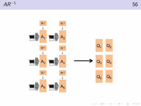
AR−1 56

AR−1 57
1 # R is available locally
2 def map(key, value):
3 yield (key, value * inv(R))
I Problem: Explicitly computing ATA→ unstable
I Idea: ICME Colloquium, 4:15pm May 20, 300/300

Cholesky SVD 58
Q = AR−1
R = URΣV T
A = (QUR)ΣV T = UΣV T
I Compute R = Cholesky(ATA) locally (cheap)
I Compute R = URΣV T locally (cheap)
I U = A(R−1UR) is just an extension of AR−1

A(R−1UR) 59

Conclusion 60
Matrices and MapReduce
Ax
|| · ||
ATA and BTA
QR and SVD
Conclusion

Resources 61
Argh! These are great ideas but I do not want to implement them.
I https://github.com/arbenson/mrtsqr: Matrixcomputations in this talk
I Apache Mahout: machine learning library

Resources 62
Argh! I do not have a MapReduce cluster.
I icme-hadoop1.stanford.edu

Questions 63
Questions?
I https://github.com/arbenson/mrtsqr


![Catalog Icme Ecab[1]](https://img.pdfslide.us/doc/110x75/544c3a1caf7959a4438b59fd/catalog-icme-ecab1.jpg)