Embed Size (px)
Citation preview

Learning objectives
Using Python/SciPy tools:
1 Analyze data using descriptive statistics and graphical tools
2 Fit a probability distribution to data (estimate distribution parameters)
3 Express various risk measures as statistical tests
4 Determine quantile measures of various risk metrics
5 Build flexible models to allow estimation of quantities of interest and associated uncertaintymeasures
6 Select appropriate distributions of random variables/vectors for stochastic phenomena
2 / 75

Where does this fit into risk engineering?
data probabilistic model
event probabilities
consequence model
event consequences
risks
curvefitting
costs
decision-making
criteria
These slides
3 / 75

Where does this fit into risk engineering?
data probabilistic model
event probabilities
consequence model
event consequences
risks
curvefitting
costs
decision-making
criteria
These slides
3 / 75

Where does this fit into risk engineering?
data probabilistic model
event probabilities
consequence model
event consequences
risks
curvefitting
costs
decision-making
criteria
These slides
3 / 75
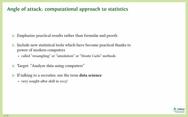
Angle of attack: computational approach to statistics
▷ Emphasize practical results rather than formulæ and proofs
▷ Include new statistical tools which have become practical thanks topower of modern computers• called “resampling” or “simulation” or “Monte Carlo” methods
▷ Target: “Analyze data using computers”
▷ If talking to a recruiter, use the term data science• very sought-after skill in 2015!
4 / 75

Python and SciPy
Environment used in this coursework:
▷ Python programming language + SciPy + NumPy + matplotlib libraries
▷ Alternative to Matlab, Scilab, Octave, R
▷ free software
▷ a real programming language with simple syntax
▷ rich scientific computing libraries• statistical measures
• visual presentation of data
• optimization, interpolation and curve fitting
• stochastic simulation
• machine learning, image processing…
5 / 75

Installation options
▷ Microsoft Windows: install one of• Anaconda from http://continuum.io/downloads
• pythonxy from http://code.google.com/p/pythonxy/
▷ MacOS: install one of• Anaconda from http://continuum.io/downloads
• Pyzo, from http://www.pyzo.org/
▷ Linux: install packages python, numpy, matplotlib, scipy• your distribution’s packages are probably fine
▷ Cloud without local installation: Sage Math Cloud• IPython and Sage running in the cloud
6 / 75

Sage Math Cloud
▷ Runs in cloud, access viabrowser
▷ No local installation needed
▷ Access to IPython, Sage, R
▷ Create an account for free
▷ cloud.sagemath.com
▷ Similar:pythonanywhere.com
7 / 75
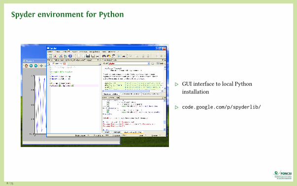
Spyder environment for Python
▷ GUI interface to local Pythoninstallation
▷ code.google.com/p/spyderlib/
8 / 75

Python: interactive work in a console
▷ IPython notebook: interact via your web browser
▷ Type expressions into a cell then press Ctrl-Enter
▷ Results appear in the web page
9 / 75

Python: loading a program from a script
▷ For more complex problems, write a program into a file
▷ Load the program using implementation’s Load facility
10 / 75
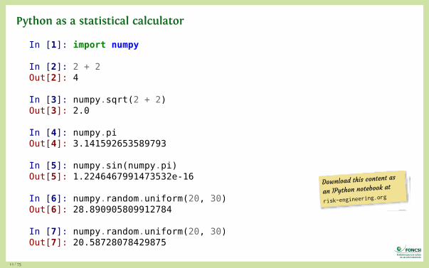
Python as a statistical calculator
In [1]: import numpy
In [2]: 2 + 2Out[2]: 4
In [3]: numpy.sqrt(2 + 2)Out[3]: 2.0
In [4]: numpy.piOut[4]: 3.141592653589793
In [5]: numpy.sin(numpy.pi)Out[5]: 1.2246467991473532e-16
In [6]: numpy.random.uniform(20, 30)Out[6]: 28.890905809912784
In [7]: numpy.random.uniform(20, 30)Out[7]: 20.58728078429875
D o w n l o a dt h i s c o n t e n
t a s
a n I P y t h o nn o t e b o o k a
t
risk-engineering.org
11 / 75
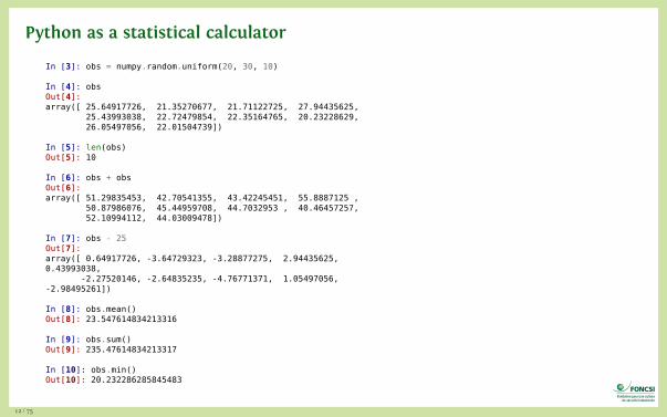
Python as a statistical calculator
In [3]: obs = numpy.random.uniform(20, 30, 10)
In [4]: obsOut[4]:array([ 25.64917726, 21.35270677, 21.71122725, 27.94435625,
25.43993038, 22.72479854, 22.35164765, 20.23228629,26.05497056, 22.01504739])
In [5]: len(obs)Out[5]: 10
In [6]: obs + obsOut[6]:array([ 51.29835453, 42.70541355, 43.42245451, 55.8887125 ,
50.87986076, 45.44959708, 44.7032953 , 40.46457257,52.10994112, 44.03009478])
In [7]: obs - 25Out[7]:array([ 0.64917726, -3.64729323, -3.28877275, 2.94435625,0.43993038,
-2.27520146, -2.64835235, -4.76771371, 1.05497056,-2.98495261])
In [8]: obs.mean()Out[8]: 23.547614834213316
In [9]: obs.sum()Out[9]: 235.47614834213317
In [10]: obs.min()Out[10]: 20.232286285845483
12 / 75

Python as a statistical calculator: plotting
In [2]: import numpy, matplotlib.pyplot as plt
In [3]: x = numpy.linspace(0, 10, 100)
In [4]: obs = numpy.sin(x) + numpy.random.uniform(-0.1, 0.1, 100)
In [5]: plt.plot(x, obs)
In [7]: plt.plot(x, obs)
Out[5]: [<matplotlib.lines.Line2D at 0x7f47ecc96da0>]
Out[7]: [<matplotlib.lines.Line2D at 0x7f47ed42f0f0>]
13 / 75

Coming from Matlab
Generate random numbers
MATLAB/Octave Python Description
rand(1,10) random.random((10,))
random.uniform((10,))
Uniform distribution
2+5*rand(1,10) random.uniform(2,7,(10,)) Uniform: Numbers between 2and 7
rand(6) random.uniform(0,1,(6,6)) Uniform: 6,6 array
randn(1,10) random.standard_normal((10,)) Normal distribution
Vectors
MATLAB/Octave Python Description
a=[2 3 4 5]; a=array([2,3,4,5]) Row vector, $1 \times n$ matrix
Source: http://mathesaurus.sourceforge.net/matlab-numpy.html
14 / 75
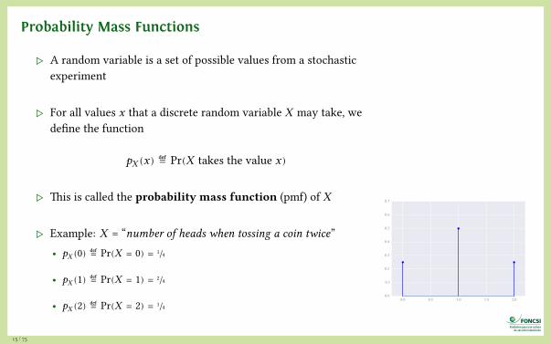
Probability Mass Functions
▷ A random variable is a set of possible values from a stochasticexperiment
▷ For all values x that a discrete random variable X may take, wedefine the function
pX (x) ≝ Pr(X takes the value x)
▷ This is called the probability mass function (pmf) of X
▷ Example: X = “number of heads when tossing a coin twice”• pX (0) ≝ Pr(X = 0) = 1/4
• pX (1) ≝ Pr(X = 1) = 2/4
• pX (2) ≝ Pr(X = 2) = 1/40.0 0.5 1.0 1.5 2.0
0.0
0.1
0.2
0.3
0.4
0.5
0.6
0.7
15 / 75

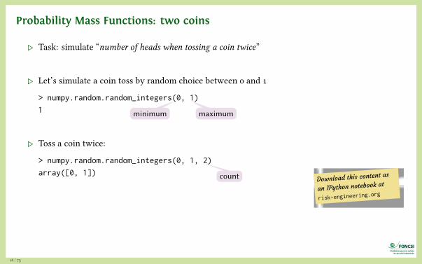
Probability Mass Functions: two coins
▷ Task: simulate “number of heads when tossing a coin twice”
▷ Let’s simulate a coin toss by random choice between 0 and 1
> numpy.random.random_integers(0, 1)
1
▷ Toss a coin twice:
> numpy.random.random_integers(0, 1, 2)
array([0, 1])
▷ Number of heads when tossing a coin twice:
> numpy.random.random_integers(0, 1, 2).sum()
1
minimum maximum
D o w n l o a dt h i s c o n t e n
t a s
a n I P y t h o nn o t e b o o k a
t
risk-engineering.org
16 / 75
Probability Mass Functions: two coins
▷ Task: simulate “number of heads when tossing a coin twice”
▷ Let’s simulate a coin toss by random choice between 0 and 1
> numpy.random.random_integers(0, 1)
1
▷ Toss a coin twice:
> numpy.random.random_integers(0, 1, 2)
array([0, 1])
▷ Number of heads when tossing a coin twice:
> numpy.random.random_integers(0, 1, 2).sum()
1
minimum maximum
countD o w n l o a d
t h i s c o n t e nt a s
a n I P y t h o nn o t e b o o k a
t
risk-engineering.org
16 / 75

Probability Mass Functions: two coins
▷ Task: simulate “number of heads when tossing a coin twice”
▷ Do this 1000 times and plot the resulting PMF:
1 import matplotlib.pyplot as plt
2 N = 1000
3 heads = numpy.zeros(N, dtype=int)
4 for i in range(N):
5 heads[i] = numpy.random.random_integers(0, 1, 2).sum()
6 plt.stem(numpy.bincount(heads), marker=’o’)
7 plt.margins(0.1)
heads[i]: e l e m en t n u m b e r
i
o f t h e a r r ay heads
17 / 75

More information on Python programming
▷ For more information on Python syntax, check out thebook Think Python
▷ Purchase, or read online for free atgreenteapress.com/thinkpython
18 / 75
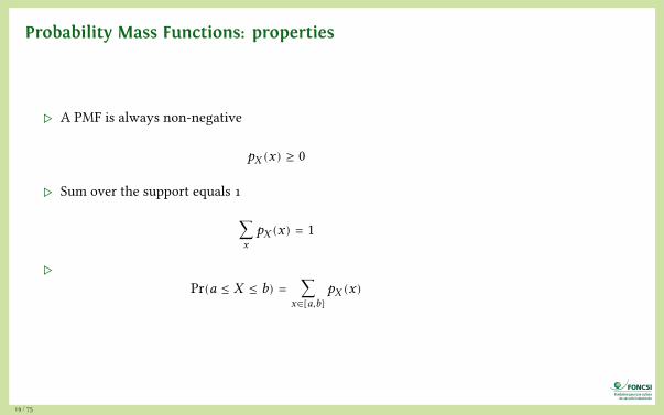
Probability Mass Functions: properties
▷ A PMF is always non-negative
pX (x) ≥ 0
▷ Sum over the support equals 1
∑xpX (x) = 1
▷Pr(a ≤ X ≤ b) = ∑
x∈[a,b]pX (x)
19 / 75

Probability Density Functions
▷ For continuous random variables, the probability densityfunction fX (x) is defined by
Pr(a ≤ X ≤ b) = ∫b
afX (x)dx
▷ It is non-negative
fX (x) ≥ 0
▷ The integral over ℝ is 1
∫∞
−∞fX (x)dx = 1
20 / 75
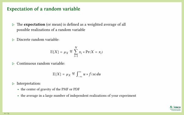
Expectation of a random variable
▷ The expectation (or mean) is defined as a weighted average of allpossible realizations of a random variable
▷ Discrete random variable:
𝔼[X ] = 𝜇X ≝N∑i=1
xi × Pr(X = xi)
▷ Continuous random variable:
𝔼[X ] = 𝜇X ≝ ∫∞
−∞u × f (u)du
▷ Interpretation:• the center of gravity of the PMF or PDF
• the average in a large number of independent realizations of your experiment
21 / 75

Illustration: expected value with coins
▷ X = “number of heads when tossing a coin twice”
▷ PMF:• pX (0) ≝ Pr(X = 0) = 1/4
• pX (1) ≝ Pr(X = 1) = 2/4
• pX (2) ≝ Pr(X = 2) = 1/4
▷ 𝔼[X ] ≝ ∑kk × pX (k) = 0 ×
14
+ 1 ×24
+ 2 ×14
= 1
HH
T
TH
T
22 / 75

Illustration: expected value of a dice roll
▷ Expected value of a dice roll is6
∑i=1
i ×16= 3.5
▷ If we toss a dice a large number of times, the mean value shouldconverge to 3.5
▷ Let’s check that in Python
1 N = 1000
2 roll = numpy.zeros(N)
3 expectation = numpy.zeros(N)
4 for i in range(N):
5 roll[i] = numpy.random.random_integers(1, 6)
6 for i in range(1, N):
7 expectation[i] = numpy.mean(roll[0:i])
8 plt.plot(expectation)0 200 400 600 800 1000
Number of rolls
0
1
2
3
4
5
6
Expe
cted
val
ue
Expectation of a dice roll
23 / 75

Mathematical properties of expectation
If c is a constant and X and Y are random variables, then
▷ 𝔼[c] = c
▷ 𝔼[cX ] = c𝔼[X ]
▷ 𝔼[c + X ] = c + 𝔼[X ]
▷ 𝔼[X + Y ] = 𝔼[X ] + 𝔼[Y ]
Note: in general 𝔼[g(X )] ≠ g(𝔼[X ])
24 / 75
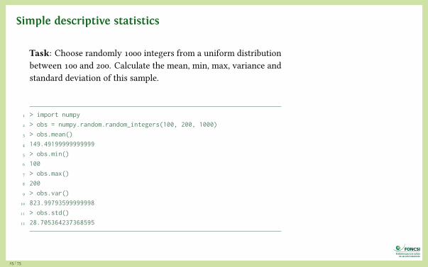
Simple descriptive statistics
Task: Choose randomly 1000 integers from a uniform distributionbetween 100 and 200. Calculate the mean, min, max, variance andstandard deviation of this sample.
1 > import numpy
2 > obs = numpy.random.random_integers(100, 200, 1000)
3 > obs.mean()
4 149.49199999999999
5 > obs.min()
6 100
7 > obs.max()
8 200
9 > obs.var()
10 823.99793599999998
11 > obs.std()
12 28.705364237368595
25 / 75
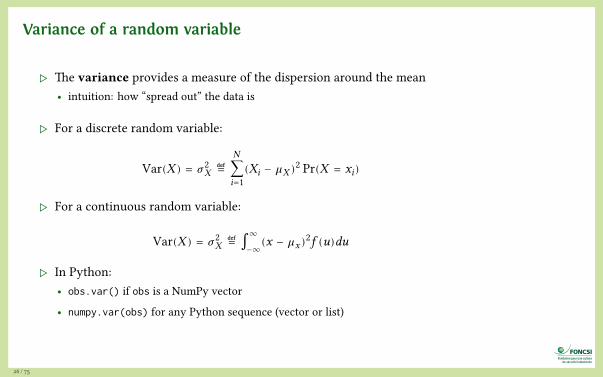
Variance of a random variable
▷ The variance provides a measure of the dispersion around the mean• intuition: how “spread out” the data is
▷ For a discrete random variable:
Var(X ) = 𝜎2X ≝
N∑i=1
(Xi − 𝜇X )2 Pr(X = xi)
▷ For a continuous random variable:
Var(X ) = 𝜎2X ≝ ∫
∞
−∞(x − 𝜇x)2f (u)du
▷ In Python:• obs.var() if obs is a NumPy vector
• numpy.var(obs) for any Python sequence (vector or list)
26 / 75

Variance with coins
▷ X = “number of heads when tossing a coin twice”
▷ PMF:• pX (0) ≝ Pr(X = 0) = 1/4
• pX (1) ≝ Pr(X = 1) = 2/4
• pX (2) ≝ Pr(X = 2) = 1/4
▷
Var(X ) ≝N∑i=1
(Xi − 𝜇X )2 Pr(X = xi)
=14
× (0 − 1)2 +24
× (1 − 1)2 +14
× (2 − 1)2 =12
27 / 75

Variance of a dice roll
▷ Analytic calculation of the variance of a dice roll:
Var(X ) ≝N∑i=1
(Xi − 𝜇X )2 Pr(X = xi)
=16
× ((1 − 3.5)2 + (2 − 3.5)2 + (3 − 3.5)2 + (4 − 4.5)2 + (5 − 3.5)2 + (6 − 3.5)2)
= 2.916
▷ Let’s reproduce that in Python
> rolls = numpy.random.random_integers(1, 6, 1000)
> len(rolls)
1000
> rolls.var()
2.9463190000000004
count
28 / 75
Properties of variance as a mathematical operator
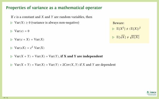
If c is a constant and X and Y are random variables, then
▷ Var(X ) ≥ 0 (variance is always non-negative)
▷ Var(c) = 0
▷ Var(c + X ) = Var(X )
▷ Var(cX ) = c2 Var(X )
▷ Var(X + Y ) = Var(X ) + Var(Y ), if X and Y are independent
▷ Var(X + Y ) = Var(X ) + Var(Y ) + 2Cov(X , Y ) if X and Y are dependent
Note:
▷ Cov(X , Y ) ≝ 𝔼 [(X − 𝔼[X ])(Y − 𝔼[Y ])]
▷ Cov(X ,X ) = Var(X )
29 / 75
Beware:
▷ 𝔼[X 2] ≠ (𝔼[X ])2
▷ 𝔼[√X ] ≠ √𝔼[X ]

Properties of variance as a mathematical operator
If c is a constant and X and Y are random variables, then
▷ Var(X ) ≥ 0 (variance is always non-negative)
▷ Var(c) = 0
▷ Var(c + X ) = Var(X )
▷ Var(cX ) = c2 Var(X )
▷ Var(X + Y ) = Var(X ) + Var(Y ), if X and Y are independent
▷ Var(X + Y ) = Var(X ) + Var(Y ) + 2Cov(X , Y ) if X and Y are dependent
Note:
▷ Cov(X , Y ) ≝ 𝔼 [(X − 𝔼[X ])(Y − 𝔼[Y ])]
▷ Cov(X ,X ) = Var(X )
29 / 75
Beware:
▷ 𝔼[X 2] ≠ (𝔼[X ])2
▷ 𝔼[√X ] ≠ √𝔼[X ]
Standard deviation
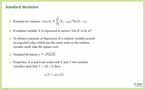
▷ Formula for variance: Var(X ) ≝N∑i=1
(Xi − 𝜇X )2 Pr(X = xi)
▷ If random variable X is expressed in metres, Var(X ) is in m2
▷ To obtain a measure of dispersion of a random variable aroundits expected value which has the same units as the randomvariable itself, take the square root
▷ Standard deviation 𝜎 ≝ √Var(X )
▷ Properties: if a and b are scalar and X and Y two randomvariables such that Y = aX + b, then
𝜎(Y ) = |a| 𝜎(X )
30 / 75

Properties of expectation & variance: empirical testing with numpy
▷ 𝔼[X + Y ] = 𝔼[X ] + 𝔼[Y ]
1 > X = numpy.random.random_integers(1, 100, 1000)
2 > Y = numpy.random.random_integers(-300, -200, 1000)
3 > X.mean()
4 50.575000000000003
5 > Y.mean()
6 -251.613
7 > (X + Y).mean()
8 -201.038
▷ Var(cX ) = c2 Var(X )
1 > numpy.random.random_integers(1, 100, 1000).var()
2 836.616716
3 > numpy.random.random_integers(5, 500, 1000).var()
4 20514.814318999997
5 > 5 * 5 * 836
6 20900
31 / 75
Properties of expectation & variance: empirical testing with numpy
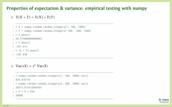
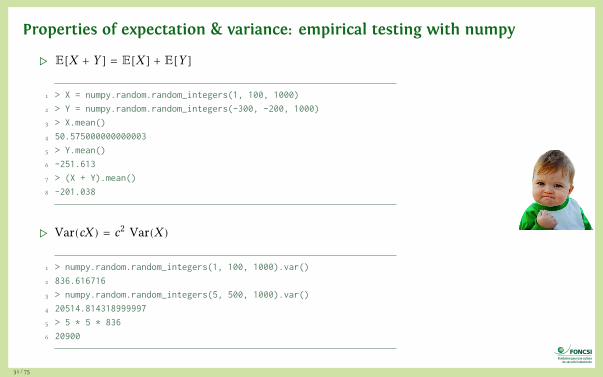
▷ 𝔼[X + Y ] = 𝔼[X ] + 𝔼[Y ]
1 > X = numpy.random.random_integers(1, 100, 1000)
2 > Y = numpy.random.random_integers(-300, -200, 1000)
3 > X.mean()
4 50.575000000000003
5 > Y.mean()
6 -251.613
7 > (X + Y).mean()
8 -201.038
▷ Var(cX ) = c2 Var(X )
1 > numpy.random.random_integers(1, 100, 1000).var()
2 836.616716
3 > numpy.random.random_integers(5, 500, 1000).var()
4 20514.814318999997
5 > 5 * 5 * 836
6 20900
31 / 75

Cumulative Distribution Function
▷ The cumulative distribution function (CDF) of random variable X ,denoted by F (x), indicates the probability that X assumes a value ≤ x ,where x is any real number
F (x) = Pr(X ≤ x) − ∞ ≤ x ≤ ∞
▷ Properties of a CDF:• F (x) is a non-decreasing function of x
• 0 ≤ F (x) ≤ 1
• limx→∞ F (x) = 1
• limx→∞ F (x) = 0
• if x ≤ y then F (x) ≤ F (y)
• Pr(a < X ≤ b) = F (b) − F (a) ∀b > a
32 / 75

CDF of a discrete distribution
F (x) = Pr(X ≤ x) − ∞ ≤ x ≤ ∞
= ∑xi≤x
Pr(X = xi)
Example: sum of two dice
0 2 4 6 8 10 120.00
0.02
0.04
0.06
0.08
0.10
0.12
0.14
0.16
0.18 Sum of two dice: PDF
0 2 4 6 8 10 120.0
0.2
0.4
0.6
0.8
1.0 Sum of two dice: CDF
33 / 75

Scipy.stats package
▷ The scipy.stats module implements manycontinuous and discrete random variables and theirassociated distributions• binomial, poisson, exponential, normal, uniform,weibull…
▷ Usage: instantiate a distribution then call a method• rvs: random variates
• pdf: Probability Density Function
• cdf: Cumulative Distribution Function
• sf: Survival Function (1-CDF)
• ppf: Percent Point Function (inverse of CDF)
• isf: Inverse Survival Function (inverse of SF)
34 / 75
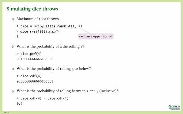
Simulating dice throws
▷ Maximum of 1000 throws
> dice = scipy.stats.randint(1, 7)
> dice.rvs(1000).max()
6
▷ What is the probability of a die rolling 4?
> dice.pmf(4)
0.16666666666666666
▷ What is the probability of rolling 4 or below?
> dice.cdf(4)
0.66666666666666663
▷ What is the probability of rolling between 2 and 4 (inclusive)?
> dice.cdf(4) - dice.cdf(1)
0.5
exclusive upper bound
35 / 75

Simulating dice
1 > import numpy
2 > import matplotlib.pyplot as plt
3 > tosses = numpy.random.choice(range(1, 7))
4 > tosses
5 2
6 > tosses = numpy.random.choice(range(1, 7), 10000)
7 > tosses
8 array([6, 6, 4, ..., 2, 4, 5])
9 > tosses.mean()
10 3.4815
11 > numpy.median(tosses)
12 3.0
13 > len(numpy.where(tosses > 3)[0])
14 4951
15 > plt.hist(tosses, bins=6)
1 2 3 4 5 6 70
200
400
600
800
1000
1200
1400
1600
1800
36 / 75
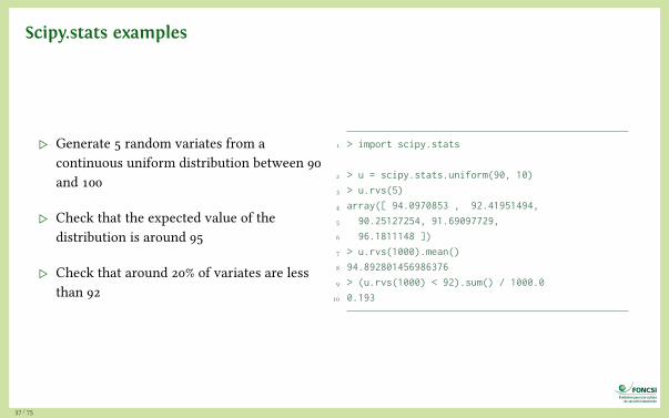
Scipy.stats examples
▷ Generate 5 random variates from acontinuous uniform distribution between 90and 100
▷ Check that the expected value of thedistribution is around 95
▷ Check that around 20% of variates are lessthan 92
1 > import scipy.stats
2 > u = scipy.stats.uniform(90, 10)
3 > u.rvs(5)
4 array([ 94.0970853 , 92.41951494,
5 90.25127254, 91.69097729,
6 96.1811148 ])
7 > u.rvs(1000).mean()
8 94.892801456986376
9 > (u.rvs(1000) < 92).sum() / 1000.0
10 0.193
37 / 75
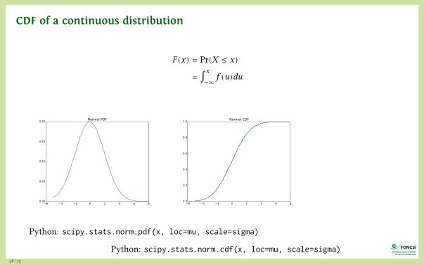
CDF of a continuous distribution
F (x) = Pr(X ≤ x)
= ∫x
−∞f (u)du
6 4 2 0 2 4 6 80.00
0.05
0.10
0.15
0.20 Normal PDF
6 4 2 0 2 4 6 80.0
0.2
0.4
0.6
0.8
1.0 Normal CDF
Python: scipy.stats.norm.pdf(x, loc=mu, scale=sigma)
Python: scipy.stats.norm.cdf(x, loc=mu, scale=sigma)38 / 75

Some
important
probability
distributions
39 / 75
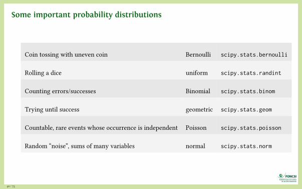
Some important probability distributions
Coin tossing with uneven coin Bernoulli scipy.stats.bernoulli
Rolling a dice uniform scipy.stats.randint
Counting errors/successes Binomial scipy.stats.binom
Trying until success geometric scipy.stats.geom
Countable, rare events whose occurrence is independent Poisson scipy.stats.poisson
Random “noise”, sums of many variables normal scipy.stats.norm
40 / 75

Bernoulli trials
▷ A trial is an experiment which can be repeated many times withthe same probabilities, each realization being independent of theothers
▷ Bernoulli trial: an experiment in which N trials are made of anevent, with probability p of “success” in any given trial andprobability 1 − p of “failure”• “success” and “failure” are mutually exclusive
• example: sequence of coin tosses
• example: arrival of requests in a web server per time slot
Jakob Bernoulli (1654–1705)
41 / 75

The geometric distribution (trying until success)
▷ We conduct a sequence of Bernoulli trials, each with successprobability p
▷ What’s the probability that it takes k trials to get a success?• Before we can succeed at trial k, we must have had k − 1 failures
• Each failure occurred with probability 1 − p, so total probability(1 − p)k−1
• Then a single success with probability p
▷ Pr(X = k) = (1 − p)k−1p
0 2 4 6 8 10 12 140.00
0.05
0.10
0.15
0.20
0.25
0.30 Geometric distribution PMF, p=0.3
42 / 75
The geometric distribution: intuition
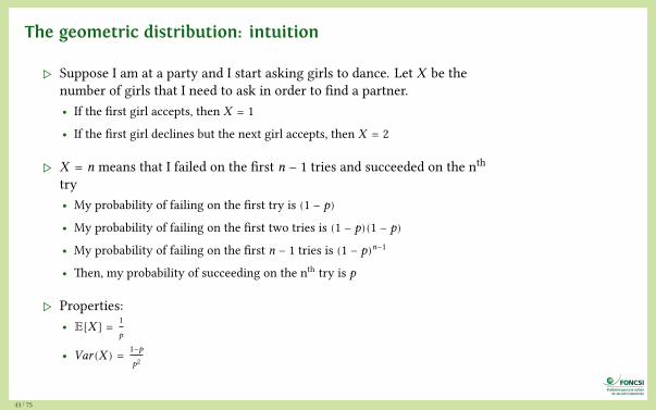
▷ Suppose I am at a party and I start asking girls to dance. Let X be thenumber of girls that I need to ask in order to find a partner.• If the first girl accepts, then X = 1
• If the first girl declines but the next girl accepts, then X = 2
▷ X = n means that I failed on the first n − 1 tries and succeeded on the nth
try• My probability of failing on the first try is (1 − p)
• My probability of failing on the first two tries is (1 − p)(1 − p)
• My probability of failing on the first n − 1 tries is (1 − p)n−1
• Then, my probability of succeeding on the nth try is p
▷ Properties:• 𝔼[X ] =
1
p
• Var(X ) =1−p
p2
43 / 75

The binomial distribution (counting successes)
▷ Also arises when observing multiple Bernoulli trials• exactly two mutually exclusive outcomes, “success” and “failure”
▷ Binomial(p, k, n): the probability of observing k successes in ntrials, with the probability of success on a single trial denoted byp• example: toss a coin n times (p = 0.5) and see k heads
▷ We have k successes, which happens with a probability of pk
▷ We have n − k failures, which happens with probability(1 − p)n−k
▷ We can generate these k successes in many different ways fromn trials, (nk) ways
▷ Pr(X = k) = (nk)(1 − p)n−kpk
0 5 10 15 200.00
0.05
0.10
0.15
0.20 Binomial distribution PMF, n=20, p=0.3
44 / 75
Reminder: binomialcoefficient (n
k) is n!
k!(n−k)!

Binomial distribution: application
▷ Consider a medical test with an error rate of0.1 applied to 100 patients
▷ What is the probability that we see at most 1test error?
▷ What is the probability that we see at most10 errors?
▷ What is the smallest k such that P(X ≤ k) isat least 0.05?
1 > import scipy.stats
2 > test = scipy.stats.binom(n=100, p=0.1)
3 > test.cdf(1)
4 0.00032168805319411544
5 > test.cdf(10)
6 0.58315551226649232
7 > test.ppf(0.05)
8 5.0
45 / 75

Binomial distribution: application
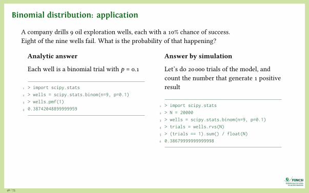
A company drills 9 oil exploration wells, each with a 10% chance of success.Eight of the nine wells fail. What is the probability of that happening?
Analytic answer
Each well is a binomial trial with p = 0.1
1 > import scipy.stats
2 > wells = scipy.stats.binom(n=9, p=0.1)
3 > wells.pmf(1)
4 0.38742048899999959
Answer by simulation
Let’s do 20 000 trials of the model, andcount the number that generate 1 positiveresult
1 > import scipy.stats
2 > N = 20000
3 > wells = scipy.stats.binom(n=9, p=0.1)
4 > trials = wells.rvs(N)
5 > (trials == 1).sum() / float(N)
6 0.38679999999999998
The probability of all 9 wells failing is 0.99 = 0.3874 (and also wells.pmf(0)).The probability of at least 8 wells failing is wells.cdf(1). It’s alsowells.pmf(0) + wells.pmf(1) (it’s 0.7748).
46 / 75
Binomial distribution: application
A company drills 9 oil exploration wells, each with a 10% chance of success.Eight of the nine wells fail. What is the probability of that happening?
Analytic answer
Each well is a binomial trial with p = 0.1
1 > import scipy.stats
2 > wells = scipy.stats.binom(n=9, p=0.1)
3 > wells.pmf(1)
4 0.38742048899999959
Answer by simulation
Let’s do 20 000 trials of the model, andcount the number that generate 1 positiveresult
1 > import scipy.stats
2 > N = 20000
3 > wells = scipy.stats.binom(n=9, p=0.1)
4 > trials = wells.rvs(N)
5 > (trials == 1).sum() / float(N)
6 0.38679999999999998
The probability of all 9 wells failing is 0.99 = 0.3874 (and also wells.pmf(0)).The probability of at least 8 wells failing is wells.cdf(1). It’s alsowells.pmf(0) + wells.pmf(1) (it’s 0.7748).
46 / 75
Binomial distribution: properties
Exercise: check empirically (with SciPy) the following propertiesof the binomial distribution:
▷ the mean of the distribution (𝜇x ) is equal to n × p
▷ the variance (𝜎2X ) is n × p × (1 − p)
▷ the standard deviation (𝜎x ) is √n × p × (1 − p)
47 / 75

Gaussian (normal) distribution
▷ The famous “bell shaped” curve, fully described by its mean andstandard deviation
▷ Good representation of distribution of measurement errors andmany population characteristics• size, mechanical strength, duration, speed
▷ Symmetric around the mean
▷ Mean = median = mode
6 4 2 0 2 4 6 80.00
0.05
0.10
0.15
0.20 Normal PDF
48 / 75
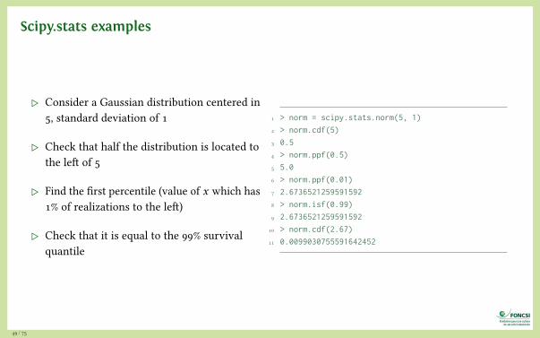
Scipy.stats examples
▷ Consider a Gaussian distribution centered in5, standard deviation of 1
▷ Check that half the distribution is located tothe left of 5
▷ Find the first percentile (value of x which has1% of realizations to the left)
▷ Check that it is equal to the 99% survivalquantile
1 > norm = scipy.stats.norm(5, 1)
2 > norm.cdf(5)
3 0.5
4 > norm.ppf(0.5)
5 5.0
6 > norm.ppf(0.01)
7 2.6736521259591592
8 > norm.isf(0.99)
9 2.6736521259591592
10 > norm.cdf(2.67)
11 0.0099030755591642452
49 / 75

Area under the normal distribution
In [1]: import numpy
In [2]: from scipy.stats import norm
In [3]: norm.ppf(0.5)Out[3]: 0.0
In [4]: norm.cdf(0)Out[4]: 0.5
In [5]: norm.cdf(2) - norm.cdf(-2)Out[5]: 0.95449973610364158
In [6]: norm.cdf(3) - norm.cdf(-3)Out[6]: 0.99730020393673979
quantile function
there is a 95% chance that the number drawn falls within2 standard deviations of the mean
−4 −3 −2 −1 0 1 2 3 40.00
0.05
0.10
0.15
0.20
0.25
0.30
0.35
0.40
−4 −3 −2 −1 0 1 2 3 40.00
0.05
0.10
0.15
0.20
0.25
0.30
0.35
0.40
I n p r e h i s t or i c t i m e s ,
s t a t i s t i c s te x t b o o k s c
o n t a i n e d la r g e t a b l e
s
o f d i f f e r e nt q u a n t i l e
v a l u e s o f th e n o r m a l
d i s t r i b u t i on . W i t h
c h e a p c o mp u t i n g p o w
e r , n o l o n ge r n e c e s s a
r y !
50 / 75
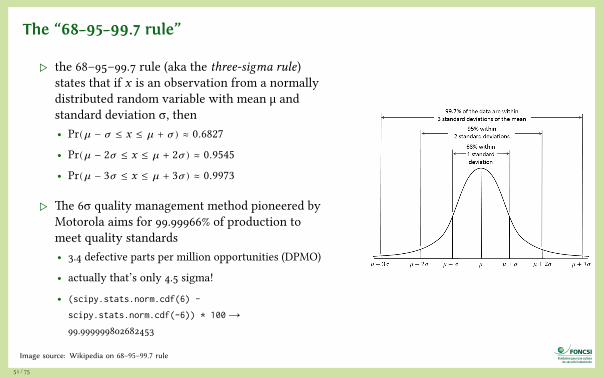
The “68–95–99.7 rule”
▷ the 68–95–99.7 rule (aka the three-sigma rule)states that if x is an observation from a normallydistributed random variable with mean μ andstandard deviation σ, then• Pr(u� − u� ≤ x ≤ u� + u�) ≈ 0.6827
• Pr(u� − 2u� ≤ x ≤ u� + 2u�) ≈ 0.9545
• Pr(u� − 3u� ≤ x ≤ u� + 3u�) ≈ 0.9973
▷ The 6σ quality management method pioneered byMotorola aims for 99.99966% of production tomeet quality standards• 3.4 defective parts per million opportunities (DPMO)
• actually that’s only 4.5 sigma!
• (scipy.stats.norm.cdf(6) -
scipy.stats.norm.cdf(-6)) * 100 →99.999999802682453
Image source: Wikipedia on 68–95–99.7 rule
51 / 75
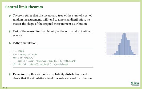
Central limit theorem
▷ Theorem states that the mean (also true of the sum) of a set ofrandom measurements will tend to a normal distribution, nomatter the shape of the original measurement distribution
▷ Part of the reason for the ubiquity of the normal distribution inscience
▷ Python simulation:
1 N = 10000
2 sim = numpy.zeros(N)
3 for i in range(N):
4 sim[i] = numpy.random.uniform(30, 40, 100).mean()
5 plt.hist(sim, bins=20, alpha=0.5, normed=True)
▷ Exercise: try this with other probability distributions andcheck that the simulations tend towards a normal distribution
34.6 34.7 34.8 34.9 35.0 35.1 35.2 35.30.0
0.5
1.0
1.5
2.0
2.5
3.0
3.5
4.0
4.5
52 / 75
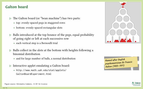
Galton board
▷ The Galton board (or “bean machine”) has two parts:• top: evenly-spaced pegs in staggered rows
• bottom: evenly-spaced rectangular slots
▷ Balls introduced at the top bounce of the pegs, equal probabilityof going right or left at each successive row• each vertical step is a Bernoulli trial
▷ Balls collect in the slots at the bottom with heights following abinomial distribution• and for large number of balls, a normal distribution
▷ Interactive applet emulating a Galton board:• http://www.math.uah.edu/stat/applets/
GaltonBoardExperiment.html
Figure source: Wikimedia Commons, CC BY-SA licence
N a m e d a f te r E n g l i s h
p s y c h o m e tr i c i a n S i r F
r a n c i s
G a l t o n ( 1 82 2 – 1 9 1 1 )
53 / 75
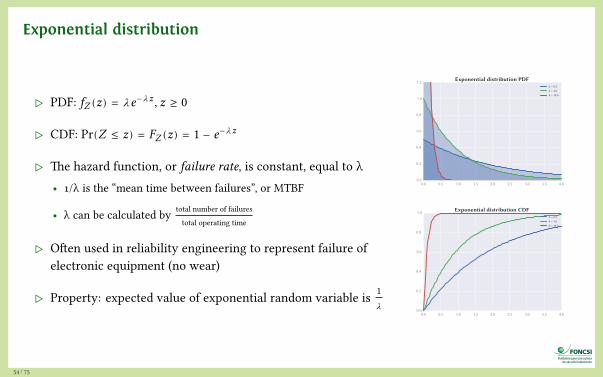
Exponential distribution
▷ PDF: fZ (z) = 𝜆e−u�z , z ≥ 0
▷ CDF: Pr(Z ≤ z) = FZ (z) = 1 − e−u�z
▷ The hazard function, or failure rate, is constant, equal to λ• 1/λ is the “mean time between failures”, or MTBF
• λ can be calculated by total number of failures
total operating time
▷ Often used in reliability engineering to represent failure ofelectronic equipment (no wear)
▷ Property: expected value of exponential random variable is 1u�
0.0 0.5 1.0 1.5 2.0 2.5 3.0 3.5 4.00.0
0.2
0.4
0.6
0.8
1.0
1.2 Exponential distribution PDFλ = 0.5λ = 1.0λ = 10.0
0.0 0.5 1.0 1.5 2.0 2.5 3.0 3.5 4.00.0
0.2
0.4
0.6
0.8
1.0 Exponential distribution CDFλ = 0.5λ = 1.0λ = 10.0
54 / 75
Exponential distribution
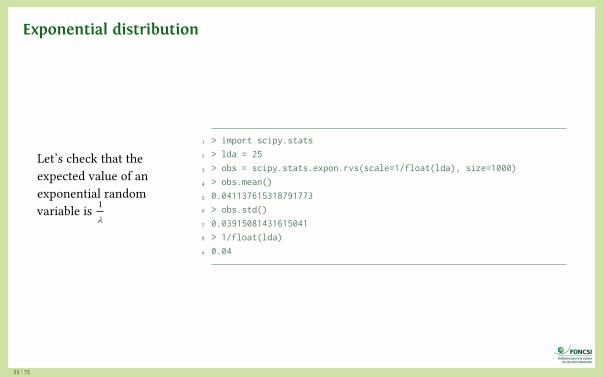
Let’s check that theexpected value of anexponential randomvariable is 1
u�
1 > import scipy.stats
2 > lda = 25
3 > obs = scipy.stats.expon.rvs(scale=1/float(lda), size=1000)
4 > obs.mean()
5 0.041137615318791773
6 > obs.std()
7 0.03915081431615041
8 > 1/float(lda)
9 0.04
55 / 75

Exponential distribution: memoryless property
▷ An exponentially distributed random variable T obeys
Pr(T > s + t |T > s) = Pr(T > t), ∀s, t ≥ 0
▷ Interpretation: if T represents time of failure• The distribution of the remaining lifetime does not depend on how long the
component has been operating (item is “as good as new”)
• Distribution of remaining lifetime is the same as the original lifetime
• An observed failure is the result of some suddenly appearing failure, not due togradual deterioration
56 / 75

Failure of power transistors (1/2)
▷ Suppose we are studying the reliability of a power system, which fails ifany of 3 power transistors fails
▷ Let X , Y , Z be random variables modelling failure time of each transistor(in hours)• transistors have no physical wear, so model by exponential random variables
▷ Failures are assumed to be independent
▷ X ∼ Exp(1/5000) (mean failure time of 5000 hours)
▷ Y ∼ Exp(1/8000) (mean failure time of 8000 hours)
▷ Z ∼ Exp(1/4000) (mean failure time of 4000 hours)
Transistor photo: https://flic.kr/p/4d4XSj (CC BY licence)
57 / 75

Failure of power transistors (2/2)
▷ System fails if any transistor fails, so time to failure T is min(X , Y ,Z )
Pr(T ≤ t) = 1 − Pr(T > t)
= 1 − Pr(min(X , Y ,Z ))
= 1 − Pr(X > t , Y > t ,Z > t)
= 1 − Pr(X > t) × Pr(Y > t) × Pr(Z > t) (independence)
= 1 − (1 − Pr(X ≤ t)) (1 − Pr(Y ≤ t)) (1 − Pr(Z ≤ t))
= 1 − (1 − (1 − e−t/5000)) (1 − (1 − e−t/8000)) (1 − (1 − e−t/4000)) (exponential CDF)
= 1 − e−t/5000e−t/8000e−t/4000
= 1 − e−t(1/5000+1/8000+1/4000)
= 1 − e−0.000575t
▷ System failure time is also exponentially distributed, with parameter0.000575
▷ Expected time to system failure is 1/0.000575 = 1739 hours58 / 75

Poisson process: exponential arrival times
▷ Any time you have events which occur individually at random moments,but which tend to occur at an average rate when viewed as a group, youhave a Poisson process
▷ Time between each pair of consecutive events follows an exponentialdistribution with parameter λ (the arrival rate)
▷ Each of these inter-arrival times is assumed to be independent of otherinter-arrival times
▷ The process is memoryless: number of arrivals in any bounded interval oftime after time t is independent of the number of arrivals before t
▷ Good model for many types of phenomena:• number of road crashes in a zone
• number of faulty items in a production batch
• arrival of customers in a queue
• occurrence of earthquakes59 / 75

Simulating a Poisson process (1/2)
▷ Naïve approach: simulate “they occur at an average rate” by splitting oursimulation time into small time intervals
▷ During each short interval, the probability of an event is about rate × dt
▷ Occurrence of events are independent of each other (memorylessproperty)
▷ We simulate the process and draw a vertical line for each non-zero timebin (where an event occurred)
1 rate = 20.0 # average number of events per second
2 dt = 0.001 # time step
3 n = int(1.0/dt) # number of time steps
4 x = numpy.zeros(n)
5 x[numpy.random.rand(n) <= rate*dt] = 1
6 plt.figure(figsize=(6,2))
7 plt.vlines(numpy.nonzero(x)[0], 0, 1)
8 plt.xticks([])
9 plt.yticks([])
Poisson process simulated with time bins
60 / 75

Simulating a Poisson process (2/2)
▷ Alternative approach (more efficient)
▷ We know that the time interval between two successive eventsis an exponential random variable• simulate inter-arrival times by sampling from an exponential
random variable
• simulate a Poisson process by summing the time intervals
▷ We draw a vertical line for each event
1 y = numpy.cumsum(numpy.random.exponential(1.0/rate, size=int(rate)))
2 plt.figure(figsize=(6,2))
3 plt.vlines(y, 0, 1)
4 plt.xticks([])
5 plt.yticks([])
Poisson process (exponential)
61 / 75
The Poisson distribution
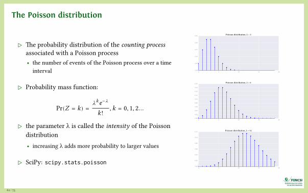
▷ The probability distribution of the counting processassociated with a Poisson process• the number of events of the Poisson process over a time
interval
▷ Probability mass function:
Pr(Z = k) =𝜆ke−u�
k!, k = 0, 1, 2…
▷ the parameter λ is called the intensity of the Poissondistribution• increasing λ adds more probability to larger values
▷ SciPy: scipy.stats.poisson
0 5 10 15 200.00
0.05
0.10
0.15
0.20
0.25 Poisson distribution, λ = 3
0 5 10 15 200.00
0.02
0.04
0.06
0.08
0.10
0.12
0.14
0.16
0.18 Poisson distribution, λ = 6
0 5 10 15 200.00
0.02
0.04
0.06
0.08
0.10
0.12 Poisson distribution, λ = 12
62 / 75

Poisson distribution and Prussian horses
▷ Number of fatalities for the Prussian cavalry resulting frombeing kicked by a horse was recorded over a period of 20 years• for 10 army corps, so total number of observations is 200
Deaths Occurrences0 1091 652 223 34 1> 4 0
▷ It follows a Poisson distribution
▷ Exercise: reproduce the plot on the right which shows a fitbetween a Poisson distribution and the historical data
0 1 2 3 40
20
40
60
80
100
120
Num
ber
of d
eath
s fr
om h
orse
kic
ks (p
er c
orps
per
yea
r)
Prussian army deaths from horse kicksPoisson fitObserved
63 / 75

The Poisson distribution: properties
▷ Expected value of the Poisson distribution is equal to its parameter μ
▷ Variance of the Poisson distribution is equal to its parameter μ
▷ The sum of independent Poisson random variables is also Poisson
▷ Specifically, if Y1 and Y2 are independent with Yi ∼ Poisson(𝜇i) for i = 1, 2then Y1 + Y2 ∼ Poisson(𝜇1 + 𝜇2)
▷ Exercise: test these properties empirically with SciPy
N o t a t i o n :∼ m e a n s “ f o l l o w s
i n d i s t r i b ut i o n ”
64 / 75

Simulating earthquake occurrences (1/2)
▷ Suppose we live in an area where there aretypically 0.05 earthquakes of intensity 5 ormore per year
▷ Assume earthquake arrival is a Poissonprocess• interval between earthquakes follows an
exponential distribution
• events are independent
▷ Simulate the random intervals between thenext earthquakes of intensity 5 or greater
▷ What is the 25th percentile of the intervalbetween 5+ earthquakes?
1 > from scipy.stats import expon
2 > expon.rvs(scale=1/0.03, size=15)
3 array([ 23.23763551, 28.73209684, 29.7729332 , 46.66320369,
4 4.03328973, 84.03262547, 42.22440297, 14.14994806,
5 29.90516283, 87.07194806, 11.25694683, 15.08286603,
6 35.72159516, 44.70480237, 44.67294338])
7 > expon.ppf(0.25, scale=1.0/0.03)
8 9.5894024150593644
65 / 75

Simulating earthquake occurrences (2/2)
▷ Worldwide: 144 earthquakes of magnitude 6 or greaterin 2013 (one every 60.8 hours on average)
▷ rate: λ = 160.8
per hour
▷ What’s the probability that an earthquake ofmagnitude 6 or greater will occur (worldwide) in thenext day?• right: plot of the CDF of the corresponding exponential
distribution
• scipy.stats.expon.cdf(24, scale=60.8) = 0.326
Earthquake locations
0 50 100 150 200 250Elapsed time (hours)
0.0
0.2
0.4
0.6
0.8
1.0
Prob
abili
ty o
f an
eart
hqua
ke
Data source: http://earthquake.usgs.gov/earthquakes/search/
66 / 75

Weibull distribution
0 1 2 3 4 50.0
0.1
0.2
0.3
0.4
0.5
0.6
Weibull distribution PDFk=0.5, λ=1k=1.0, λ=1k=2.0, λ=1k=2.0, λ=2
▷ Very flexible distribution (able to model left-skewed, right-skewed,symmetric data)
▷ Widely used for modeling reliability data
▷ Python: scipy.stats.dweibull(k, 𝜇, 𝜆)
67 / 75
Weibull distribution
0 1 2 3 4 50.0
0.1
0.2
0.3
0.4
0.5
0.6
Weibull distribution PDFk=0.5, λ=1k=1.0, λ=1k=2.0, λ=1k=2.0, λ=2
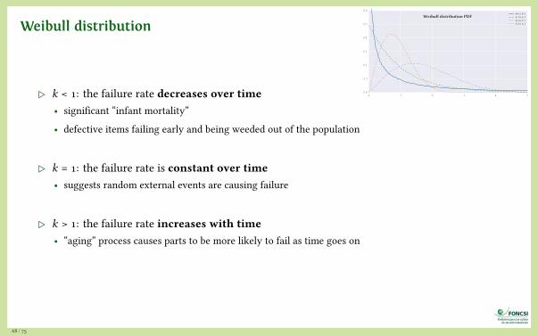
▷ k < 1: the failure rate decreases over time• significant “infant mortality”
• defective items failing early and being weeded out of the population
▷ k = 1: the failure rate is constant over time• suggests random external events are causing failure
▷ k > 1: the failure rate increases with time• “aging” process causes parts to be more likely to fail as time goes on
68 / 75
Student’s t distribution
−4 −2 0 2 40.00
0.05
0.10
0.15
0.20
0.25
0.30
0.35
0.40
0.45 Student’s t distribution PDFt(k=∞)
t(k=2.0)
t(k=1.0)
t(k=0.5)
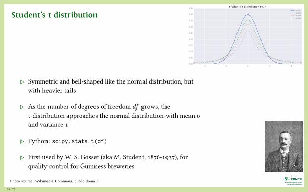
▷ Symmetric and bell-shaped like the normal distribution, butwith heavier tails
▷ As the number of degrees of freedom df grows, thet-distribution approaches the normal distribution with mean 0and variance 1
▷ Python: scipy.stats.t(df)
▷ First used by W. S. Gosset (aka M. Student, 1876-1937), forquality control for Guinness breweries
Photo source: Wikimedia Commons, public domain
69 / 75

Analyzing
data
70 / 75

Curve fitting
▷ Generate 1000 random numbersfrom a normal distributioncentered at 10, stddev of 2
▷ Find median of the sample
▷ Check that 50% quantile is equal tothe median
▷ Find 5% quantile of the sample andcompare with expected analyticvalue
▷ Fit a normal distribution to thesample and check that shapeparameters are appropriate
71 / 75
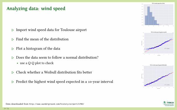
Analyzing data: wind speed
▷ Import wind speed data for Toulouse airport
▷ Find the mean of the distribution
▷ Plot a histogram of the data
▷ Does the data seem to follow a normal distribution?• use a Q-Q plot to check
▷ Check whether a Weibull distribution fits better
▷ Predict the highest wind speed expected in a 10-year interval
0 10 20 30 40 50 600.00
0.01
0.02
0.03
0.04
0.05
0.06
0.07
0.08 TLS wind speed in 2013
−3 −2 −1 0 1 2 3Quantiles
−10
0
10
20
30
40
50
Ord
ered
Val
ues
R2 =0:9645
TLS wind speed qqnorm-plot
0 5 10 15 20 25 30 35Quantiles
0
10
20
30
40
50
Ord
ered
Val
ues
R2 =0:9850
TLS wind speed qqweibull plot
Data downloaded from http://www.wunderground.com/history/airport/LFBO/
72 / 75
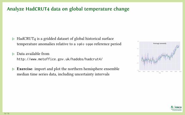
Analyze HadCRUT4 data on global temperature change
▷ HadCRUT4 is a gridded dataset of global historical surfacetemperature anomalies relative to a 1961-1990 reference period
▷ Data available fromhttp://www.metoffice.gov.uk/hadobs/hadcrut4/
▷ Exercise: import and plot the northern hemisphere ensemblemedian time series data, including uncertainty intervals
1840 1860 1880 1900 1920 1940 1960 1980 2000 2020Year
−1.0
−0.5
0.0
0.5
1.0
Average anomaly
73 / 75

Image credits
▷ Dice on slide 39, https://flic.kr/p/9SJ5g, CC BY-NC-ND licence
▷ Microscope on slide 70 adapted from https://flic.kr/p/aeh1J5, CC BYlicence
74 / 75
For more information
▷ SciPy lecture notes: scipy-lectures.github.io/
▷ Book Statistics done wrong, available online at statisticsdonewrong.com
▷ A gallery of interesting IPython notebooks:github.com/ipython/ipython/wiki/A-gallery-of-interesting-IPython-Notebooks
This presentation is distributed under the terms ofthe Creative Commons Attribution – Share Alikelicence.
SKRENGINEERING
For more free course materials on risk engineering, visithttp://risk-engineering.org/
75 / 75