slides CIRM copulas, extremes and actuarial science

Arthur CHARPENTIER - Probit transformation for nonparametric kernel estimation of the copula

Probit transformation for nonparametric kernel estimation of the copula

A. Charpentier (Université de Rennes 1 & UQAM),

joint work with G. Geenens (UNSW) & D. Paindaveine (ULB)

CIRM Workshop “Extremes - Copulas - Actuarial science”, February 2016

http://arxiv.org/abs/1404.4414, to appear in Bernoulli

url: http://freakonometrics.hypotheses.orgemail : [email protected]

: @freakonometrics

1


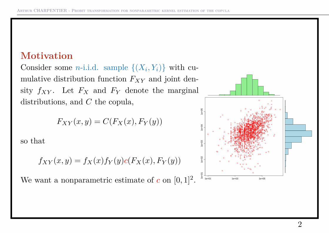
MotivationConsider some n-i.i.d. sample {(Xi, Yi)} with cu-mulative distribution function FXY and joint den-sity fXY . Let FX and FY denote the marginaldistributions, and C the copula,

FXY (x, y) = C(FX(x), FY (y))

so that

fXY (x, y) = fX(x)fY (y)c(FX(x), FY (y))

We want a nonparametric estimate of c on [0, 1]2. 1e+01 1e+03 1e+051e+

011e

+02

1e+

031e

+04

1e+

05

2


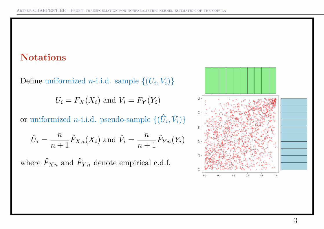
Notations

Define uniformized n-i.i.d. sample {(Ui, Vi)}

Ui = FX(Xi) and Vi = FY (Yi)

or uniformized n-i.i.d. pseudo-sample {(Ui, Vi)}

Ui = n

n+ 1 FXn(Xi) and Vi = n

n+ 1 FY n(Yi)

where FXn and FY n denote empirical c.d.f.0.0 0.2 0.4 0.6 0.8 1.0

0.0

0.2

0.4

0.6

0.8

1.0

3


Standard Kernel EstimateThe standard kernel estimator for c, say c∗, at (u, v) ∈ I would be (see Wand &Jones (1995))

c∗(u, v) = 1n|HUV |1/2

n∑i=1

K(

H−1/2UV

(u− Uiv − Vi

)), (1)

where K : R2 → R is a kernel function and HUV is a bandwidth matrix.

4


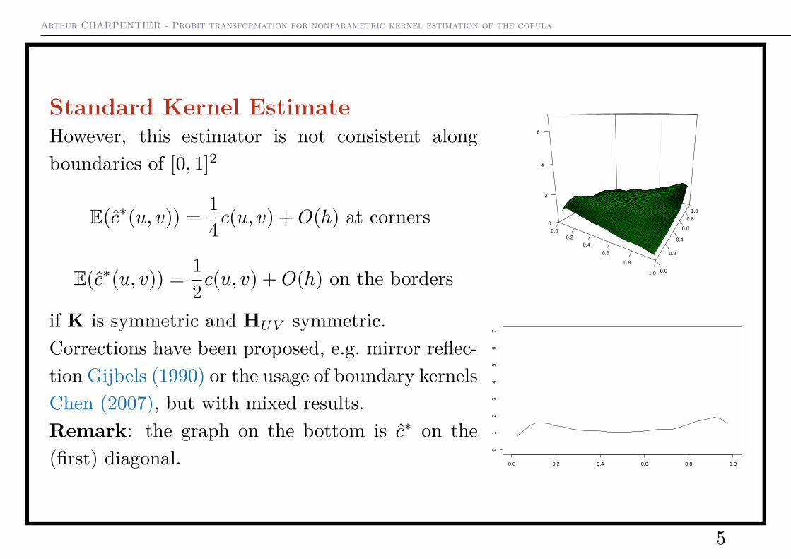
Standard Kernel EstimateHowever, this estimator is not consistent alongboundaries of [0, 1]2

E(c∗(u, v)) = 14c(u, v) +O(h) at corners

E(c∗(u, v)) = 12c(u, v) +O(h) on the borders

if K is symmetric and HUV symmetric.Corrections have been proposed, e.g. mirror reflec-tion Gijbels (1990) or the usage of boundary kernelsChen (2007), but with mixed results.Remark: the graph on the bottom is c∗ on the(first) diagonal.

0.00.2

0.4

0.6

0.8

1.0 0.0

0.2

0.4

0.6

0.8

1.0

0

2

4

6

0.0 0.2 0.4 0.6 0.8 1.0

01

23

45

67

5


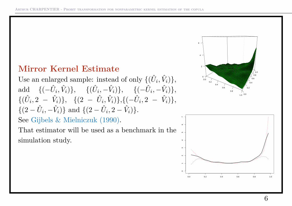
Mirror Kernel EstimateUse an enlarged sample: instead of only {(Ui, Vi)},add {(−Ui, Vi)}, {(Ui,−Vi)}, {(−Ui,−Vi)},{(Ui, 2 − Vi)}, {(2 − Ui, Vi)},{(−Ui, 2 − Vi)},{(2− Ui,−Vi)} and {(2− Ui, 2− Vi)}.See Gijbels & Mielniczuk (1990).That estimator will be used as a benchmark in thesimulation study.

0.00.2

0.4

0.6

0.8

1.0 0.0

0.2

0.4

0.6

0.8

1.0

0

2

4

6

0.0 0.2 0.4 0.6 0.8 1.0

01

23

45

67

6


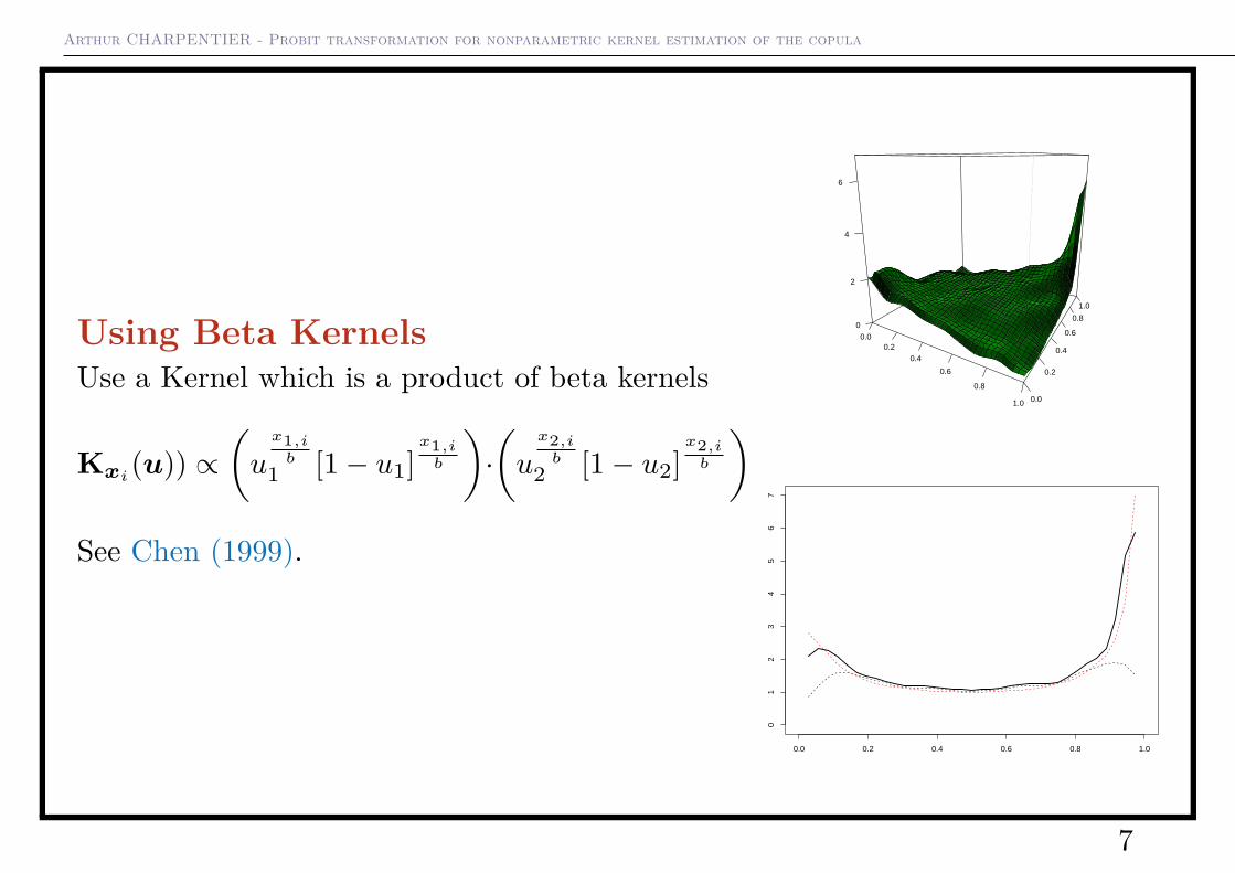
Using Beta KernelsUse a Kernel which is a product of beta kernels

Kxi(u)) ∝

(u

x1,ib

1 [1− u1]x1,i

b

)·(u

x2,ib

2 [1− u2]x2,i

b

)See Chen (1999).

0.00.2

0.4

0.6

0.8

1.0 0.0

0.2

0.4

0.6

0.8

1.0

0

2

4

6

0.0 0.2 0.4 0.6 0.8 1.0

01

23

45

67

7


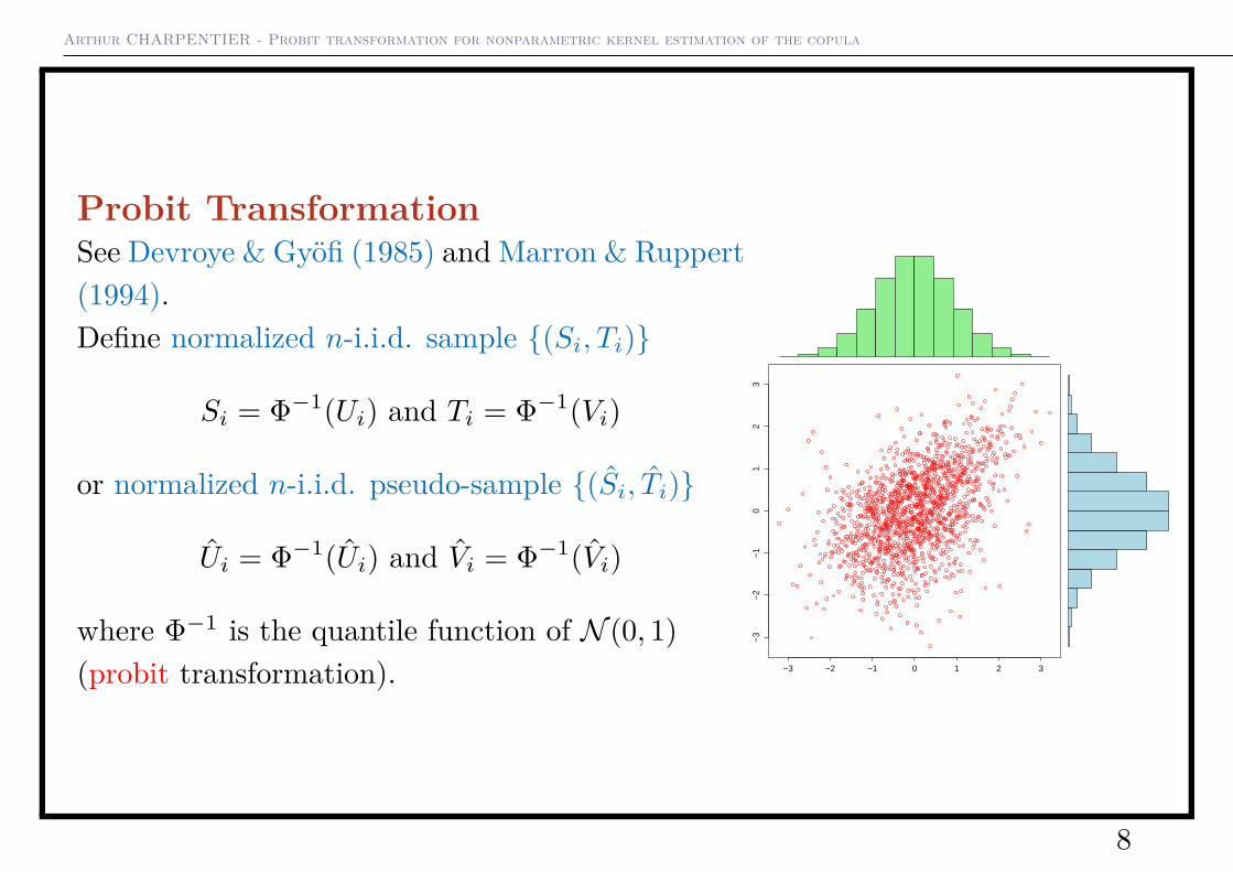
Probit TransformationSee Devroye & Gyöfi (1985) and Marron & Ruppert(1994).Define normalized n-i.i.d. sample {(Si, Ti)}

Si = Φ−1(Ui) and Ti = Φ−1(Vi)

or normalized n-i.i.d. pseudo-sample {(Si, Ti)}

Ui = Φ−1(Ui) and Vi = Φ−1(Vi)

where Φ−1 is the quantile function of N (0, 1)(probit transformation). −3 −2 −1 0 1 2 3

−3

−2

−1

01

23

8


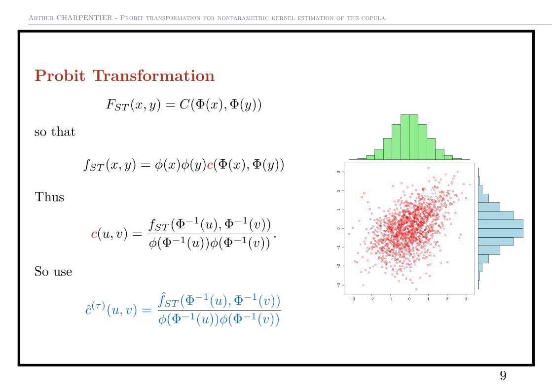
Probit TransformationFST (x, y) = C(Φ(x),Φ(y))

so that

fST (x, y) = φ(x)φ(y)c(Φ(x),Φ(y))

Thus

c(u, v) = fST (Φ−1(u),Φ−1(v))φ(Φ−1(u))φ(Φ−1(v)) .

So use

c(τ)(u, v) = fST (Φ−1(u),Φ−1(v))φ(Φ−1(u))φ(Φ−1(v))

−3 −2 −1 0 1 2 3

−3

−2

−1

01

23

9


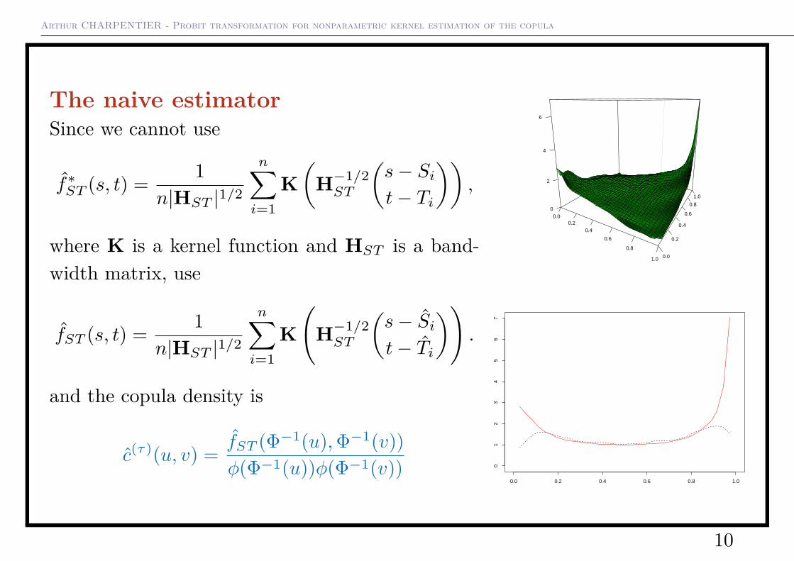
The naive estimatorSince we cannot use

f∗ST (s, t) = 1n|HST |1/2

n∑i=1

K(

H−1/2ST

(s− Sit− Ti

)),

where K is a kernel function and HST is a band-width matrix, use

fST (s, t) = 1n|HST |1/2

n∑i=1

K(

H−1/2ST

(s− Sit− Ti

)).

and the copula density is

c(τ)(u, v) = fST (Φ−1(u),Φ−1(v))φ(Φ−1(u))φ(Φ−1(v))

0.00.2

0.4

0.6

0.8

1.0 0.0

0.2

0.4

0.6

0.8

1.0

0

2

4

6

0.0 0.2 0.4 0.6 0.8 1.0

01

23

45

67

10


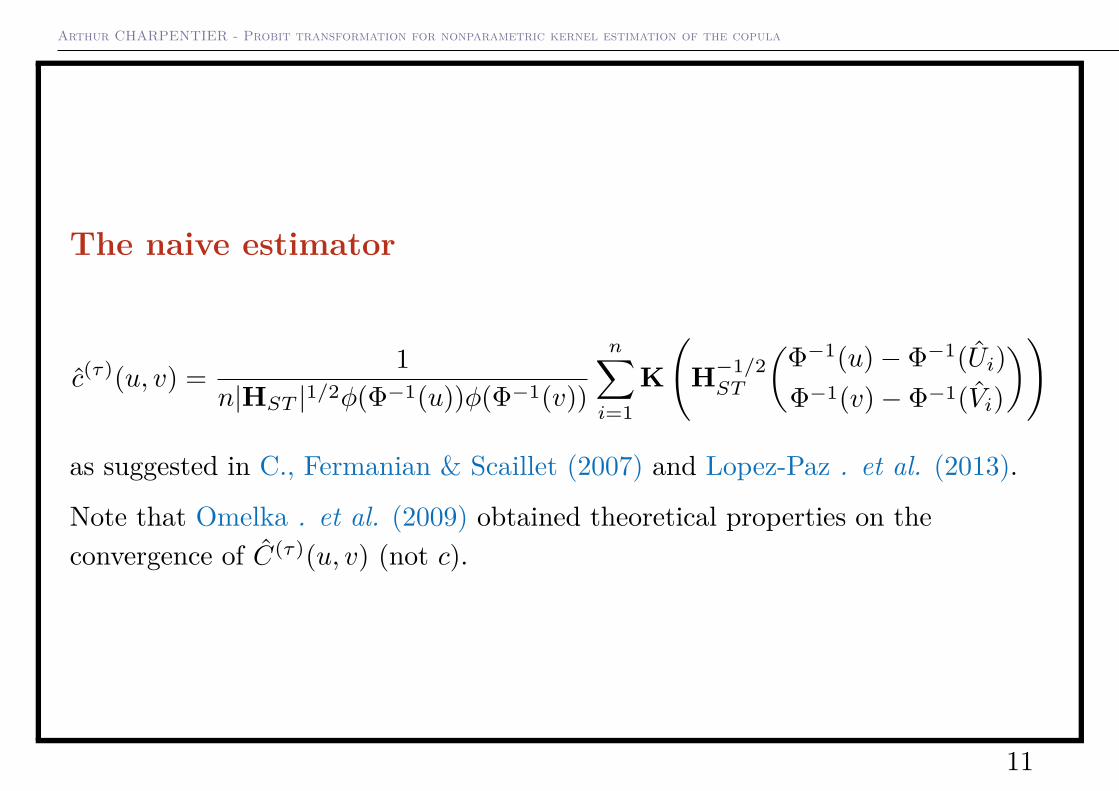
The naive estimator

c(τ)(u, v) = 1n|HST |1/2φ(Φ−1(u))φ(Φ−1(v))

n∑i=1

K(

H−1/2ST

(Φ−1(u)− Φ−1(Ui)Φ−1(v)− Φ−1(Vi)

))

as suggested in C., Fermanian & Scaillet (2007) and Lopez-Paz . et al. (2013).

Note that Omelka . et al. (2009) obtained theoretical properties on theconvergence of C(τ)(u, v) (not c).

11


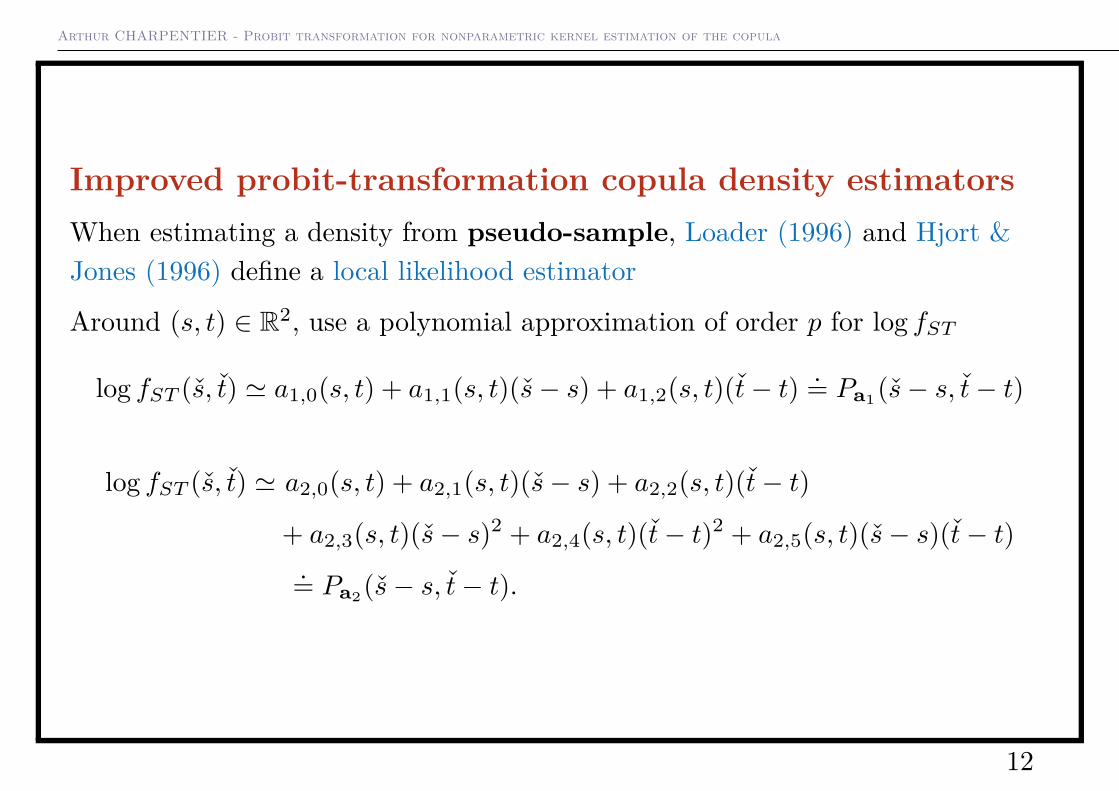
Improved probit-transformation copula density estimatorsWhen estimating a density from pseudo-sample, Loader (1996) and Hjort &Jones (1996) define a local likelihood estimator

Around (s, t) ∈ R2, use a polynomial approximation of order p for log fST

log fST (s, t) ' a1,0(s, t) + a1,1(s, t)(s− s) + a1,2(s, t)(t− t) .= Pa1(s− s, t− t)

log fST (s, t) ' a2,0(s, t) + a2,1(s, t)(s− s) + a2,2(s, t)(t− t)

+ a2,3(s, t)(s− s)2 + a2,4(s, t)(t− t)2 + a2,5(s, t)(s− s)(t− t).= Pa2(s− s, t− t).

12


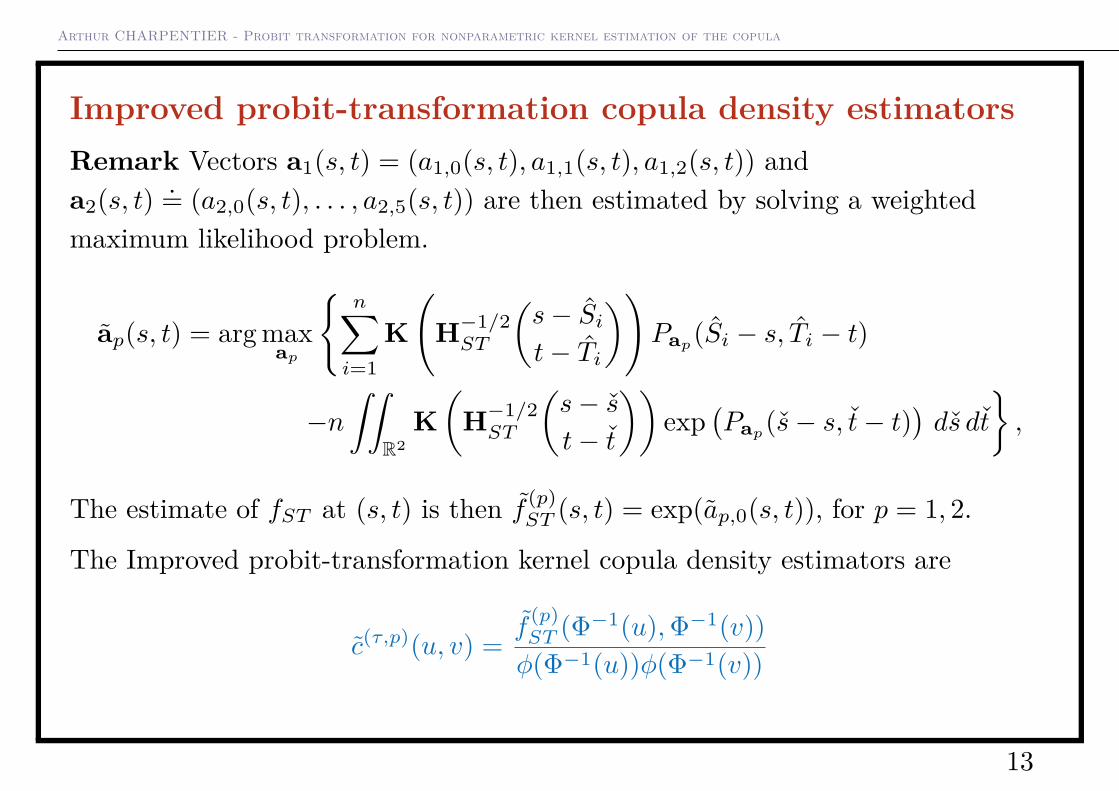
Improved probit-transformation copula density estimatorsRemark Vectors a1(s, t) = (a1,0(s, t), a1,1(s, t), a1,2(s, t)) anda2(s, t) .= (a2,0(s, t), . . . , a2,5(s, t)) are then estimated by solving a weightedmaximum likelihood problem.

ap(s, t) = arg maxap

{n∑i=1

K(

H−1/2ST

(s− Sit− Ti

))Pap

(Si − s, Ti − t)

−n∫∫

R2K(

H−1/2ST

(s− st− t

))exp

(Pap(s− s, t− t)

)ds dt

},

The estimate of fST at (s, t) is then f (p)ST (s, t) = exp(ap,0(s, t)), for p = 1, 2.

The Improved probit-transformation kernel copula density estimators are

c(τ,p)(u, v) = f(p)ST (Φ−1(u),Φ−1(v))φ(Φ−1(u))φ(Φ−1(v))

13


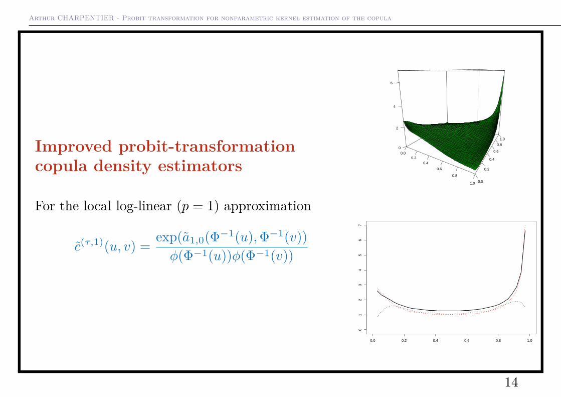
Improved probit-transformationcopula density estimators

For the local log-linear (p = 1) approximation

c(τ,1)(u, v) = exp(a1,0(Φ−1(u),Φ−1(v))φ(Φ−1(u))φ(Φ−1(v))

0.00.2

0.4

0.6

0.8

1.0 0.0

0.2

0.4

0.6

0.8

1.0

0

2

4

6

0.0 0.2 0.4 0.6 0.8 1.0

01

23

45

67

14


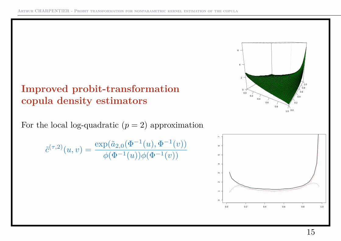
Improved probit-transformationcopula density estimators

For the local log-quadratic (p = 2) approximation

c(τ,2)(u, v) = exp(a2,0(Φ−1(u),Φ−1(v))φ(Φ−1(u))φ(Φ−1(v))

0.00.2

0.4

0.6

0.8

1.0 0.0

0.2

0.4

0.6

0.8

1.0

0

2

4

6

0.0 0.2 0.4 0.6 0.8 1.0

01

23

45

67

15


Asymptotic propertiesA1. The sample {(Xi, Yi)} is a n- i.i.d. sample from the joint distribution FXY ,an absolutely continuous distribution with marginals FX and FY strictlyincreasing on their support;

(uniqueness of the copula)

16


Asymptotic propertiesA2. The copula C of FXY is such that (∂C/∂u)(u, v) and (∂2C/∂u2)(u, v) existand are continuous on {(u, v) : u ∈ (0, 1), v ∈ [0, 1]}, and (∂C/∂v)(u, v) and(∂2C/∂v2)(u, v) exist and are continuous on {(u, v) : u ∈ [0, 1], v ∈ (0, 1)}. Inaddition, there are constants K1 and K2 such that

∣∣∣∣∂2C

∂u2 (u, v)∣∣∣∣ ≤ K1

u(1− u) for (u, v) ∈ (0, 1)× [0, 1];∣∣∣∣∂2C

∂v2 (u, v)∣∣∣∣ ≤ K2

v(1− v) for (u, v) ∈ [0, 1]× (0, 1);

A3. The density c of C exists, is positive and admits continuous second-orderpartial derivatives on the interior of the unit square I. In addition, there is aconstant K00 such that

c(u, v) ≤ K00 min(

1u(1− u) ,

1v(1− v)

)∀(u, v) ∈ (0, 1)2.

see Segers (2012).

17


Asymptotic propertiesAssume that K(z1, z2) = φ(z1)φ(z2) and HST = h2I with h ∼ n−a for somea ∈ (0, 1/4). Under Assumptions A1-A3, the ‘naive’ probit transformation kernelcopula density estimator at any (u, v) ∈ (0, 1)2 is such that√nh2

(c(τ)(u, v)− c(u, v)− h2 b(u, v)

φ(Φ−1(u))φ(Φ−1(v))

)L−→ N

(0, σ2(u, v)

),

where b(u, v) = 12

{∂2c

∂u2 (u, v)φ2(Φ−1(u)) + ∂2c

∂v2 (u, v)φ2(Φ−1(v))

− 3(∂c

∂u(u, v)Φ−1(u)φ(Φ−1(u)) + ∂c

∂v(u, v)Φ−1(v)φ(Φ−1(v))

)+ c(u, v)

({Φ−1(u)}2 + {Φ−1(v)}2 − 2

)}(2)

and σ2(u, v) = c(u, v)4πφ(Φ−1(u))φ(Φ−1(v)) .

18


The Amended versionThe last unbounded term in b be easily adjusted.

c(τam)(u, v) = fST (Φ−1(u),Φ−1(v))φ(Φ−1(u))φ(Φ−1(v)) ×

11 + 1

2h2 ({Φ−1(u)}2 + {Φ−1(v)}2 − 2)

.

The asymptotic bias becomes proportional to

b(am)(u, v) = 12

{∂2c

∂u2 (u, v)φ2(Φ−1(u)) + ∂2c

∂v2 (u, v)φ2(Φ−1(v))

−3(∂c

∂u(u, v)Φ−1(u)φ(Φ−1(u)) + ∂c

∂v(u, v)Φ−1(v)φ(Φ−1(v))

)}.

19


A local log-linear probit-transformation kernel estimator

c∗(τ,1)(u, v) = f∗(1)ST (Φ−1(u),Φ−1(v))/

(φ(Φ−1(u))φ(Φ−1(v))

)Then√nh2

(c∗(τ,1)(u, v)− c(u, v)− h2 b(1)(u, v)

φ(Φ−1(u))φ(Φ−1(v))

)L−→ N

(0, σ(1) 2

(u, v)),

where b(1)(u, v) = 12

{∂2c

∂u2 (u, v)φ2(Φ−1(u)) + ∂2c

∂v2 (u, v)φ2(Φ−1(v))

− 1c(u, v)

({∂c

∂u(u, v)

}2φ2(Φ−1(u)) +

{∂c

∂v(u, v)

}2φ2(Φ−1(v))

)

−(∂c

∂u(u, v)Φ−1(u)φ(Φ−1(u)) + ∂c

∂v(u, v)Φ−1(v)φ(Φ−1(v))

)− 2c(u, v)

}

20


Using a higher order polynomial approximationLocally fitting a polynomial of a higher degree is known to reduce the asymptoticbias of the estimator, here from order O(h2) to order O(h4), see Loader (1996) orHjort (1996), under sufficient smoothness conditions.

If fST admits continuous fourth-order partial derivatives and is positive at (s, t),then

√nh2

(f∗(2)ST (s, t)− fST (s, t)− h4b

(2)ST (s, t)

)L−→ N

(0, σ(2)

ST

2(s, t)

),

where σ(2)ST

2(s, t) = 5

2fST (s, t)

4π and

b(2)ST (s, t) = −1

8fST (s, t)

×{(

∂4g

∂s4 + ∂4g

∂t4

)+ 4

(∂3g

∂s3∂g

∂s+ ∂3g

∂t3∂g

∂t+ ∂3g

∂s2∂t

∂g

∂t+ ∂3g

∂s∂t2∂g

∂s

)+ 2 ∂4g

∂s2∂t2

}(s, t),

with g(s, t) = log fST (s, t).

21


Using a higher order polynomial approximationA4. The copula density c(u, v) = (∂2C/∂u∂v)(u, v) admits continuousfourth-order partial derivatives on the interior of the unit square [0, 1]2.

Then

√nh2

(c∗(τ,2)(u, v)− c(u, v)− h4 b(2)(u, v)

φ(Φ−1(u))φ(Φ−1(v))

)L−→ N

(0, σ(2) 2

(u, v))

where σ(2) 2(u, v) = 5

2c(u, v)

4πφ(Φ−1(u))φ(Φ−1(v))

22


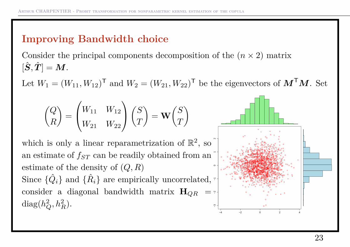
Improving Bandwidth choiceConsider the principal components decomposition of the (n× 2) matrix[S, T ] = M .

Let W1 = (W11,W12)T and W2 = (W21,W22)T be the eigenvectors of MTM . Set

(Q

R

)=

W11 W12

W21 W22

(ST

)= W

(S

T

)which is only a linear reparametrization of R2, soan estimate of fST can be readily obtained from anestimate of the density of (Q,R)Since {Qi} and {Ri} are empirically uncorrelated,consider a diagonal bandwidth matrix HQR =diag(h2

Q, h2R).

−4 −2 0 2 4−

3−

2−

10

12

23


Improving Bandwidth choiceUse univariate procedures to select hQ and hR independently

Denote f (p)Q and f (p)

R (p = 1, 2), the local log-polynomial estimators for thedensities

hQ can be selected via cross-validation (see Section 5.3.3 in Loader (1999))

hQ = arg minh>0

{∫ ∞−∞

{f

(p)Q (q)

}2dq − 2

n

n∑i=1

f(p)Q(−i)(Qi)

},

where f (p)Q(−i) is the ‘leave-one-out’ version of f (p)

Q .

24


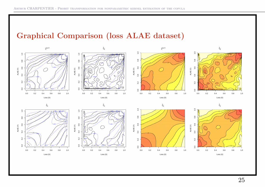
Graphical Comparison (loss ALAE dataset)c~(τ2)

Loss (X)

ALA

E (

Y)

0.25

0.25

0.5

0.5

0.75

0.75

1

1

1.25

1.25

1.5

1.5

2

2

4

0.0 0.2 0.4 0.6 0.8 1.0

0.0

0.2

0.4

0.6

0.8

1.0

0.25

0.2

5

0.5

0.5

0.75

0.75

1

1

1

1.25

1.25

1.5

1.5

2

2

4

cβ

Loss (X)

ALA

E (

Y)

0.25

0.25

0.5

0.5

0.75

0.75

1

1

1.25

1.25

1.5

1.5

2

2

4

0.0 0.2 0.4 0.6 0.8 1.0

0.0

0.2

0.4

0.6

0.8

1.0

0.25 0.25

0.25 0.25

0.5

0.5

0.75

0.75

0.75

1

1

1

1

1

1.25

1.25

1.25

1.25

1.25

1.5

1.5

2 2

2

4

cb

Loss (X)

ALA

E (

Y)

0.25

0.25

0.5

0.5

0.75

0.75

1

1

1.25

1.25

1.5

1.5

2

2

4

0.0 0.2 0.4 0.6 0.8 1.0

0.0

0.2

0.4

0.6

0.8

1.0

0.25

0.2

5

0.5

0.5

0.75

0.75 1 1

1.25

1.25

1.5

1.5

2

2

cp

Loss (X)

ALA

E (

Y)

0.25

0.25

0.5

0.5

0.75

0.75

1

1

1.25

1.25

1.5

1.5

2

2

4

0.0 0.2 0.4 0.6 0.8 1.0

0.0

0.2

0.4

0.6

0.8

1.0

0.25

0.25

0.25

0.2

5

0.5

0.5

0.75

0.75

1

1

1

1.25

1.25

1.25

1.25

1.5

1.5

1.5

2

2

4

0.0 0.2 0.4 0.6 0.8 1.0

0.0

0.2

0.4

0.6

0.8

1.0

c~(τ2)

Loss (X)

ALA

E (

Y)

0.25

0.2

5

0.5

0.5

0.75

0.75

1

1

1

1.25

1.25

1.5

1.5

2

2

4

0.0 0.2 0.4 0.6 0.8 1.0

0.0

0.2

0.4

0.6

0.8

1.0

cβ

Loss (X)

ALA

E (

Y)

0.25 0.25

0.25 0.25

0.5

0.5

0.75

0.75

0.75

1

1

1

1

1

1.25

1.25

1.25

1.25

1.25

1.5

1.5

1.5

2

2

2

4

0.0 0.2 0.4 0.6 0.8 1.0

0.0

0.2

0.4

0.6

0.8

1.0

cb

Loss (X)

ALA

E (

Y)

0.25

0.2

5

0.5

0.5

0.75

0.75 1

1

1.25

1.25

1.5

1.5

2

2

0.0 0.2 0.4 0.6 0.8 1.0

0.0

0.2

0.4

0.6

0.8

1.0

cp

Loss (X)

ALA

E (

Y)

0.25

0.25

0.25

0.2

5

0.5

0.5

0.75

0.75

1

1

1

1.25

1.25

1.25

1.25

1.5

1.5

1.5

2

2

4

25


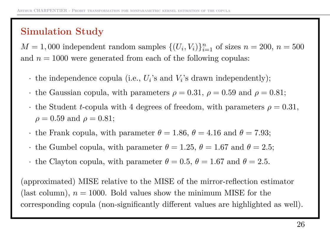
Simulation StudyM = 1, 000 independent random samples {(Ui, Vi)}ni=1 of sizes n = 200, n = 500and n = 1000 were generated from each of the following copulas:

· the independence copula (i.e., Ui’s and Vi’s drawn independently);

· the Gaussian copula, with parameters ρ = 0.31, ρ = 0.59 and ρ = 0.81;

· the Student t-copula with 4 degrees of freedom, with parameters ρ = 0.31,ρ = 0.59 and ρ = 0.81;

· the Frank copula, with parameter θ = 1.86, θ = 4.16 and θ = 7.93;

· the Gumbel copula, with parameter θ = 1.25, θ = 1.67 and θ = 2.5;

· the Clayton copula, with parameter θ = 0.5, θ = 1.67 and θ = 2.5.

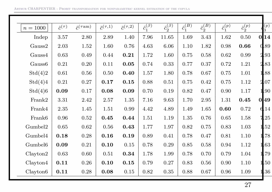
(approximated) MISE relative to the MISE of the mirror-reflection estimator(last column), n = 1000. Bold values show the minimum MISE for thecorresponding copula (non-significantly different values are highlighted as well).

26


n = 1000 c(τ) c(τam) c(τ,1) c(τ,2) c(β)1 c

(β)2 c

(B)1 c

(B)2 c

(p)1 c

(p)2 c

(p)3 c(m)

Indep 3.57 2.80 2.89 1.40 7.96 11.65 1.69 3.43 1.62 0.50 0.14 0.01Gauss2 2.03 1.52 1.60 0.76 4.63 6.06 1.10 1.82 0.98 0.66 0.89 0.01Gauss4 0.63 0.49 0.44 0.21 1.72 1.60 0.75 0.58 0.62 0.99 2.93 0.05Gauss6 0.21 0.20 0.11 0.05 0.74 0.33 0.77 0.37 0.72 1.21 2.83 0.26Std(4)2 0.61 0.56 0.50 0.40 1.57 1.80 0.78 0.67 0.75 1.01 1.88 0.04Std(4)4 0.21 0.27 0.17 0.15 0.88 0.51 0.75 0.42 0.75 1.12 2.07 0.16Std(4)6 0.09 0.17 0.08 0.09 0.70 0.19 0.82 0.47 0.90 1.17 1.90 0.67Frank2 3.31 2.42 2.57 1.35 7.16 9.63 1.70 2.95 1.31 0.45 0.49 0.01Frank4 2.35 1.45 1.51 0.99 4.42 4.89 1.49 1.65 0.60 0.72 6.14 0.01Frank6 0.96 0.52 0.45 0.44 1.51 1.19 1.35 0.76 0.65 1.58 7.25 0.07

Gumbel2 0.65 0.62 0.56 0.43 1.77 1.97 0.82 0.75 0.83 1.03 1.52 0.04Gumbel4 0.18 0.28 0.16 0.19 0.89 0.41 0.78 0.47 0.81 1.10 1.78 0.21Gumbel6 0.09 0.21 0.10 0.15 0.78 0.29 0.85 0.58 0.94 1.12 1.63 0.93Clayton2 0.63 0.60 0.51 0.34 1.78 1.99 0.78 0.70 0.79 1.04 1.79 0.04Clayton4 0.11 0.26 0.10 0.15 0.79 0.27 0.83 0.56 0.90 1.10 1.50 0.65Clayton6 0.11 0.28 0.08 0.15 0.82 0.35 0.88 0.67 0.96 1.09 1.36 1.61

27

Data & Analytics

slides CIRM copulas, extremes and actuarial science