Regression

© aSup-2007

INTRODUCTION TO REGRESSION

1

CORRELATION• … is a statistical technique that used to

measure and describe a relationship between two variables

• Usually the two variables are simply observed as they exist naturally in environment, there is no attempt to control or manipulate the variables

© aSup-2007


2


© aSup-2007


3

PREVIEW• We noted that one common application

of correlation is for purposes of prediction

• Whenever there is a consistent relationship between two variables, it is possible to use the value of one variable to predict the value of another

• The general statistical process of finding and using a prediction equation is known as REGRESSION

© aSup-2007


4

INTRODUCTION• Our goal in this section is to develop a

procedure that identifies and defines the straight line that provide the best fit for any specific set of data

• You should realize that this straight line does not have to be drawn on a graph; it can be presented in a simple equation

• Thus, our goal is to find the equation for the line that best describe s the relation for a set of X and Y data

© aSup-2007


5

LINEAR EQUATION• In general, a linear relationship between

two variables X and Y can be expressed by the equation

Y = bX + awhere a and b are fixed constant

• In general linear equation, the value of b is called the slope

• The slope determines how much the Y variable will change when X is increase by one point

© aSup-2007


6

EXAMPLE• A local tennis club charges a fee of Rp

20.000 per hour plus an annual membership of fee of Rp 100.000

• With this information the total cost of playing tennis can be computed using a linear equation that describe the relationship between the total cost (Y) and the number of hours (X)

Y = 20.000(hour) + 100.00

© aSup-2007


7

H

Total Cost Y

1 2 3 4 5 6 7 8

240

220

200

180

160

140

120

100

0

© aSup-2007


8

THE LEAST-SQUARED ERROR• To determine how well a line fits the

data points, the first step is to define mathematically distance between the line and each data point

• For every X value in the data, the linear equation will determine a Y value on the line

© aSup-2007


9

IQ

IPK

90 95 100 105 110 115 120 125 130 135

4.00

3.50

3.00

2.50

2.00

1.50

1.00

0.50

0

Data Point

distance

© aSup-2007


10

THE LEAST-SQUARED ERROR• To determine how well a line fits the data

points, the fist step is to define mathematically distance between the line and each data point

• For every X value in the data, the linear equation will determine a Y value on the line

• This value is the predicted Y an is called Ŷ (‘y hat’)

• The distance between this predicted value and the actual Y value in the data is determined by

distance = Y - Ŷ

© aSup-2007


11

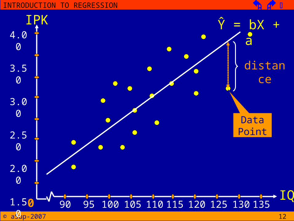
THE LEAST-SQUARED ERROR• Notice that we are simply are measuring the

vertical distance between the actual data point (Y) and the predicted point on the line

• The distance measure the error between the line and the actual data

• Because some of these distance will be positive and some will be negative, the next sep is to square each distance in order to obtain a uniformity positive measure of error

total squared error = Σ(Y - Ŷ)2

© aSup-2007


12

IQ

IPK

90 95 100 105 110 115 120 125 130 135

4.00

3.50

3.00

2.50

2.00

1.50

1.00

0.50

0

Data Point

distance

Ŷ = bX + a

© aSup-2007


13

The EQUATION

Ŷ = bX + a

b =SP

SSX

a = MY - bMX

© aSup-2007


14

EXAMPLEX Y X – MX Y – MY (X-MX)(Y-MY) (X-

MX)2

7

4

6

3

5

11

3

5

4

7

2

-1

1

-2

0

5

-3

-1

-2

1

10

3

-1

4

0

4

1

1

4

0

b =SP

SSX

= 1,6 a = MY – bMX = -2Ŷ = 1,6X - 2

© aSup-2007


15

X

Y

1 2 3 4 5 6 7

11109876543210

Ŷ = 1,6X - 2

© aSup-2007


16

TWO CAUTIONS SHOULD BE CONSIDERED

• The predicted value is not perfect (unless r = +1.00 or -1.00)it should be clear that the data points do

not fit perfectly on the line

• The regression equation should not be used to make prediction for X values that fall outside the range values covered by the original data

© aSup-2007


17

MULTIPLE REGRESSION WITH SOME PREDICTOR VARIABLES

Ŷ = b1X1 + b2X2 + b3X3 + … + a

© aSup-2007


Dasar Pemikiran• Dalam pengukuran psikologis, kita hanya dapat

memperkirakan besarnya atribut yang hendak diukur.

• Dua kali pengukuran dalam atribut yang sama pada subyek A bisa memberikan hasil yang berbeda berapa skor A yang sesungguhnya dalam atribut ini?

• Dengan demikian, sebuah hasil pengukuran (skor A) tidak dapat memberikan gambaran yang sesungguhnya /akurat dari atribut tertentu pada A (Spearman).

• Dengan kata lain, setiap pengukuran akan selalu mengandung “error” yang disebut sebagai error of measurement.

18

© aSup-2007


19

STANDARD ERROR OF MEASUREMENT

• Koefisien reliabilitas menunjukkan konsistensi antara beberapa hasil pengukuran pada subjek yang sama.

• Bahwa setiap pengukuran berharap dapat mengetahui true score seseorang.

• Bagaimana memperkirakan true score seseorang?

© aSup-2007


20


• Bila subyek dites berulang kali (n kali) dengan tes yang sama, maka distribusi skor tes akan menyebar menurut kurva normal.

• Mean dari distribusi skor tes adalah estimated true score.

• Standard deviation dari penyebaran skor tes disebut standard error of measurement.

© aSup-2007


21


SE= standard error of measurement (SEM)

SX= standar deviasi obtained score

rXX= koefisien reliabilitas

Besarnya SEM menunjukkan indeks rata-rata jumlah error dalam skor tes tersebut.

xxXE rSS 1

© aSup-2007


22


• Diasumsikan bahwa random error of measurement berdistribusi secara normal.

• Dengan tingkat kepercayaan tertentu, rentang true score seseorang dapat diperkirakan dari nilai SEM.

• Tingkat kepercayaan 68% (LOC 68%): True Score = X ± 1 SEM• Tingkat kepercayaan 95% (LOC 95%): True Score = X ± 1,96 SEM

© aSup-2007


23

MEMAKNAI SKOR TES• Informasi mengenai koefisien reliabilitas

penting jika kita ingin mengetahui kualitas tes, tapi jika ingin memaknai skor individu maka perlu mengetahui SEM.

• Info bahwa koefisien reliabilitas tes PQN = 0,64 tidak dapat membantu menafsirkan hasil tes yang diperoleh Nina (skor 45) dan Nani (skornya 54).

© aSup-2007


24

MEMAKNAI SKOR TES• Di lain pihak info bahwa SEM = 6 (didapat

bila SX = 10) maka kita dapat menyimpulkan hal-hal berikut:

1. Ada 68,26% kemungkinan skor Nina (X = 45) berkisar antara 39 – 51 dan ada 99% kemungkinan kisarannya 45 ± 2,58 x 6.

2. Ada 68,26% kemungkinan skor Nani (X = 54) ada diantara 48 – 60 dan ada 99% kemungkinan kisarannya 54 ± 2,58 x 6

Jadi masih ada kemungkinan bahwa tidak ada beda antara Nani dan Nina.

© aSup-2007


25

MEMAKNAI SKOR TES (dengan 1 SEM)

45Nina

54Nani

5139 6048X

Data & Analytics

Regression