Recursive Bayesian estimation of ECHO state recurrent neural networks - Branimir Todorovic

Recursive Bayesian Estimation of ECHO state Recurrent Neural Networks

Branimir Todorović

Faculty of Natural Sciences and Mathematics, University of Nišand

Institute NIRI Ltd.

1

12 October 2016Data Science 2016

12 October 2016Data Science 2016 2

OUTLINE

1. Recursive Bayesian Estimation1.1 State Space Model of a Dynamic Sistem1.2 Optimal Solution

2. Recurrent Neural Networks2.1 Recurrent Neural Networks of Old2.2 Reservoir Computing Neural Networks – ECHO state network2.3 Reservoir Computing Neural Networks – NARX RNN

3. State Space Models of Recurrent Neural Networks3.1 SSM of Fully Connected RNN3.2 SSM of Elman RNN3.3 SSM of NARX RNN3.4 SSM of ECHO RNN

4. Computationaly Tractable Approximate Recursive Bayesian Estimation4.1 Linear Minimum Mean Square Error Estimation4.2 Propagating Random Variable through nonlinear mapping

5. Examples

3

1. Recursive Bayesian Estimation1.1 State Space Model of a Dynamic System

Time evolution of the state – dynamic equation:

),,( 1 kkkkk duxfx

Observation of the state is obtained by observation equation:

),( kkkk vxhy

stateprocess noise

known input

observation

state

observation noise

State Space Model of a Dynamic System

Input variables : control and noise .

Output variables: variables of interest that can be either measured or calculated.

State variables: minimum set of variables, whose values completely summarize

the system’s status and which are not directly observable (measurable).

),,( kkk vdu ku ),( kk vd


4


What is known?

a) Sequences of inputs and observations: ),( :0:0 kk yu

b) Exact analytical forms of the dynamics and the observation

process: kk hf ,

c) Noise models )(),( kk vpdp

What should be estimated?

Estimate recursively probability density function (pdf) of the state :

given the input and

the observation sequence .

kx

?)( :0 kk yxp

,...}1,0,{:0 kuu kk

,...}1,0,{:0 kyy kk

1. Recursive Bayesian Estimation1.2 Optimal Solution

5


)()(

)()( 1:0

1:0:0

kkkk

kkkk yxp

yyp

xypyxp

Likelihood

Evidence

Prior

Posterior

Bayes theorem

)( 1:01 kk yxp

11:0111:0 )()()( kkkkkkk dxyxpxxpyxp

kkkkkkk dxyxpxypyyp )()()( 1:01:0

Propagate through the dynamic equation to obtain a prediction of the

state:

Propagate through the observation equation to obtain a prediction of

the observation:

)( 1:0 kk yxp

kkkkkkkk ddpduxfxxxp d)()),,(()( 11

kkkkkkk vvpvxhyxyp d)()),(()(

1. Recursive Bayesian Estimation1.2 Optimal Solution


OUTLINE





5. Examples

7

2. Recurrent Neural Networks2.1 Recurrent Neural Networks of Old

y y1,k n ,k

uk

H

H

H

H

O

O

O

O

z-1 z-1 z-1 z-1

x1, -1k

x1,k

x1, -1k

x1,k

xn , -1k

H

xn ,k

H

x

x

n , -1k

n ,k

O

O

O


Fully Connected RNN

x

xx

H

OO

H

H

H

H

H

x x1,k

1,k

2,k n ,k

n ,k

H

uk

z-1 z-1 z-1

x x x1,k-1 2,k-1 n ,k-1H

O

Elman RNN

8



Training Algorithms

Backpropagation through time (BPTT) Unfolds the temporal operation of the network into a layered

feedforward network at every time step. (Rumelhart, et al., 1986)

Real Time Recurrent Learning (RTRL) Two versions (Williams and Zipser, 1989)

1) update weights after processing sequences is completed.

2) on-line: update weights while sequences are being presented

9



Problems

BPTT and RTRL are first order training algorithms (the magnitude of the

weight change is proportional to the magnitude of the gradient).

Exploding and vanishing gradientsIf the weights are small, the magnitude of gradients(as we

backpropagate it through many steps in time) shrink exponentially.

If the weights are big, the magnitude of gradients (as we

backpropagate it through many steps in time) grow exponentially.

10


ECHO state RNN

1z 1z 1z

Rkx 1,

Rkx 2,

Rnk R

x ,

Rkx 1,1

Rkx 2,1

Rnk R

x ,1

Okx

ku

2. Recurrent Neural Networks2.2 Reservoir Computing RNN

xkO

O O

z-1 z-1z-1z-1

uu

xk-1

uk-1kx

k-u

xk-

Nonlinear AutoRegressive

Exogenous (NARX) RNNReservoirs of recurrent

neurons with sparse

connectivity and random

fixed weights


OUTLINE





5. Examples

12

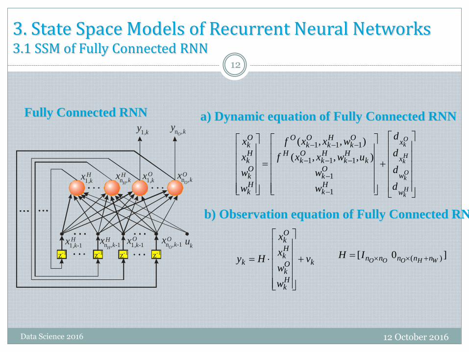
3. State Space Models of Recurrent Neural Networks3.1 SSM of Fully Connected RNN

y y1,k n ,k

uk

H

H

H

H

O

O

O

O

z-1 z-1 z-1 z-1

x1, -1k

x1,k

x1, -1k

x1,k

xn , -1k

H

xn ,k

H

x

x

n , -1k

n ,k

O

O

O

Hk

Ok

Hk

Ok

w

w

x

x

Hk

Ok

kHk

Hk

Ok

H

Ok

Hk

Ok

O

Hk

Ok

Hk

Ok

d

d

d

d

w

w

uwxxf

wxxf

w

w

x

x

1

1

111

111

),,,(

),,(

k

Hk

Ok

Hk

Ok

k v

w

w

x

x

Hy

]0[ )( WHOOO nnnnnIH


b) Observation equation of Fully Connected RNN

a) Dynamic equation of Fully Connected RNNFully Connected RNN

13

x

xx

H

OO

H

H

H

H

H

x x1,k

1,k

2,k n ,k

n ,k

H

uk

z-1 z-1 z-1

x x x1,k-1 2,k-1 n ,k-1H

O

Hk

Ok

Hk

w

w

x

Hk

Ok

kHk

Hk

Hk

Ok

Hk

d

d

d

w

w

uwxf

w

w

x

1

1

11 ),,(

kOk

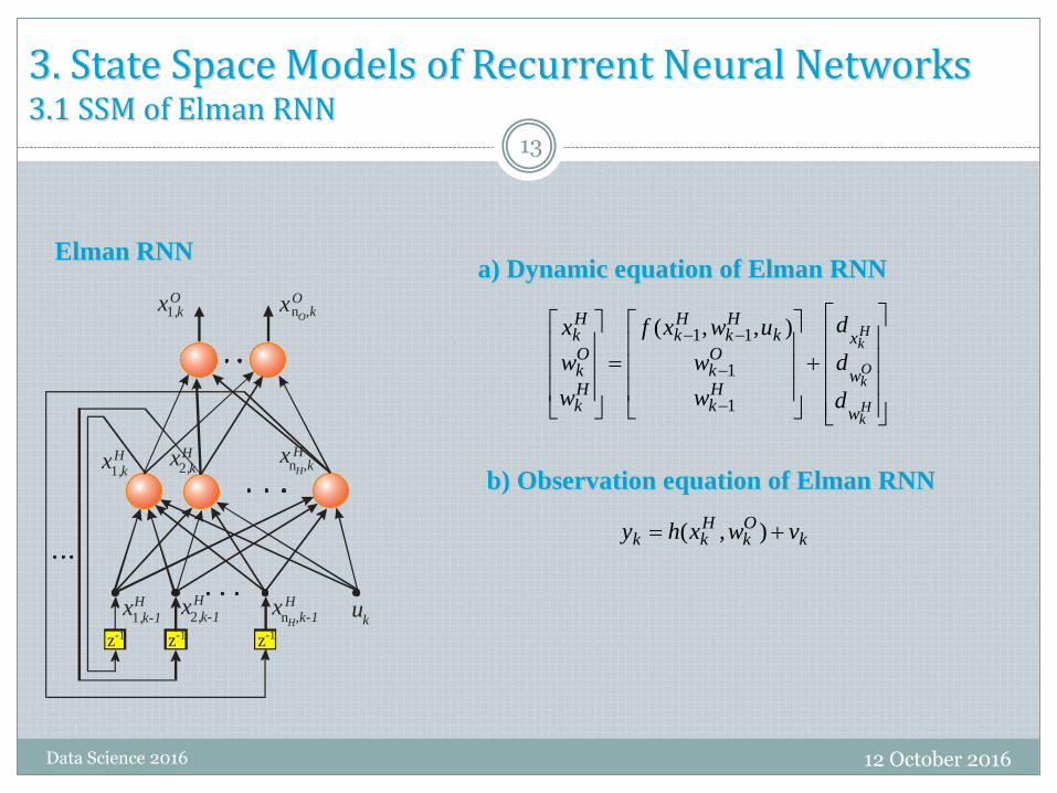
Hkk vwxhy ),(


b) Observation equation of Elman RNN

a) Dynamic equation of Elman RNNElman RNN

3. State Space Models of Recurrent Neural Networks3.1 SSM of Elman RNN

14

3. State Space Models of Recurrent Neural Networks3.3 SSM of NARX RNN

xkO

O O

z-1 z-1z-1z-1

uu

xk-1

uk-1kx

k-u

xk-

Hk

Ok

Ok

x

ux

x

w

w

x

Hk

Ok

Ok

Ok

kkkOk

Ok

Hk

Ok

Ok

Ok

Ok

d

d

d

w

w

x

x

wuuxxf

w

w

x

x

x

0

0

),,..,,,..,(

1

1

1

1

111

1

1

k

Hk

Ok

Ok

Ok

Ok

k v

w

w

x

x

x

Hy

x

1

1



b) Observation equation of NARX RNN

a) Dynamic equation of NARX RNN

Nonlinear AutoRegressive

Exogenous (NARX) RNN

15

Okw

Ok

Ok dww 1

kOk

T

Rk

kOkk vw

x

uxy

1


b) Observation equation of ECHO state RNN

a) Dynamic equation of ECHO state RNN

ECHO state RNN

1z 1z 1z

Rkx 1,

Rkx 2,

Rnk R

x ,

Rkx 1,1

Rkx 2,1

Rnk R

x ,1

Okx

ku

k

IRRk

RRk

Rk u

WxWaxax1

tanh)1( 11

Fixed random weights

(usually sparse connectivity)

3. State Space Models of Recurrent Neural Networks3.1 SSM of ECHO state RNN

16

3. State Space Models of Recurrent Neural Networks3.3 SSM of ECHO state RNN with Teacher Leading (ECHO TL)

Hk

Ok

Ok

x

ux

w

w

x

Hk

Ok

Ok

Ok

kkkOk

Ok

d

d

d

w

w

x

x

wuuxxf

0

0

),,..,,,..,(

1

1

1

1

111

k

Hk

Ok

Ok

Ok

Ok

k v

w

w

x

x

x

Hy

x

1

1



b) Observation equation of ECHO TL RNN

a) Dynamic equation of ECHO TL RNN

ECHO TL RNN

1z 1z 1zRkx 1,

Rkx 2,

R

nk Rx,

Rkx 1,1

Rkx 2,1

R

nk Rx,1

Okx 1,

1z

Rkx 1,1

Rkx 2,1

R

nk Rx,1

Okx 1,1

ku


(usually sparse connectivity)


OUTLINE





5. Examples

18

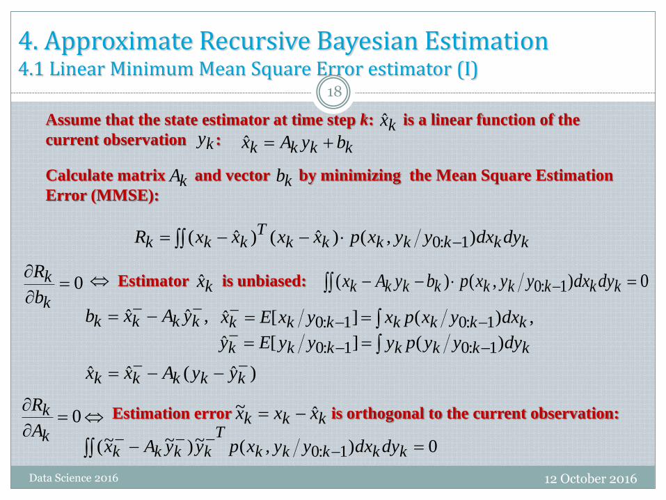
4. Approximate Recursive Bayesian Estimation4.1 Linear Minimum Mean Square Error estimator (I)


Assume that the state estimator at time step k: is a linear function of the

current observation :

Calculate matrix and vector by minimizing the Mean Square Estimation

Error (MMSE):

kkkk byAx ˆkx

ky

kA kb

kkkkkkkT

kkk dydxyyxpxxxxR ),()ˆ()ˆ( 1:0

0

k

k

b

R Estimator is unbiased:kx 0),()( 1:0 kkkkkkkkk dydxyyxpbyAx

0

k

k

A

R Estimation error is orthogonal to the current observation:

,ˆˆ kkkk yAxb ,)(][ˆ 1:01:0 kkkkkkk dxyxpxyxEx

kkkkkkk dyyypyyyEy )(][ˆ 1:01:0

0),(~)~~( 1:0 kkkkk

T

kkkk dydxyyxpyyAx

)ˆ(ˆˆ kkkkk yyAxx

kkk xxx ˆ~

19

4. Approximate Recursive Bayesian Estimation4.1 Linear Minimum Mean Square Error estimator (II)

1. PredictionGiven the state estimate and associated covariance at time step k-1:

),ˆ(11 kxk Px

a) Predict new state and associated covariance:

),,( 1 kkkkk duxfx

b) Predict the expected observation and associated covariance:

),( kkkk vxhy

c) Predict the cross-correlation matrix of state and observation:

kkkkkkkkk dddxdpyxpduxfx 11:011 )()(),,(ˆ

kkkkk

Tkkkkkkkkx

dvdxdpyxp

xduxfxduxfPk

11:01

11

)()(

)ˆ),,()(ˆ),,((

kkkkkkkk dvdxvpyxpvxhy )()(),(ˆ 1:0

kkkkk

Tkkkkkky dvdxvpyxpyvxhyvxhP

k)()()ˆ),()(ˆ),(( 1:0

12 October 2016NCTA 2014

kkkkkT

kkkkkyx dvdxvpyxpyvxhxxPkk

)()()ˆ),()(ˆ( 1:0


20

4. Approximate Recursive Bayesian Estimation4.1 Linear Minimum Mean Square Error estimator (III)

1. PredictionGiven the state estimate and associated covariance at time step k-1:

),ˆ(11 kxk Px

a) Predict new state and associated covariance:

),,( 1 kkkkk duxfx

b) Predict the expected observation and associated covariance:

),( kkkk vxhy

c) Predict the cross-correlation matrix of state and observation:

12 October 2016NCTA 2014

),ˆ(11 kxk Px

),ˆ(11 kyk Py

2. UpdateThe state estimate and associated covariance at time step k:

)ˆ()(ˆˆ 1 kkyyxkk yyPPxxkkk

kkkkkkk xyyyxxx PPPPP 1)(

kk yxP


4. Approximate Recursive Bayesian Estimation4.2 Propagating random variable through nonlinear mapping


21

a) Linear approximation of Taylor series expansion – Extended

Kalman Filter (EKF )[Anderson, B. and J. Moore

))(()()( xxxfxfxf

b) Stirling’s interpolation formula – Divided Difference Kalman

Filter (DDKF) [Nørgaard et al., 2000]

c) Unscented transform – Unscented Kalman Filter (UKF)[Julier and

Uhlmann, 1997]

2)(!2

)())(()()( xx

xfxxxfxfxf DD

DD

)(, 00 nx

ninPnx iixi ,...,2,1,)(5.0,))((

niknPnx niixni ,...,2,1,)(5.0,))((

h

hxfhxfxfDD

)()()(

2

)(2)()()(

h

xfhxfhxfxfDD

The n-dimensional random variable is approximated

by a set of 2n+1 deterministically selected points:

),(~ xPxx

c) Noise models (UNKNOWN):

b) Exact analytical forms of the dynamics and the observation

process (UNKNOWN):

4. Approximate Recursive Bayesian Estimation of the

Recurrent Neural Network state22


What is known?

a) Sequences of inputs and observations: ),( :0:0 kk yu

kk hf ,

)(),( kk vpdp

What should be estimated?

Estimate recursively probability density function (pdf) of the state :

given the input and

the observation sequence .

kx

?)( :0 kk yxp

Each sample is presented to the RNN and learning algorithm

only once.

,...}1,0,{:0 kuu kk

,...}1,0,{:0 kyy kk

),( kk yu


OUTLINE





5. Examples

5. Examples


24

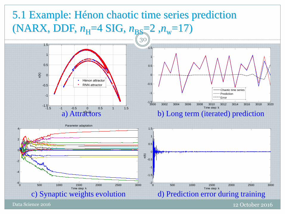
After sequential training on certain number of samples, recurrent neural

networks were iterated for a number of samples, by feeding back just the

predicted outputs as the new inputs of the recurrent neurons.

Time series of N iterated predictions were compared with the test parts of the

original time series by calculating the Normalized Root Mean Squared Error

(NRMSE):

σ is the standard deviation of chaotic time series;

N

kkk

NyyNRMSE

1

21 )ˆ(2

yk is the true value of sample at time step k, and is the RNN prediction.ky

5.1 Example: Hénon chaotic time series prediction


25

22

1 3.04.11 kkk xxx

Hénon difference equation

a) Hénon attractor b) Hénon time series

0 500 1000 1500 2000 2500 3000-2

-1.5

-1

-0.5

0

0.5

1

1.5

Time step: k

e(k

)

3000 3002 3004 3006 3008 3010 3012 3014 3016 3018 3020-1.5

-1

-0.5

0

0.5

1

1.5

Time step: k

Chaotic time series

Prediction

Error

0 500 1000 1500 2000 2500 3000-15

-10

-5

0

5

10

15Parameter adaptation

Time step: k

-1.5 -1 -0.5 0 0.5 1 1.5-1.5

-1

-0.5

0

0.5

1

1.5

x(k-1)

x(k

)

Hénon attractor

RNN attractor


(ELMAN, DDF, nH=4 SIG, nBS=4, nw=25)


26

c) Synaptic weights evolution d) Prediction error during training

a) Attractors b) Long term (iterated) prediction


0 500 1000 1500 2000 2500 3000-2

-1.5

-1

-0.5

0

0.5

1

1.5

Time step: k

e(k

)

3000 3002 3004 3006 3008 3010 3012 3014 3016 3018 3020-1.5

-1

-0.5

0

0.5

1

1.5

Time step: k

Chaotic time series

Prediction

Error

0 500 1000 1500 2000 2500 3000-15

-10

-5

0

5

10


Time step: k

-1.5 -1 -0.5 0 0.5 1 1.5-1.5

-1

-0.5

0

0.5

1

1.5

x(k-1)

x(k

)

Hénon attractor

RNN attractor


(ELMAN, DDF, nH=4 SIG, nBS=4, nw=25)


27


x

xx

H

OO

H

H

H

H

H

x x1,k

1,k

2,k n ,k

n ,k

H

uk

z-1 z-1 z-1

x x x1,k-1 2,k-1 n ,k-1H

O

-1.5 -1 -0.5 0 0.5 1 1.5-1.5

-1

-0.5

0

0.5

1

1.5

x(k-1)

x(k

)

Hénon attractor

RNN attractor

3000 3002 3004 3006 3008 3010 3012 3014 3016 3018 3020-2

-1.5

-1

-0.5

0

0.5

1

1.5

Time step: k

Chaotic time series

Prediction

Error

0 500 1000 1500 2000 2500 3000-2

-1.5

-1

-0.5

0

0.5

1

1.5

Time step: k

e(k

)

0 500 1000 1500 2000 2500 3000-10

-5

0

5

10


Time step: k


(ELMAN, DDF, nH=3 RBF, nBS=3, nw=22)


28



-1.5 -1 -0.5 0 0.5 1 1.5-1.5

-1

-0.5

0

0.5

1

1.5

x(k-1)

x(k

)

Hénon attractor

RNN attractor

3000 3002 3004 3006 3008 3010 3012 3014 3016 3018 3020-2

-1.5

-1

-0.5

0

0.5

1

1.5

Time step: k

Chaotic time series

Prediction

Error

0 500 1000 1500 2000 2500 3000-2

-1.5

-1

-0.5

0

0.5

1

1.5

Time step: k

e(k

)

0 500 1000 1500 2000 2500 3000-10

-5

0

5

10


Time step: k


29



x

xx

H

OO

H

H

H

H

H

x x1,k

1,k

2,k n ,k

n ,k

H

uk

z-1 z-1 z-1

x x x1,k-1 2,k-1 n ,k-1H

O


(ELMAN, DDF, nH=3 RBF, nBS=3, nw=22)

3000 3002 3004 3006 3008 3010 3012 3014 3016 3018 3020-1.5

-1

-0.5

0

0.5

1

1.5

Time step: k

Chaotic time series

Prediction

Error

0 500 1000 1500 2000 2500 3000-6

-4

-2

0

2


Time step: k0 500 1000 1500 2000 2500 3000

-2

-1.5

-1

-0.5

0

0.5

1

1.5

Time step: k

e(k

)

-1.5 -1 -0.5 0 0.5 1 1.5-1.5

-1

-0.5

0

0.5

1

1.5

x(k-1)

x(k

)

Hénon attractor

RNN attractor


(NARX, DDF, nH=4 SIG, nBS=2 ,nw=17)


30



3000 3002 3004 3006 3008 3010 3012 3014 3016 3018 3020-1.5

-1

-0.5

0

0.5

1

1.5

Time step: k

Chaotic time series

Prediction

Error

0 500 1000 1500 2000 2500 3000-6

-4

-2

0

2


Time step: k0 500 1000 1500 2000 2500 3000

-2

-1.5

-1

-0.5

0

0.5

1

1.5

Time step: k

e(k

)

-1.5 -1 -0.5 0 0.5 1 1.5-1.5

-1

-0.5

0

0.5

1

1.5

x(k-1)

x(k

)

Hénon attractor

RNN attractor


(NARX, DDF, nH=4 SIG, nBS=2 ,nw=17)


31



xkO

O O

z-1 z-1z-1z-1

uu

xk-1

uk-1kx

k-u

xk-

0 500 1000 1500 2000 2500 3000-2

-1.5

-1

-0.5

0

0.5

1

1.5

Time step: k

e(k

)

-1.5 -1 -0.5 0 0.5 1 1.5-1.5

-1

-0.5

0

0.5

1

1.5

x(k-1)

x(k

)

Hénon attractor

RNN attractor

3000 3002 3004 3006 3008 3010 3012 3014 3016 3018 3020-1.5

-1

-0.5

0

0.5

1

1.5

Time step: k

Chaotic time series

Prediction

Error

0 500 1000 1500 2000 2500 3000-30

-20

-10

0

10

20


Time step: k


(NARX, DDF, nH=3 RBF, nBS=2, nw=16)


32



0 500 1000 1500 2000 2500 3000-2

-1.5

-1

-0.5

0

0.5

1

1.5

Time step: k

e(k

)

-1.5 -1 -0.5 0 0.5 1 1.5-1.5

-1

-0.5

0

0.5

1

1.5

x(k-1)

x(k

)

Hénon attractor

RNN attractor

3000 3002 3004 3006 3008 3010 3012 3014 3016 3018 3020-1.5

-1

-0.5

0

0.5

1

1.5

Time step: k

Chaotic time series

Prediction

Error

0 500 1000 1500 2000 2500 3000-30

-20

-10

0

10

20


Time step: k


(NARX, DDF, nH=3 RBF, nBS=2, nw=16)


33



xkO

O O

z-1 z-1z-1z-1

uu

xk-1

uk-1kx

k-u

xk-

34


Hn


Mean Var T[s]

DDF_ELMAN_SIG 1.73e-2 6.19e-5 4 25 8.34

DDF_ELMAN_RBF 6.02e-2 3.89e-4 3 22 7.76

UKF_ELMAN_SIG 7.29e-2 9.46e-3 4 25 8.53

UKF_ELMAN_RBF 7.24e-2 1.79e-3 3 22 7.91

EKF_ELMAN_SIG 1.69e-1 5.17e-2 4 25 7.69

EKF_ELMAN_RBF 1.01e-1 7.50e-3 3 22 7.96

DDF_NARX_SIG 7.46e-3 3.39e-6 4 17 6.21

DDF_NARX_RBF 4.36e-3 4.15e-6 3 16 5.85

UKF_NARX_SIG 1.28e-2 2.68e-5 4 17 6.37

UKF_NARX_RBF 5.72e-3 7.14e-6 3 16 6.00

EKF_NARX_SIG 1.57e-2 1.65e-5 4 17 5.76

EKF_NARX_RBF 7.07e-3 1.35e-6 3 16 6.17

Wn

5.2 Example: Mackey-Glass( ) chaotic time series

long term prediction


35

Chaotic time series is obtained from the Mackey-Glass equation

10)(1

)()()(

tx

taxtbxtx

which exhibits chaotic behaviour for ,2.0a ,1.0b 17

Equation is integrated using fourth-order Runge-Kutta method with

an integration time step 0.01. The resulting time series is sampled at

1 Hz to obtain a sequence of 3000 training samples and 3000 test

samples for clean (1000 test samples for noisy time series).

17

5.2 Example: Mackey-Glass( ) chaotic time series long term

prediction: ECHO TL (500 RN-s, 2% conn.)


36

0 500 1000 1500 2000 2500 3000-0.6

-0.4

-0.2

0

0.2

0.4

Time steps: k

Iterated prediction of Mackey-Glass(tau = 17) time series

Original

Prediction

0 500 1000 1500 2000 2500 3000-0.5

-0.4

-0.3

-0.2

-0.1

0

0.1

0.2

0.3

0.4Long term predicton error of Mackey-Glass(tau = 17) time series

Time steps: k

17


prediction: ECHO TL (500 RN-s, 2% conn.)


37

0 500 1000 1500 2000 2500 3000-0.6

-0.4

-0.2

0

0.2

0.4

Time steps: k


Original

Prediction

0 500 1000 1500 2000 2500 3000-0.5

-0.4

-0.3

-0.2

-0.1

0

0.1

0.2

0.3


Time steps: k

17

1z 1z 1zRkx 1,

Rkx 2,

R

nk Rx,

Rkx 1,1

Rkx 2,1

R

nk Rx,1

Okx 1,

1z

Rkx 1,1

Rkx 2,1

R

nk Rx,1

Okx 1,1

ku


(usually sparse

connectivity)


prediction: (NARX, SRKF, nH=8 SIG, nBS=5 ,nw=54)


38

17

500 1000 1500 2000 2500 3000-0.8

-0.6

-0.4

-0.2

0

0.2

0.4

0.6


Time steps: k

0 500 1000 1500 2000 2500 30000.4

0.6

0.8

1

1.2

1.4

Time steps: k


Original

Prediction




39

17

500 1000 1500 2000 2500 3000-0.8

-0.6

-0.4

-0.2

0

0.2

0.4

0.6


Time steps: k

0 500 1000 1500 2000 2500 30000.4

0.6

0.8

1

1.2

1.4

Time steps: k


Original

Prediction

xkO

O O

z-1 z-1z-1z-1

uu

xk-1

uk-1kx

k-u

xk-

5.3 Example: Noisy Mackey-Glass( ) chaotic time series long

term prediction: ECHO TL (500 RN-s, 2% conn.)


40

17

100 200 300 400 500 600 700 800 900 1000-0.8

-0.6

-0.4

-0.2

0

0.2

0.4

0.6


Time steps: k

0 100 200 300 400 500 600 700 800 900 1000-0.8

-0.6

-0.4

-0.2

0

0.2

0.4

0.6

0.8

Time steps: k


Noisy

Original

Prediction

5.3 Example: Noisy Mackey-Glass( ) chaotic time series long

term prediction: ECHO TL (500 RN-s, 2% conn.)


41

17

100 200 300 400 500 600 700 800 900 1000-0.8

-0.6

-0.4

-0.2

0

0.2

0.4

0.6


Time steps: k

0 100 200 300 400 500 600 700 800 900 1000-0.8

-0.6

-0.4

-0.2

0

0.2

0.4

0.6

0.8

Time steps: k


Noisy

Original

Prediction

1z 1z 1zRkx 1,

Rkx 2,

R

nk Rx,

Rkx 1,1

Rkx 2,1

R

nk Rx,1

Okx 1,

1z

Rkx 1,1

Rkx 2,1

R

nk Rx,1

Okx 1,1

ku


(usually sparse

connectivity)




42

17

0 100 200 300 400 500 600 700 800 900 10000

0.2

0.4

0.6

0.8

1

1.2

1.4

1.6

1.8

Time steps: k

Iterated prediction of noisy Mackey-Glass(tau = 17) time series (SNR = 1dB)

Noisy

Original

Prediction

100 200 300 400 500 600 700 800 900 1000-0.4

-0.2

0

0.2

0.4

0.6

0.8

1

1.2

1.4Long term predicton error of noisy Mackey-Glass(tau = 17) time series (SNR = 1dB)

Time steps: k

100 200 300 400 500 600 700 800 900 1000-0.4

-0.2

0

0.2

0.4

0.6

0.8

1

1.2

1.4Long term predicton error of noisy Mackey-Glass(tau = 17) time series (SNR = 1dB)

Time steps: k




43

17

0 100 200 300 400 500 600 700 800 900 10000

0.2

0.4

0.6

0.8

1

1.2

1.4

1.6

1.8

Time steps: k

Iterated prediction of noisy Mackey-Glass(tau = 17) time series (SNR = 1dB)

Noisy

Original

Prediction

xkO

O O

z-1 z-1z-1z-1

uu

xk-1

uk-1kx

k-u

xk-

44

6. Conclusions


HnWn

ECHO state recurrent neural network and NARX recurrent neural network

belong to the class of Reservoir Computing recurrent neural networks.

ECHO state RNN has reservoir of nonlinear recurrent neurons and linear

readout layer.

NARX RNN has reservoir of linear neurons and nonlinear readout layers.

Both networks have fast learning and superior generalization capabilities,

compared to the other RNN architectures.

Appendix: Approximate nonlinear non-Gaussian

estimation


45

PxxNwAyxpyAPyxp jxjkk

n

j,jkjkkk

n

jkjkkk k

kk

),ˆ;( ),(}{)( ,,111

1,11:011

1:0,11:01 1

11

QddNwdBdpBPdp ikikk

n

jk,iikk

n

jjkk

kdkd

),;( )(}{)( ,,1

,1

,

RvvNwvCvpCPvp ikikk

n

jk,iikk

n

jjkk

kvkv

),;( )(}{)( ,,1

,1

,

State pdf in k-1

Process noise pdf

Observation noise pdf

-25 -20 -15 -10 -5 0 5 10 15 20 250

0.05

0.1

0.15

0.2

0.25

Gaussian Sum filters – applying mixtures of Gaussians to approximate non-

Gaussian pdf’s.

Appendix: Approximate nonlinear non-Gaussian

estimation


46

PxxNwAyxpyAPyxp jxjkk

n

j,jkjkkk

n

jkjkkk k

kk

),ˆ;( ),(}{)( ,,111

1,11:011

1:0,11:01 1

11

QddNwdBdpBPdp ikikk

n

jk,iikk

n

jjkk

kdkd

),;( )(}{)( ,,1

,1

,

RvvNwvCvpCPvp ikikk

n

jk,iikk

n

jjkk

kvkv

),;( )(}{)( ,,1

,1

,

State pdf in k-1

Process noise pdf

Observation noise pdf

-25 -20 -15 -10 -5 0 5 10 15 20 250

0.05

0.1

0.15

0.2

0.25

-25 -20 -15 -10 -5 0 5 10 15 20 250

0.05

0.1

0.15

0.2

0.25

Gaussian Sum filters – applying mixtures of Gaussians to approximate non-

Gaussian pdf’s.

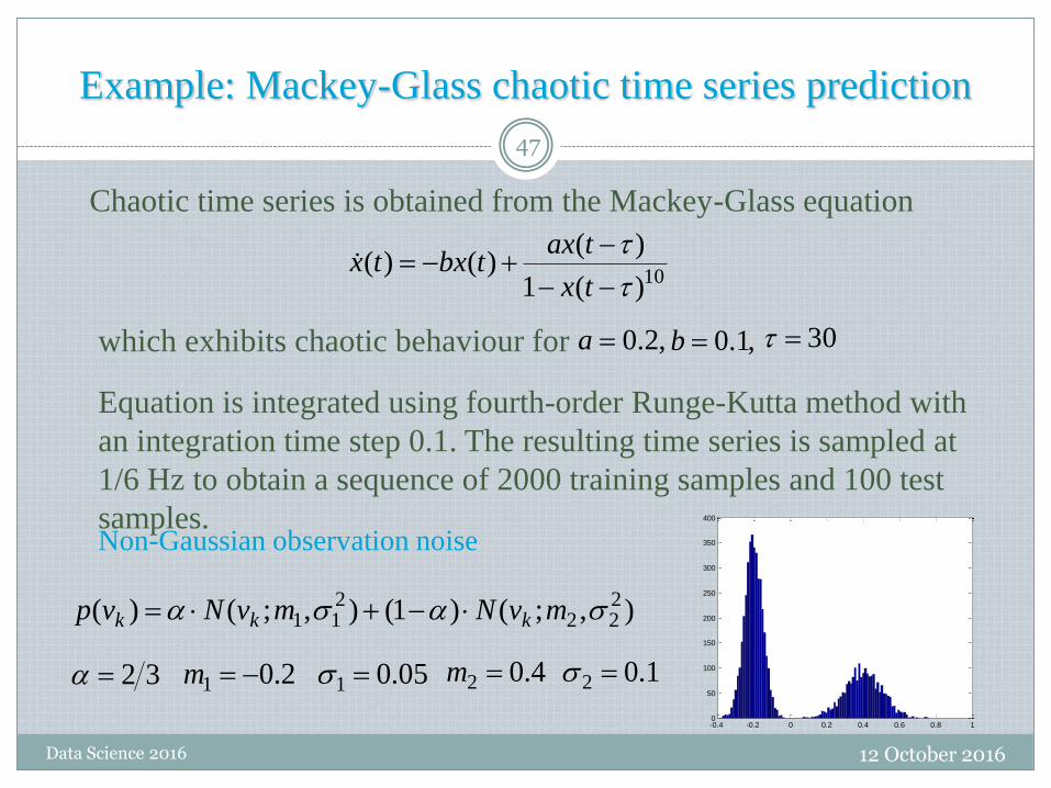
Example: Mackey-Glass chaotic time series prediction


47

Chaotic time series is obtained from the Mackey-Glass equation

10)(1

)()()(

tx

taxtbxtx

which exhibits chaotic behaviour for ,2.0a ,1.0b 30

Equation is integrated using fourth-order Runge-Kutta method with

an integration time step 0.1. The resulting time series is sampled at

1/6 Hz to obtain a sequence of 2000 training samples and 100 test

samples.

-0.4 -0.2 0 0.2 0.4 0.6 0.8 10

50

100

150

200

250

300

350

400

),;()1(),;()( 222

211 mvNmvNvp kkk

Non-Gaussian observation noise

32 2.01 m 05.01 4.02 m 1.02


48

00.5

11.5

0

0.5

1

1.50

0.5

1

1.5

x(k-1)

Mackey Glass atraktor

x(k-2)

x(k

)

00.5

11.5

2

0

1

20

0.5

1

1.5

2

x(k-1)

Noisy Mackey Glass atraktor

x(k-2)x(k

)

00.5

11.5

0

0.5

1

1.50

0.5

1

1.5

x(k-1)

Atraktor NARX RMLP mre e

x(k-2)

x(k

)

2010 2020 2030 2040 2050 2060 2070 2080 2090 2100-0.5

0

0.5

1

1.5

2

2.5NARX RMLP iterisana predikcija Mackey-Glass haoti~ne serije

Korak diskretizacije vremena: k

Haoti~na serija naru{ena {umomHaoti~na serijaPredikcijaGre{ka

0 200 400 600 800 1000 1200 1400 1600 1800 20000

0.2

0.4

0.6

0.8

1Verovatno}e komponenti sume Gausijana

Korak diskretizacije vremena: k

P(Ak,1

/y0:k

)

P(Ak,2

/y0:k

)

P(Ak,3

/y0:k

)

0 5 10 15 20 25 30 35 40 45 50-2

-1.5

-1

-0.5

0

0.5

1

1.5

2xk,1

=E[xk/y

0:k,A

k,1]

xk,2

=E[xk/y

0:k,A

k,2]

xk,3

=E[xk/y

0:k,A

k,3]

a) Mackey-Glass attractor b) Noisy attractor c) RNN reconstructed attractor

d) Long term prediction e) Component probabilities f) Final weights

Example: Mackey-Glass chaotic time series prediction - multimodal

noise case (GS_DDF, nH=5 SIG, nBS=6, nw=41, n=3 components)

Data & Analytics

Recursive Bayesian estimation of ECHO state recurrent neural networks - Branimir Todorovic