Embed Size (px)
Citation preview
Analysis of Factors affecting Net Profit of ONGC
Submitted By => KARAN SHAH Enrollment No. => 1011517039 Date => 06/09/2016 Submitted To => Dr. Abhay Raja
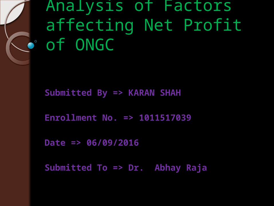
Objective of the StudyThe objective of this study is to
analyze the impact of Sales, Interest Exp. and Average Oil Prices (USD/barrel) on the Quarterly net profits of ONGC. Also, to study whether each quarter significantly impacts the Net Profit of the company.
Identifying Dependent and Independent Variable
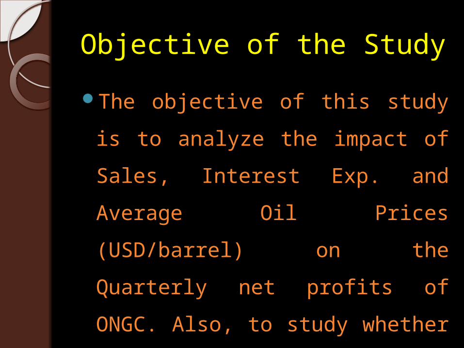
Dependent Variable: - Net Profit after Tax of ONGC for last 15 Quarters
Independent Variables:- Sales, Interest Exp. and Average Oil Prices (USD/barrel)
Dummy Variables:- Q1, Q2, Q3 and Q4

Analysis Using E-views
Software
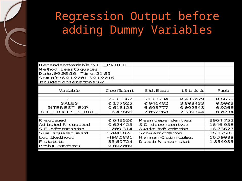
Regression Output before adding Dummy Variables
Dependent Variable: NET_PROFITMethod: Least SquaresDate: 09/05/16 Time: 21:59Sample: 6/01/2001 3/01/2016Included observations: 60
Variable Coefficient Std. Error t-Statistic Prob.
C 223.3362 513.3234 0.435079 0.6652SALES 0.177025 0.046482 3.808433 0.0003
INTEREST_EXP_ -0.618125 6.693777 -0.092343 0.9268OIL_PRICES_$_BBL_ 16.43866 7.052968 2.330744 0.0234
R-squared 0.643520 Mean dependent var 3964.752Adjusted R-squared 0.624423 S.D. dependent var 1646.938S.E. of regression 1009.314 Akaike info criterion 16.73627Sum squared resid 57048076 Schwarz criterion 16.87589Log likelihood -498.0881 Hannan-Quinn criter. 16.79088F-statistic 33.69724 Durbin-Watson stat 1.854935Prob(F-statistic) 0.000000
InterpretationFrom the above output as we can
see that significance level of “Interest Expense” is 0.9268, which is greater than 0.05, which means that “Interest Expense” is not significant in predicting the Net Profit of ONGC. So, we remove the interest expense and the output is given in the next slide.
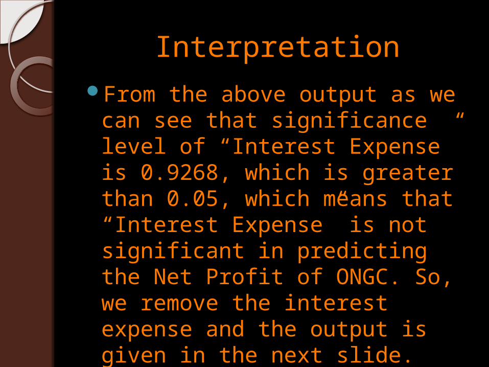
Dependent Variable: NET_PROFITMethod: Least SquaresDate: 09/05/16 Time: 22:02Sample: 6/01/2001 3/01/2016Included observations: 60
Variable Coefficient Std. Error t-Statistic Prob.
C 195.6652 413.1428 0.473602 0.6376SALES 0.178715 0.042355 4.219452 0.0001
OIL_PRICES_$_BBL_ 16.34077 6.911926 2.364141 0.0215
R-squared 0.643466 Mean dependent var 3964.752Adjusted R-squared 0.630956 S.D. dependent var 1646.938S.E. of regression 1000.498 Akaike info criterion 16.70309Sum squared resid 57056763 Schwarz criterion 16.80781Log likelihood -498.0927 Hannan-Quinn criter. 16.74405F-statistic 51.43629 Durbin-Watson stat 1.850975Prob(F-statistic) 0.000000
As we can see the significance levels of Sales and Avg. Oil Prices (USD/Barrel) have changed but still they significantly impact the Net Profit of ONGC.
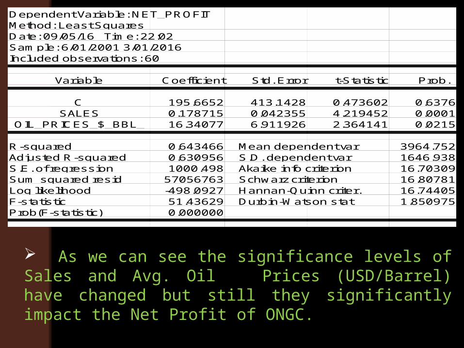
Regression Output after adding Dummy Variables
As we can see that even after adding dummy variables “Interest Exp.” is not significant
Dependent Variable: NET_PROFITMethod: Least SquaresDate: 09/05/16 Time: 22:08Sample: 6/01/2001 3/01/2016Included observations: 60
Variable Coefficient Std. Error t-Statistic Prob.
C 247.1278 514.1621 0.480642 0.6327SALES 0.172291 0.043671 3.945242 0.0002
INTEREST_EXP_ 0.511423 6.353854 0.080490 0.9362OIL_PRICES_$_BBL_ 17.15152 6.628872 2.587397 0.0124
DUMMY_QRT_1 -631.7632 345.4176 -1.828984 0.0730DUMMY_QRT_2 11.05170 347.8075 0.031775 0.9748DUMMY_QRT_3 552.5482 346.0343 1.596802 0.1163
R-squared 0.709052 Mean dependent var 3964.752Adjusted R-squared 0.676114 S.D. dependent var 1646.938S.E. of regression 937.2884 Akaike info criterion 16.63314Sum squared resid 46561007 Schwarz criterion 16.87748Log likelihood -491.9942 Hannan-Quinn criter. 16.72871F-statistic 21.52714 Durbin-Watson stat 1.800765Prob(F-statistic) 0.000000
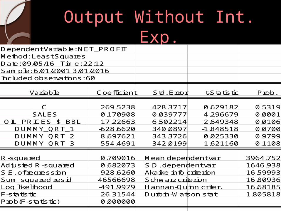
Output Without Int. Exp.Dependent Variable: NET_PROFITMethod: Least SquaresDate: 09/05/16 Time: 22:12Sample: 6/01/2001 3/01/2016Included observations: 60
Variable Coefficient Std. Error t-Statistic Prob.
C 269.5238 428.3717 0.629182 0.5319SALES 0.170908 0.039777 4.296679 0.0001
OIL_PRICES_$_BBL_ 17.22663 6.502214 2.649348 0.0106DUMMY_QRT_1 -628.6620 340.0897 -1.848518 0.0700DUMMY_QRT_2 8.697621 343.3726 0.025330 0.9799DUMMY_QRT_3 554.4691 342.0199 1.621160 0.1108
R-squared 0.709016 Mean dependent var 3964.752Adjusted R-squared 0.682073 S.D. dependent var 1646.938S.E. of regression 928.6260 Akaike info criterion 16.59993Sum squared resid 46566698 Schwarz criterion 16.80936Log likelihood -491.9979 Hannan-Quinn criter. 16.68185F-statistic 26.31544 Durbin-Watson stat 1.805818Prob(F-statistic) 0.000000
Interpretation of the Output
As we can see the probability values of all the dummy variables are
greater than 0.05, which means all the dummy variables are
insignificant at 95% confidence level.
Hence, we can say that with the change in quarter of a year, the net
profit of ONGC does not get impacted significantly or else we can say
that net profit is not dependent on the quarter of a year.
Also, with the addition of dummy variables the other independent
variables (Sales and Oil Prices) remain significant.
Regression Equation
Net Profit = 269.52+0.1709(Sales) + 17.2266(Oil Prices USD/bbl) - 628.662(Q1Profit) + 8.697
(Q2 Profit) + 4.4691(Q3 Profit)

Testing the Assumptions of CLRM
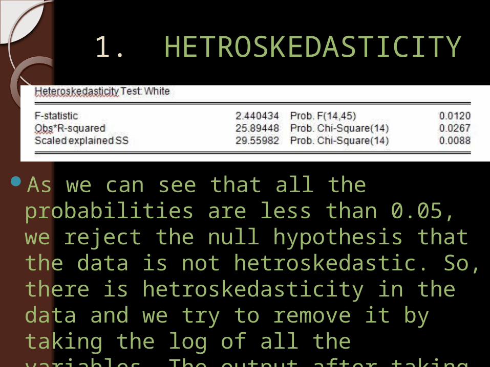
1. HETROSKEDASTICITY
As we can see that all the probabilities are less than 0.05, we reject the null hypothesis that the data is not hetroskedastic. So, there is hetroskedasticity in the data and we try to remove it by taking the log of all the variables. The output after taking log is given in next slide.
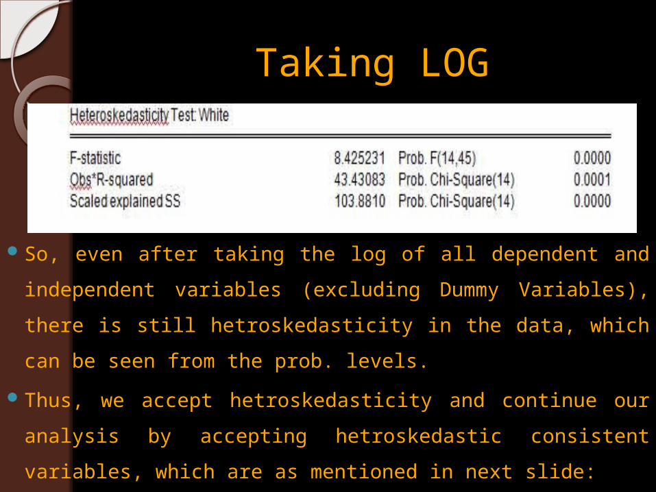
Taking LOG
So, even after taking the log of all dependent and independent variables (excluding Dummy Variables), there is still hetroskedasticity in the data, which can be seen from the prob. levels.
Thus, we accept hetroskedasticity and continue our analysis by accepting hetroskedastic consistent variables, which are as mentioned in next slide:
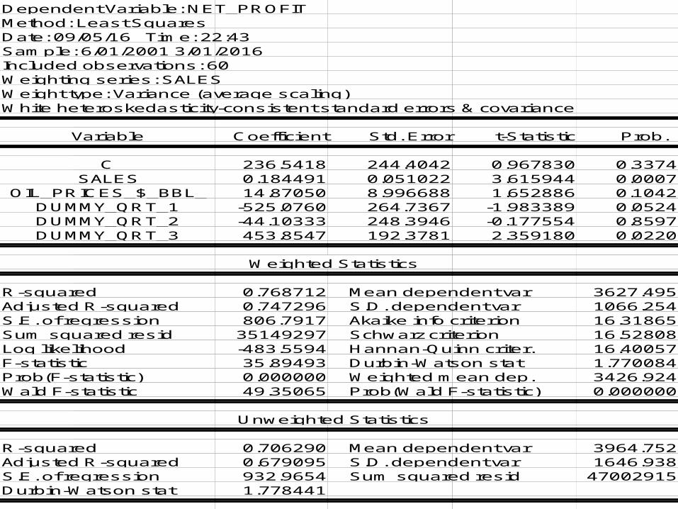
Dependent Variable: NET_PROFITMethod: Least SquaresDate: 09/05/16 Time: 22:43Sample: 6/01/2001 3/01/2016Included observations: 60Weighting series: SALESWeight type: Variance (average scaling)White heteroskedasticity-consistent standard errors & covariance
Variable Coefficient Std. Error t-Statistic Prob.
C 236.5418 244.4042 0.967830 0.3374SALES 0.184491 0.051022 3.615944 0.0007
OIL_PRICES_$_BBL_ 14.87050 8.996688 1.652886 0.1042DUMMY_QRT_1 -525.0760 264.7367 -1.983389 0.0524DUMMY_QRT_2 -44.10333 248.3946 -0.177554 0.8597DUMMY_QRT_3 453.8547 192.3781 2.359180 0.0220
Weighted Statistics
R-squared 0.768712 Mean dependent var 3627.495Adjusted R-squared 0.747296 S.D. dependent var 1066.254S.E. of regression 806.7917 Akaike info criterion 16.31865Sum squared resid 35149297 Schwarz criterion 16.52808Log likelihood -483.5594 Hannan-Quinn criter. 16.40057F-statistic 35.89493 Durbin-Watson stat 1.770084Prob(F-statistic) 0.000000 Weighted mean dep. 3426.924Wald F-statistic 49.35065 Prob(Wald F-statistic) 0.000000
Unweighted Statistics
R-squared 0.706290 Mean dependent var 3964.752Adjusted R-squared 0.679095 S.D. dependent var 1646.938S.E. of regression 932.9654 Sum squared resid 47002915Durbin-Watson stat 1.778441
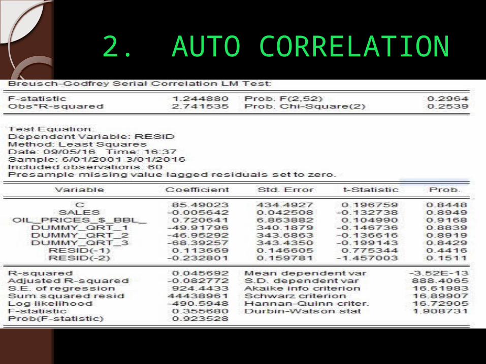
2. AUTO CORRELATION
Interpretation
All the prob. levels are greater than 0.05, hence we accept the null hypothesis that “there is no auto correlation between the observations”. Hence, this assumption of CLRM is fulfilled.
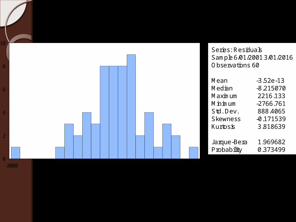
3. TEST OF NORMALITY
0
2
4
6
8
10
-3000 -2000 -1000 0 1000 2000
Series: ResidualsSample 6/01/2001 3/01/2016Observations 60
Mean -3.52e-13Median -8.215070Maximum 2216.133Minimum -2766.761Std. Dev. 888.4065Skewness -0.171539Kurtosis 3.818639
Jarque-Bera 1.969682Probability 0.373499
InterpretationTo test the normality of the data, we use Jarque –
Bera test. Here, the prob. of Jarque Bera is 0.3734, which is greater than 0.05, hence we reject the null hypothesis that “data is not normal”.
The Kurtosis Value is 3.8186, which is marginally greater than 3, hence we can safely assume that data is normal. Thus, this assumption of CLRM is fulfilled
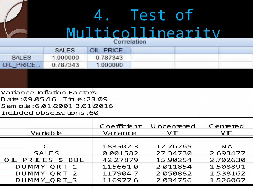
4. Test of Multicollinearity
Variance Inflation FactorsDate: 09/05/16 Time: 23:09Sample: 6/01/2001 3/01/2016Included observations: 60
Coefficient Uncentered CenteredVariable Variance VIF VIF
C 183502.3 12.76765 NASALES 0.001582 27.34730 2.693477
OIL_PRICES_$_BBL_ 42.27879 15.90254 2.702630DUMMY_QRT_1 115661.0 2.011854 1.508891DUMMY_QRT_2 117904.7 2.050882 1.538162DUMMY_QRT_3 116977.6 2.034756 1.526067
Interpretation As we have removed the “Interest Exp.” variable because its
insignificance came up in the first part of our analysis, running Multicollinearity test by including it would be useless.
From, the above analysis we see that there is a 78.73% linear relationship between the two variables, but the Centered VIF of Sales and Oil Prices is 2.693 and 2.702 resp. so we can safely say that the Multicollinearity can be ignored between the two variables. Also, logically we can’t remove either of the variables because both of them are significant in predicting the net profit of the company.
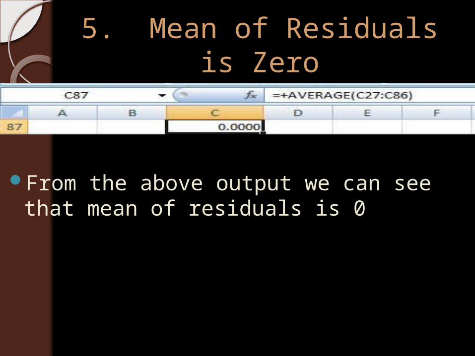
5. Mean of Residuals is Zero
From the above output we can see that mean of residuals is 0
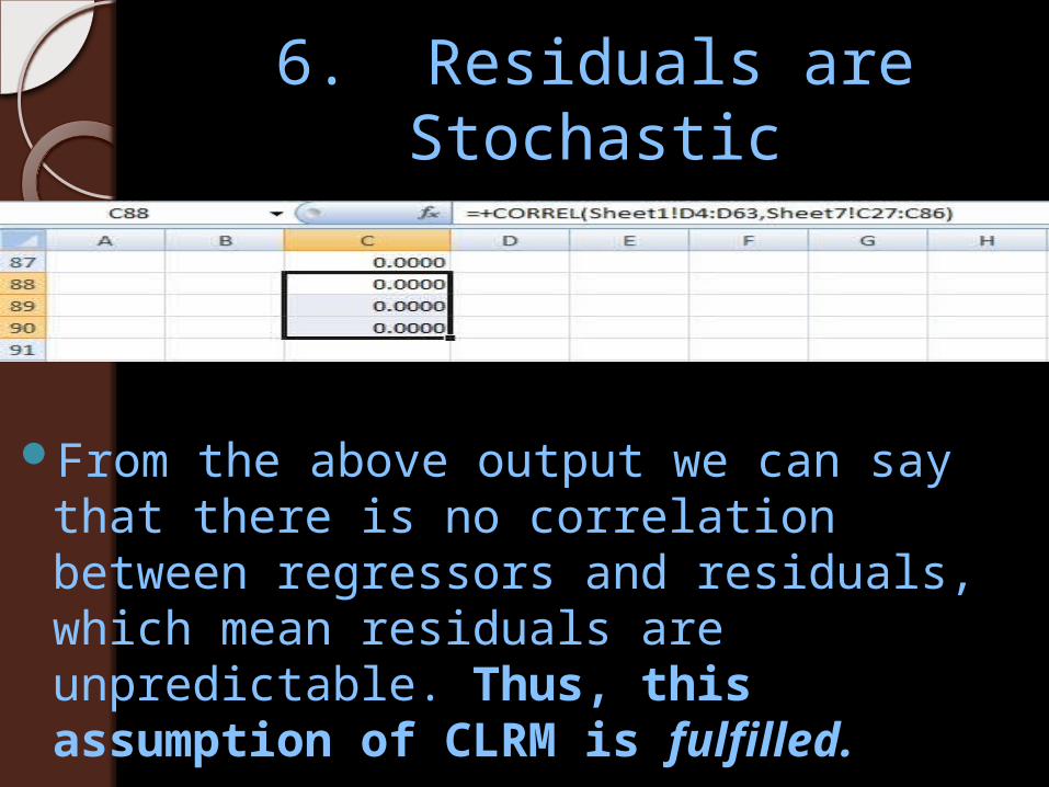
6. Residuals are Stochastic
From the above output we can say that there is no correlation between regressors and residuals, which mean residuals are unpredictable. Thus, this assumption of CLRM is fulfilled.
CONCLUSIONAs, 4 out of 6 assumptions of
CLRM are getting fulfilled, we can say that our model is BLUE i.e.
B: - BestL: - LinearU: - UnbiasedE: - Estimator