Predicting volume of distribution for drug compounds using decision trees

University of Kent

School of Computing

Predicting volume of distribution for drug compounds

using decision trees

NITHYAKALYANI CHINNAIAH

MSc ADVANCED COMPUTER SCIENCE

2015/2016

Under the supervision of Professor Alex Freitas

Word count: About 10,300

ii

Acknowledgements

Firstly, I am grateful to the Almighty for giving me strength, good health and perseverance

to complete this project successfully. My heartfelt thanks to my supervisor, Professor Alex

Freitas for his invaluable guidance and support throughout the project. His timely comments

and suggestions have aided my understanding significantly. I am indebted to my family and

friends. My parents and my sister gave me lots of confidence and encouragement while my

friends stood by me during difficult times. My husband and my daughter put up with me a

lot as I could not spend time with them for the past many months and they have been my

real motivation to complete this project on time.

iii

Abstract

The project is about improving the prediction accuracy of numerical value of volume of

distribution (VD), which is a proportionality constant for drug compounds. While there have

been many approaches using regression with decision trees to predict VD, very few research

studies have been carried out using classification scheme. This project proposes a method

where the two approaches are combined with the addition of a classification confidence

measure. The two stage classification-regression approach is studied with six different data

divisions. In the proposed approach, a test drug’s class is predicted using molecular

structures as attributes and if the prediction confidence is higher than a predetermined

threshold, the log VD value is obtained using regression decision tree built for the particular

class. If the classification prediction is not high, then the approach resorts to standard

regression to obtain log VD value. This two stage approach seems to be promising as the

cross validated performances are improved as compared to standard regression approach for

two of the studied data divisions (one third and one fifth divisions) that gave geometric

mean fold errors (GMFE) of 2.1502 and 2.2013 as compared to the standard regression

GMFE of 2.2373 and 2.2356, respectively.

iv

Table of contents

ABSTRACT

ACKNOWLEDGEMENT

CHAPTER ONE: Introduction

1.1 Contributions

1.2 Structure of dissertation

CHAPTER TWO: Background

2.1 Volume of distribution

2.2 An example of a drug and molecular descriptors

2.3 The classification task of data mining

2.4 Random Forest

2.5 Regression

2.6 Discretisation

CHAPTER THREE: Literature Review on Data Mining for Predicting Volume

of distribution

3.1 Summary of literature review

CHAPTER FOUR: Proposed Methodology

4.1 Discretisation of classes

4.2 Two-stage classification regression approach

4.2.1 Dividing data into training, validation and testing folds

4.2.2 Two stage approach - threshold detection

4.2.3 Error computation

4.3 Fold creation to compare the proposed approach with standard

regression

4.3.1 Standard regression

4.3.2 Proposed two-stage approach

CHAPTER FIVE: Computed Results and Analysis

5.1 Two stage approach

5.1.1 Deciding the threshold for two stage approach

CHAPTER SIX: Conclusion and Future Work Suggestions

6.1 Suggestions for future work

6.2 Reflection

REFERENCES

APPENDIX – Matlab program

ii

iii

1

2

2

3

3

3

4

5

6

6

7

12

13

13

15

15

15

17

18

18

19

20

20

21

26

27

28

29

31

1

Chapter 1: Introduction

The research project is about improving the prediction of volume of distribution (VD) for

drug compounds using classification approaches. VD is one of the most important

pharmacokinetic parameter of drugs, which relates the amount of a drug in the body to the

measured concentration in plasma. VD prediction can be determined using either in-vivo

(animal models, which is time consuming and also raises ethical concerns); in-vitro (which

is also time consuming and requiring costly biological assays) or with a third approach,

known as in-silico. Advantages of theoretical in-silico approaches are high throughput, i.e.

less time consuming computationally and cheaper cost wise (Freitas et al, 2015). So, one can

use this model first and then do in-vivo or in-vitro for more accurate results. Also, only this

approach allows un-synthesised drug to be evaluated and also, reliable in-silico predictions

of the pharmacokinetic parameter would benefit the early stages of drug discovery.

The in-silico predictions are usually performed using regression approaches but very

few researches have been completed using classification approach while several data mining

algorithms have been used to predict VD, the prediction error is still high due to the range of

VD values that is quite large and hence, the hypothesis to be tested here is that the predictive

performance can be improved by discretising the numerical VD values1 into a few categorical

classes and then applying regression. Obviously, the performance will vary depending on the

type of discretisation used.

Hence, the goal of this work would be to predict numerical VD using the predictions

of discretised classes. This dissertation proposes a novel two-stage classification-regression

approach with confidence measure that improves the prediction of VD. The data set that will

be used is extracted from Obach’s database (Obach et al, 2008) and consists of 604 different

drugs (instances).

The motivation behind this work is to predict the VD values for new drugs using data

mining algorithms as mentioned. Extracted knowledge from the research could be used by

pharmaceutical scientists in determining the appropriate dosage regimen. This would benefit

early stages of drug discovery as experimental measurement is not feasible for screening

purposes.

1 Actually, log VD rather than VD due to the large range.

2

1.1 Contributions

The contributions of work here are: • Six different discretisation of log VD values into categorical classes have been

explored;

• Two-stage classification-regression approach developed with random forest (RF)

classification models and RF regression models;

• Classification confidence score, which is measured using the ratio of predictive

accuracy of each class in RF classification in the first stage, and used to decide the

specific RF regression to be used in the second stage;

• Two-stage classification-regression approach using confidence measure that

improves the VD prediction as compared to standard regression.

1.2 Structure of dissertation

The next chapter gives background details of the work such as VD and drug compounds

followed by generic description of classification and regression tasks in data mining. RF,

which is the approach used in this dissertation is also described. A literature review of

relevant work on classification and regression for predicting VD is described in Chapter 3.

Chapter 4 discusses the proposed methodology, which starts with class discretisation and

then the two-stage approach is described. Results and analysis are given in Chapter 5. The

final chapter gives concluding remarks and reflections on the dissertation with some

suggestions for possible future work.

3

Chapter 2: Background

2.1 Volume of distribution

Jambhekar and Breen, 2015 defines VD as proportionality constant and not a physiological

volume. VD relates the plasma concentration with the mass of drug in the body at a time and

is one of the most important pharmacokinetic parameter of drugs. The magnitude of VD is

irrelevant to the actual plasma volume, extracellular or total body volume and could vary

from 7 to 200 litres in a 70 kg subject. Even though VD has no physical meaning, it is

important to decide the correct VD as otherwise it will be difficult to give the appropriate

dosage of drugs to patients. For example, two different drugs could have different VD

because of their physiochemical properties (i.e. chemical structure) and this causes different

concentrations at steady state even if the drugs have the same initial concentrations and

elimination half-lifes. The higher the VD, the higher will be the ability of the drug to be

absorbed by the tissues. Acidic drugs are highly water soluble and do not penetrate into

tissues to a significant degree and hence, have lower VD values. On the other hand, basic

drugs are easily bound to the extracellular tissues and hence have a larger VD. As a result of

this, large range of variation exists for VD which causes the prediction to be a non-trivial

task.

In general, VD prediction can be determined using three approaches, namely in-vivo,

in-vitro and in-silico (Freitas et al, 2015). In-vivo models give a lot of information about the

pharmacokinetics properties of the drugs. But it involves ethical issues as animals are

involved. Furthermore, this approach is time consuming and costly. In-vitro is better than in-

vivo in terms of cost and time but nevertheless, still costly and time consuming as it involves

biological assays. In-silico approaches are based on theoretical models and though these

approaches lack the abundant of information that is possible from the other experimental

approaches, they are less time consuming and less costly. So, it is possible for one to use this

model first and then do in-vivo or in-vitro for more accurate results. In addition, only this

approach allows direct usage of human data which can be used to evaluate the

pharmacokinetics of un-synthesised drug.

2.2 An example of a drug and molecular descriptors

Hydroxychloroquine, which is used to treat malaria is an example of a drug. Its molecular

formula is C18H26ClN3O and has a VD value of 700 L/kg. Figure 1 shows the molecular

structure.

4

Figure 1: Molecular structure for Hydroxychloroquine (image from

https://pubchem.ncbi.nlm.nih.gov/compound/3652#section=2D-Structure)

A drug can be described by a number of molecular descriptors, such as surface

tension, molar volume, the numbers of hydrogen (H) donors and H acceptors, etc. For

instance, for the hydroxychloroquine drug, the number of H donors is 2 and the number of H

acceptors is 4.

2.3 The Classification Task of Data Mining

There are two types of machine learning, in general. The first is supervised learning where

each training example has a pre-defined class label. An example of supervised learning in

data mining is classification task. The second is unsupervised learning where examples are

not assigned pre-defined classes (on purpose or due to being unavailable). An example of

unsupervised learning in data mining is clustering task that is generally useful as a first step

in exploring the data space.

As classification task is used in this project, it is briefly explained in this section.

Classification depends on the predictive characteristics of the features of the data and

usually, has a predefined class or group. The goal of any classification technique is to build a

model using available training data that automatically predicts the class for future unseen

data based on a set of specific characteristics known as features. In other words,

classification would induce data from training set in order to predict the class of test

examples. Examples of classification approaches are Bayesian learning, instance based

learning and decision trees (DT).

Bayesian classification uses Naïve Bayes approach which is based on probability

theory. It assumes each attribute to be independent from each other and hence classification

accuracy is particularly sensitive to redundant attributes. On the other hand, it can handle

missing attributes as attributes are conditionally independent given the class.

5

Decision tree classification builds a DT in a top-down fashion. It selects an attribute

at a time and partitions the examples according to the values of the selected attribute and

repeats this process recursively. Information gain, which is based on information theory is a

commonly used attribute selection criteria. A decision tree can be easily converted into a set

of IF-THEN rules and due to the comprehensibility of the classifier, it is popularly used.

Instance-based learning such as k-nearest neighbour is a straightforward approach

that does not require a model to be built. A new instance is classified as the closest to the

instance in the training data. Some applications may have too complex dataset to allow the

discovery of a simple abstract model and in such cases, this approach is useful.

It is usual to have an ensemble of learning approaches used to increase the class

prediction accuracy where the aggregated output of the classifiers (example majority voting

strategy) would improve predictive accuracy as long as the classifiers are diverse and make

uncorrelated prediction errors. However, the use of such an ensemble requires more

computation.

The performance of classification task is usually evaluated using the predictive

accuracy, which is usually defined as the ratio of correctly classified examples in the test

data over the total number of examples in the test data. Other performance measures are

confusion matrices, sensitivity, precision, recall etc.

It is common to divide the available dataset into training, validation and testing

divisions in order to train and test the developed classifier. Validation data is used to obtain

optimised value of certain parameters used in classifiers. Obviously, how the data is divided

will affect the performance and to minimise this variance in performance resulting from the

data division, cross-validation is typically performed. In a k-fold cross validation, the

available data is divided into k non-overlapping subsets and k-1 folds are used as training

data while the remaining fold used as test data and classification performed. This procedure

is then repeated for k times and the average of the k performances are computed and used as

the actual performance measure. The commonly used k value is 10. In the extreme case, k is

set to the number of examples available and this is known as leave one out approach. The

usefulness of doing k fold cross validation is that it is statistically more reliable than single

training/test set partition but it is disadvantageous as it is computationally expensive.

2.4 Random Forest

Random forest (RF) is defined in Touw et al, 2012 as a versatile classification method that is

appropriate in analysing large data sets. It is a classification technique that builds a model

based on variables to separate the examples into different classes. This algorithm is popular

because of its high prediction accuracy and its ability to provide information about

importance of variables for classification. RF is actually an ensemble of individual decision

6

trees where each tree in the forest is built using a random subset of variables, hence the

name RF.

RF uses, by default (this parameter can be changed), the square root of the total

number of variables as the number of candidate features to be selected at each tree node. The

performance of RF depends on the ability of each individual tree in the forest and the

correlation between them (Breiman, 2001). It works by building an ensemble of trees and

each tree’s prediction is taken as a vote and approaches such as majority voting is to indicate

the most popular class that can significantly improve the overall classification accuracy. To

minimise correlation between the built trees, each tree is built from randomly selected

training examples, as in the bagging method (Breiman, 1996), where each tree is grown

from a sample of training examples randomly selected without replacement from the training

set. Another method is random split selection where, split selection is done randomly at each

node among the k best splits (Dietterich, 1998). Yet, another approach is by selecting the

training set from a random set of weights on the examples in the training set.

RF has a number of advantages. RF uses randomly selected attributes to produce

good results in classification though less so in regression. It is capable of extracting

knowledge from omics data such as when there are interactions between variables (Touw et

al, 2012).

2.5 Regression

Regression is an approach in data mining that predicts the value of a continuous (real-

valued) variable using several independent attributes. Outputs such as age, weight, distance,

temperature, income, sales etc could be predicted using regression techniques. RF decision

trees can be used for regression which would predict numeric quantities rather than

predicting categories. Hence, the same kind of trees can be used but each leaf would contain

a numeric value that is the average of the output values across all the training set examples

that relates to the leaf (Witten et al, 2011).

2.6 Discretisation

The basic idea of discretisation is to convert a continuous (i.e. real-valued) attribute into a

categorical (i.e. discrete or nominal) attribute. There are two approaches that can be

followed in general to do this: class-driven discretisation that chooses interval boundaries

taking into account the class distributions and class-blind discretisation that ignores the

classes of the examples.

7

Chapter 3: Literature Review on Data Mining for Predicting

Volume of Distribution

Many different algorithms like DT based regression, multiple linear regression, neural

networks, have been trained and tested with data sets that contain molecular descriptors of

various compounds along with VD which is determined after intravenous administration of

drugs to healthy people to obtain the prediction accuracy (Jones et al, 2011).

In the study by Freitas et al (2015), Quantitative Structure-Pharmacokinetic

Relationship (QSPKR) model using DTs with feature selection method to predict VD of

chemical compounds (i.e. drugs) was used. This model consists of two phases. In the first

phase, Kt:p (concentration ratio of tissue and plasma) for unknown tissues were predicted

based on molecular descriptors from known Kt:p values of 110 compounds which were

obtained via in vivo or in vitro approaches experimented in animals (i.e. rats). In the second

phase, the above model was used to predict Kt:p using 604 compounds. The predicted Kt:p

values were used along with molecular descriptors to predict VD of compounds.

In the first phase, four types of DTs were used to predict log Kt:p (instead of Kt:p, as

the distribution of VD is skewed): Conventional regression tree, Model tree, If-then

regression rules and Bagging using model tree. The DTs were implemented using M5P

algorithm in WEKA. Mean absolute error (MAE) was calculated using 10 fold cross

validation which showed different models gave the best prediction of log Kt:p for different

types of tissues. Bagging M5P gave lowest error for 7 out of 13 tissues but the authors used

the best method for each tissue.

In the second phase, correlation feature selection (CFS) with genetic search was

used to obtain useful descriptors to predict log VD. This method assigns a higher score to

feature subsets where there is a higher correlation between the subset’s features and the

target variable (indicating the features have good predictive power) and a lower correlation

among the subset’s features (indicating less redundancy among those features). To test the

prediction of VD, the training set consisted of 402 compounds and the test set of 202

compounds. Results obtained using geometric mean fold error (GMFE)2 was used as

performance measure as it is less affected by extreme outliers (as mentioned VD has skewed

distribution). Three different feature set was used:

1. log Kt:p predicted and molecular features (which gave GMFE of 2.61);

2. Only molecular features (which gave GMFE of 2.33);

2 GMFE=antilog10(MAE)

8

3. 56 descriptors selected by CFS (where only two Kt:p for adipose tissue and thymus and

rest 54 from molecular descriptors), which gave a GMFE of 2.29.

Though approach 3 improved GMFE slightly, the improvement was not statistically

significant using t-Test (p=0.577).

The analysis of predicted Kt:p values showed that error comes from large/small VD

values (eg: hydroxychloroquine drug giving VD value of 100 L/kg) and not the Kt:p

prediction. The results were difficult to compare with other studies due to variations in the

data set but GMFE error of 1.56 to 2.78 for inter-species scaling prediction of VD show that

the GMFE error of 2.29 obtained here was acceptable though not the best.

In the study by Amo et al. (2013), anatomical volumes have been used as rough

guidance to classify VD into three classes, namely volume of extracellular fluid class that has

a VD range of 0 – 0.3 L/kg, distribution to the tissues class with VD range of 0.3 – 1 L/kg and

binding to the cellular components class with VD higher than 1 L/kg. The initial dataset

collated by Obach and co-workers (Obach et al 2008) contains 670 compounds with VD and

fu values determined after intravenous administration to healthy people. In this study,

however, the dataset of 642 drugs with VD values ranging from 0.035 – 60 L/kg were used.

Two approaches were used to build predictive models: linear and non-linear models. The

former used Partial Least Square (PLS) with Principal Component Analysis (PCA) and all

descriptors were transformed with unit variance scaling and mean centring before PCA and

PLS analysis. Descriptors with unequal distribution were logarithmically transformed to

obtain better distribution. The second approach which was a non-linear one consisted of non

– linear recursive partitioning classification model that was used to build DTs. To generate

the training set and test set, all compounds were clustered by similarity based on root mean

square deviation. This was done to have compounds from each cluster in both data sets.

Division of training and test set compounds were based on two approaches. One based on VD

and another based on VD and fu (which depends on the binding affinity and capacity of

plasma proteins). The former gives three classes and the later gives six classes (by further

dividing each class as above using VD and with fu either being more than 0.7 or less than

0.7).

Table 1 shows the division of the data set based on VD values. In addition to VD

values, the table also shows a row consisting of log (VD) values as this logarithm

transformation of VD will be utilised in this project to minimise the skewed distribution

caused by some of the high VD values in the dataset. The six class division based on VD and

fu values is not shown here as fu will not be used in this project.

The performance was measured using sensitivity. As an example, Eq. (1) shows the

sensitivity computation for class 1:

9

321

1

FFT

TySensitivit

++

= (1)

where T1 is the number of true positives for class 1, i.e., number of examples in class 1

correctly predicted as class 1, F2 is the number of examples in class 1 wrongly (falsely)

predicted as class 2 and F3 is the number of examples in class 1 wrongly (falsely) predicted

as class 3. The results were high for Class 1 that gave test set sensitivity of 0.71 and for

Class 3 (with test set sensitivity of 0.81) but not so good for Class 2 that only gave test set

sensitivity of 0.32.

Table 1: Division of data set based on VD values by Amo et al, 2013

Class 1 Class 2 Class 3 Total

VD 0 – 0.3 L/kg 0.3 – 1 L/kg ≥ 1 L/kg

log(VD) -1.4559 to -0.5228 -0.5086 to -0.0043 0.0414 to 2.8451

Training 105 96 181 382

Test 62 71 127 260

Total 167 167 308 642

Lombardo et al (2006) utilised a two stage approach to predict the value of VD. In

the first stage, mixture discriminant analysis (MDA) was used to classify into either high or

low class based on VD values: either low VD with VD < 10 L. kg-1

or high VD with VD ≥ 10

L.kg-1

. In the next step, RF regression models trained for each class were used to predict the

VD value. The authors showed that using 31 computed descriptors (examples such as

lipophilicity, ionisation, molecular volume and molecular fragments), the MDA-RF gave a

GMFE of 1.78±11.4. This was much improved as compared to using RF only that gave

GMFE 2.03±15.0. The proposed method also was better than multiple linear regression

approaches using different inputs (31 combined descriptors: GMFE 2.01±11.4; 19

descriptors from simulated annealing: GMFE 2.05±10.1; 16 descriptors based on

physiocochemical intuition: GMFE 2.48±16.2). Furthermore, to show that the MDA-RF will

perform well irrespective of the dataset division, a ten-fold cross validation approach was

used with 384 drugs with each fold either having 38 or 39 compounds, which gave GMFE

ranging from 1.83 to 2.24. Leave one out (LOO) approach was also utilised to study if any

class would be poorly predicted if it had not been included in the model using eight

structural classes with 72 analogues: Steroids (14 compounds), Beta blockers (16

compounds), Fluoroquinolone antibiotics (10 compounds), NSAIDs (7 compounds),

Cephalosporines (17 compounds), Benzodiazepines (15 compounds), Tricyclic

antidepressants (7 compounds) and Morphine-like (10 compounds). This was done as a

10

simulation of real-life prediction when new structural class that has no experimental data

will be tested. The LOO experiment gave GMFE of 1.46 to 2.94 with an average of 1.91.

Berellini et al (2009) also analysed prediction of VD using linear and nonlinear

models using 669 compounds. Four models were used to predict VD: RF, PLS (principal

component (PC) 5), PLS-PC6 and consensus of the two PLS models. GMFE was used to

measure performance. Different number of descriptors was used in each approach. RF model

used 280 molecular descriptors (from MOE and VolSurf+ software) while the PLS models

had 95 and 11 descriptors respectively for PC5 and PC6. Using average of the logarithms of

VD, a consensus model was built using the best models using PLS and RF. Results were

given for nine structural classes with 172 analogues (number of analogues shown in

brackets): Beta adrenergics (27), Benzodiazepines (18), Cephalosporines (27),

Fluoroquinolones (12), Morphinans (12), NSAIDs (16), Nucleosides/nucleotides (31),

Steroids (21) and Tricyclic antidepressants (8) using leave class out (LCO) approach. On

average, consensus model gave GMFE of 1.8 which was also given by PLS-PC5 model. The

other two models both gave GMFE of 2.0. When tested on an external test set of 29

compounds, GMFE from PLS-PC6 model was best with 1.8 while the other models gave

GMFE values from 1.9 to 2.2.

Zhivkova and Doytchinova (2012) looked at VD but only for acidic drugs totalling

132. Genetic algorithm (GA) was used as variable selection procedure from the 178

molecular descriptors available and stepwise linear regression was used to design two

models, once to estimate log VD and another to estimate log (VD/MW). The latter is VD per

unit weight that would eliminate the influence of molecular weight (MW). Descriptors with

non-zero values for less than three molecules were eliminated. The models were assessed by

explained variance (r2) and standard error estimate (SEE). Two cross-validation approaches

were used: leave-one-out cross-validation (LOO-CV) and leave-many-out cross-validation

(LMO-CV using 80%:20% division for training:testing). The best performing descriptors for

log (VD) model selected by GA were xch9, SdsssP_acnt, SssS_acnt, SdssS_acnt, SHsSH,

Hmax, Gmin, and knotpv that gave r2=0.661 and SEE of 0.194. For the second model, the

descriptors were xch7, xch9, SdsssP_acnt, SdssS_acnt, SsSS, Hmax and nelem. This second

model had higher r2 and SEE values of 0.687 and 0.221. External test set (of 30 runs) was

also used to validate the model’s performance using mean fold error (MFE). This external

test was compiled from Berrelini et al (2009) and consisted of 10 acidic drugs. First model

gave MFE of 2.04 while the second one gave MFE of 2.25.

In a recent paper, Zhivkova et al (2015) used 216 basic drugs belonging to different

chemical and therapeutic classes extracted from Obach’s database (Obach et al, 2008). The

dataset was divided into six sets each comprising of 36 drugs each: five for modelling and

one external validation. The five modelling subsets of data were subjected to five-fold cross

11

validation. Logarithm of VD values were used to obtain closer approximation to normal

distribution (i.e. to avoid the skewness in the VD values). Chemical structure of 179

molecular descriptors were computed by ACD/LogD and MDL QSAR software. Models

were validated using randomisation test, leave-one-out cross-validation and leave-group-out

validation using cross-validated coefficient q2, prediction coefficient r

2 for test set, mean

fold error prediction (MFEP) and accuracy. The accuracy (in percentage) was assessed using

predicted and actual VD within two or three fold error. A consensus model using 27 most

frequently emerging descriptors for 180 basic drugs (some drugs were removed as outliers)

gave r2= 0.529 to 0.593 (mean of 0.555), MFEP was 2.24 to 2.38 (mean of 2.31) and

accuracy of 53% for two-fold error (on average). To propose criteria for prediction of VD of

basic drugs, three groups were suggested: small (VD <0.7 L/kg), moderate (0.7 L/kg ≤ VD ≤ 2

L/kg) and large (VD > 2 L/kg). Seven criteria were proposed logP, fB, Dipole, ncirc, Gmin,

SdssC, aaaC_acnt, Cl_acnt, F_acnt: Drugs that meet neither criterion have small VD (<0.7

L/kg), while those meeting three or more criteria have VD > 2L/kg.

Louis and Agrawal (2012) investigated analysis of VD values of anti-infective agents

from J group of the ATC classification. Three approaches namely, multiple linear regression

(MLR), artificial neural network (ANN) and support vector machine (SVM) were used with

theoretical molecular descriptors from 126 drugs (with VD ranging from 0.05 to 33 Lkg-1

).

Initially, compounds were sorted according to the log VD values and every 5th compound was

taken as external test compound. The descriptors were selected using CFS which estimated a

subset of 20 subscriptors from a pool of 1664 descriptors computed using E-DRAGON

software (including 1D, 2D and 3D descriptors). Two performance evaluations method: root

mean square error (RMSE) and MAE were used, which showed that SVM gave the best

performance with RMSE=0.273 and MAE=0.207 on the test dataset. SVM parameter

optimisation was done using 10 fold cross validation.

Demir-Kavuk et al (2011) proposed a framework called DemQSAR combining

feature generation, feature selection, model building and overtraining control to predict VD

and also human clearance (CL). Although Obach’s database (Obach et al, 2008) was used,

only 584 compounds were selected with compounds containing phosphorous, boron, metal

atoms, macrocycles, and fragment-like were removed. This dataset was divided into 338 for

training and remaining approximately 40% (i.e. 246) for testing. Furthermore, 10 fold cross

validation of the whole dataset was also done along with external testing of 29 compounds

used by Berelleni et al (2009). Several software packages were used which gave 404

molecular descriptors for each compound. Combining this with four types of fingerprints

gave a total of 3642 features. Lasso regularization and recursive feature elimination (RFE)

were used as feature selectors. Cross validation performance for VD prediction gave GMFE

12

of 2.01 with all features and with minimal 27 features, GMFE of 2.24 was obtained. With

the same 27 features, external GMFE of 1.81 was obtained.

3.1 Summary of literature review

There are many research studies that have looked into predicting VD using various

algorithms based on regression approaches but only Lombardo et al (2006) has attempted to

implement two stage classification and regression similar to the work proposed here.

Nevertheless, the approach only looked at simple two class division based on VD values on a

smaller subset of 384 drugs in Obach’s database (Obach et al, 2008). Furthermore, the

approach by Lombardo et al did not attempt to measure confidence of classification before

obtaining regressed VD values.

13

Chapter 4 Proposed Methodology

4.1 Discretisation of classes

The proposed methodology consists of two stages where the first stage is classification and

the second stage is regression. In the first stage, VD values are discretised into several

classes and initially, the number of classes to use has to be decided. The simplest approach

would be to divide the data set in certain proportions and there are two ways to do this. One

way is to equally divide the entire data set into certain number of classes such as three

classes – LOW, MEDIUM and HIGH each consisting of 33% of the data. If this is going to

be five classes, then the proportion will be 20% with class set of VERY LOW, LOW,

MEDIUM, HIGH and VERY HIGH. Another way is to divide the data set unequally, for

example dividing some classes with more instances such as in proportions like 20%, 60%,

20% (LOW, MEDIUM, HIGH, respectively) for three classes and for the case of five

classes, it could be such as VERY LOW (10%), LOW (20%), MEDIUM (40%), HIGH

(20%) and VERY HIGH (10%). There are other approaches to divide the data set like using

k-means algorithm, density based algorithm and so on. For the data set utilised in this

research, preliminary analysis showed that some of these methods didn’t work very well.

For example, using k-means for three classes resulted as LOW (90%), MEDIUM (9%),

HIGH (1%) which is not useful as LOW class has very high number of instances and would

skew the classification.

In addition to the proportionality divisions, two more divisions are considered from

literature. One from Lombardo et al (2006) where the entire data set was divided into two

classes with respect to VD values. Instances with VD values <10 L/kg were classified as the

LOW class (consisting of 92%) and the instances with VD values >=10 L/kg were classified

as HIGH class (consisting of 8%). Another is by Amo et al (2013) in which data was divided

into three classes, namely LOW class with log VD values from 0 to 0.3 as LOW (27%), from

0.3 to 1 as MEDIUM (27%) and log VD values higher than 1 as HIGH (46%). Table 1 shows

the class divisions based on VD values for two and three classes while Table 2 shows the

class divisions for five classes. As can be seen from the tables, the division of data is not

exactly in the specified ratio. This is because at the division boundary, there could be several

instances with the same log VD values and as such, these require to be placed in the same

class causing slightly different ratios than the specified ones. For example, 33% division has

201 instances for LOW class, 198 instances for MEDIUM class and 206 instances for HIGH

class. Only 602 drug compounds from Obach’s database are used here as the two extremely

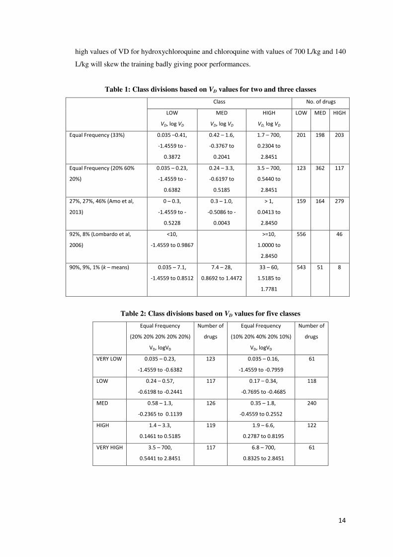
14

high values of VD for hydroxychloroquine and chloroquine with values of 700 L/kg and 140

L/kg will skew the training badly giving poor performances.

Table 1: Class divisions based on VD values for two and three classes

Class No. of drugs

LOW

VD, log VD

MED

VD, log VD

HIGH

VD, log VD

LOW MED HIGH

Equal Frequency (33%) 0.035 –0.41,

-1.4559 to -

0.3872

0.42 – 1.6,

-0.3767 to

0.2041

1.7 – 700,

0.2304 to

2.8451

201 198 203

Equal Frequency (20% 60%

20%)

0.035 – 0.23,

-1.4559 to -

0.6382

0.24 – 3.3,

-0.6197 to

0.5185

3.5 – 700,

0.5440 to

2.8451

123 362 117

27%, 27%, 46% (Amo et al,

2013)

0 – 0.3,

-1.4559 to -

0.5228

0.3 – 1.0,

-0.5086 to -

0.0043

> 1,

0.0413 to

2.8450

159 164 279

92%, 8% (Lombardo et al,

2006)

<10,

-1.4559 to 0.9867

>=10,

1.0000 to

2.8450

556 46

90%, 9%, 1% (k – means) 0.035 – 7.1,

-1.4559 to 0.8512

7.4 – 28,

0.8692 to 1.4472

33 – 60,

1.5185 to

1.7781

543 51 8

Table 2: Class divisions based on VD values for five classes

Equal Frequency

(20% 20% 20% 20% 20%)

VD, logVD

Number of

drugs

Equal Frequency

(10% 20% 40% 20% 10%)

VD, logVD

Number of

drugs

VERY LOW 0.035 – 0.23,

-1.4559 to -0.6382

123 0.035 – 0.16,

-1.4559 to -0.7959

61

LOW 0.24 – 0.57,

-0.6198 to -0.2441

117 0.17 – 0.34,

-0.7695 to -0.4685

118

MED 0.58 – 1.3,

-0.2365 to 0.1139

126 0.35 – 1.8,

-0.4559 to 0.2552

240

HIGH 1.4 – 3.3,

0.1461 to 0.5185

119 1.9 – 6.6,

0.2787 to 0.8195

122

VERY HIGH 3.5 – 700,

0.5441 to 2.8451

117 6.8 – 700,

0.8325 to 2.8451

61

15

4.2 Two-stage Classification Regression approach

4.2.1 Dividing data into training, validation and testing folds

Once the data is discretised into classes, it is further divided into 10 folds with nearly equal

number of instances of each class. Next, with one fold kept as test fold, 9 folds are used with

8 folds for training and the remaining fold for validation. The training data will be used to

build the RF classification and regression trees. The validation data is used to obtain the best

performing threshold to be used with confidence measure that will be explained later. The

data in the test fold is not used here.

4.2.2 Two stage approach - threshold detection

At the start of the two-stage approach, classification DTs are built (with 100 trees and 17

randomly selected variables3 where Matlab’s TreeBagger

4 function is used to build the RF)

using the training data as below:

Bstage1=TreeBagger(trees,dtrain(:,1:293),ctrain,'nvartosample',novar);

where trees is the number of trees in RF (trees=100), novar is the number of variables

(novar=17), ctrain contains the class labels as per the divisions decided earlier. Numeric

values are assigned to each class such as 1 for LOW, 2 for MEDIUM and 3 for HIGH.

Columns 1 to 293 in dtrain contain the 293 attributes of the training data in the fold.

Bstage1 contains the built 100 RF trees.

Next, regression decision trees are built for each class using training data from each

class (again with 100 RF trees and 17 variables). So, in the case of 33%33%33% division,

regression RF is built three times, one for each class as below (example shown for class 1):

regclass1=TreeBagger(trees,train_class1(:,1:293),train_class1(:,294),'Metho

d',...

'regression','nvartosample',novar);

where train_class1 contains training data from class 1 only (with 293 attributes),

train_class1(:,294) contains the log VD values from training data and regclass1

contains the built RF for class 1. Similarly, RF regression tree is built for the rest of the

classes.

Using validation data, the classes of the validation instances are predicted using:

3 17 chosen based on rule of thumb: sqrt (number of attributes).

4 TreeBagger can be run for classification (default) or for regression.

16

[cstage1_val, cScore]=predict(Bstage1,dval(:,1:293));

where Bstage1 contains the built classification RF, dval is the validation data (with

293 attributes), cstage1_val contains the predicted classes and cScore contains the

confidence of prediction for each instance of the validation data. For example, for each

instance in the validation data, the 100 trees could have 20 trees giving prediction as class 1,

50 trees giving prediction as class 2 and 30 trees giving prediction as class 3. This would

give a prediction confidence measure of [0.2 0.5 0.3].

Classification accuracy using the predicted classes of the validation data is found

using cstage1_val with actual labels of the validation data. The overall accuracy is

computed using the number of correctly predicted instances divided by the total number of

instances – this is also done for each class where the number of correctly predicted instances

for the class is divided by the total number of instances for the class. The usefulness of doing

this will become evident later in the discussion.

To decide on the confidence measure i.e., how accurately is the class of that

particular instance is predicted, the following equation is used:

)_(*)_max( confidencetionclassificameanthresholdconfidencetionclassifica > (2)

where threshold varies from 1.1 to 4.0 in steps of 0.1,

mean(classification_confidence) is the mean confidence of the predicted class

outcomes for that instance across all trees in RF and max (classification_confidence)

is the maximum confidence value of these predicted class outcomes. Initially, the threshold

is set at 1.1.

If equation (2) is satisfied for the validation instance as below:

for i=1:length(cScore)

if(max(cScore(:,i))>thres_factor*mean(cScore(:,i)));

predict_ok(i)=1; %which instances are high confidence prediction

end

end

then two stage classification regression approach is used by setting the predict_ok variable

to 1 or else standard regression approach is used (predict_ok =0).

So, for each of the validation instance, if the confidence is exceeded, the respective

regression tree for the predicted class is loaded. For example, for an instance in the

17

validation data with high confidence, if the predicted class is MEDIUM, then the regression

tree built for this MEDIUM class is loaded and the predicted log VD is obtained.

If the confidence is not high (i.e. according to equation (2)), then standard regression

approach is followed by building RF using training data as follows. Standard regression of

log VD values is performed with ensemble of 100 random forest trees built with 17 variables

randomly selected:

Bstdreg=TreeBagger(trees,dtrain(:,1:293),dtrain(:,294),...

'Method','regression','nvartosample',novar);

where trees is the number of trees in RF (trees=100), novar is the number of variables

(novar=17), dtrain columns 1 to 293 contains the 293 attributes of the training data in the

fold and the 294th column in dtrain contains the actual log VD values. Bstdreg contains

the built 100 RF trees.

Hence, the validation instance is subjected to either the two-stage approach or the

standard regression by the following code (example shown for three classes division):

%choose regression model based on predicted class

for i=1:length(cval)

if(str2num(cstage1_val{i})==1 && predict_ok(i)==1) %check predicted

class and high prediction

Vdregnew(i)=predict(regclass1,dval(i,1:293));

elseif(str2num(cstage1_val{i})==2 && predict_ok(i)==1)


elseif(str2num(cstage1_val{i})==3 && predict_ok(i)==1)


else

Vdregnew(i)=predict(Bstdreg,dval(i,1:293)); %use std reg tree if no

high prediction

end

end

The above code loops for all the validation instances where Vdregnew contains the predicted

value of log VD.

4.2.3 Error computation

To obtain the error values of the prediction, RMSE, MAE and GMFE are calculated as

follows:

18

∑=

−=

N

i

DiDi VVN

RMSE1

2')log(log

1

(3)

∑=

−=

N

i

DiDi VVN

MAE1

'|loglog|

1

(4)

MAEGMFE 10= (5)

where log VDi is the actual value given in Obach’s database for the particular validation drug

instance i while log V`Di is the estimated value obtained by either two-stage approach or

standard regression (i.e. Vdregnew above) and N is the number of drug instances in the

validation data.

The above processes 4.2.1 to 4.2.3 is repeated for all the different 90 folds (using

different training and validation data) and average of the errors from 90 folds is computed.

This gives the error for threshold=1.1.

The threshold is now changed to 1.2 (and so on until 4.0 in steps of 0.1) and all the

steps in 4.2.1 to 4.2.3 is repeated for 90 folds and average of the errors from 90 folds is

computed for each threshold. It should be noted that in some cases, the higher threshold

may not have any effect. For example, with three classes, confidence measures with

threshold value about 3.0 will automatically not be confident as the best confidence can

only be 1.0.

The best threshold to use is decided by not only the lowest GMFE error values but

also that there should be at least one confidence prediction in each class. This is to avoid

possible poor performance when using the testing data later.

4.3 Fold creation to compare the proposed approach with standard regression

Once the best threshold has been decided, full data is now divided into 10 folds where 9

folds are used in training and one fold during testing. The folds have nearly equal number of

instances of each class. The data division into folds will be useful to compare the

performance of the proposed approach with standard regression.

4.3.1 Standard regression

Standard regression of log VD values is performed with ensemble of 100 RF trees built with

17 variables randomly selected using training data. This is for comparison with the proposed

two stage approach. The following code is used:

19

Bstdreg=TreeBagger(trees,dtrain(:,1:293),dtrain(:,294),...

'Method','regression','nvartosample',novar);

where dtrain now contains the new training data (9 folds) with 293 attributes and the 294th

column in dtrain contains the actual log VD values. Bstdreg contains the built 100 RF

trees. Testing data (from the remaining fold) are used to obtain the regressed log VD and the

error values computed.

4.3.2 Proposed two-stage approach - testing

Similarly to section 4.2.2, for the two-stage approach, classification RF is built except that

now, the new 9 folds of training data is used and similarly, the regression RF is built for

each class. For each instance in the test data, class prediction and confidence score is

obtained. If the confidence exceeds equation (2) using the threshold decided earlier, then log

VD is predicted using the specific RF regression class. Otherwise, log VD is predicted using

the standard RF regression.

With these predicted log VD values for each test instance, the three errors (RMSE,

MAE, GMFE) are computed. The whole process is then repeated for a different 9 folds of

training and remaining fold for testing and average errors computed for comparison.

All the above steps starting from section 4.1 to 4.3 are carried out for different

discretisation of data and the corresponding results are stored in a text file.

20

Chapter 5 Computed Results and Analysis

In this chapter, the obtained results are given along with analysis of the results.

5.1 Two stage approach

Table 1 shows the classification results for the training and the validation data, i.e. in the

first stage of the two stage approach (without any confidence measure). The class divisions

are VERY LOW, LOW, MEDIUM, HIGH, VERY HIGH represented by classes 1, 2, 3, 4

and 5, respectively and similarly for 3 classes with LOW, MEDIUM, HIGH as 1,2 and 3

respectively. As can be seen for all the data divisions, the overall classification accuracy and

the classification accuracies of the individual classes for the training data are very good

except for the 92%8% division where class 1 has the most number of instances and thus

training is skewed resulting in high accuracy for class 1 and poor for the other class. Some

particular classes (where there are more training instances), the results are 100%, for

example class 3 in 10% 20% 40% 20% 10% data division.

For the validation data, the accuracies are not as good as in the training data and the

higher classification accuracies are for the class instances with more training instances. For

example, for the 20%60%20% division, the validation data accuracies for the classes are

0.3674, 0.8856 and 0.2651.

The poor classification performances for certain classes causes poor prediction

accuracy overall in the test data as well; this obviously will lead to erroneous regression

model loaded in stage two and hence poorer VD prediction. To solve this problem, a suitable

threshold with a confidence measure was explored as explained in the previous chapter.

Table 1: Mean classification accuracy using training and validation data

Training classification accuracy Validation classification accuracy

Overall

accuracy

Class

1

Class

2

Class

3

Class

4

Class

5

Overall

accuracy

Class

1

Class

2

Class

3

Class

4

Class

5

33% 33%

33% 0.9952 0.9984 0.9940 0.9931

0.6676 0.7994 0.5312 0.6721

20% 60%

20% 0.9773 0.9457 1.0000 0.9403

0.6584 0.3674 0.8856 0.2651

20% 20%

20% 20%

20% 0.9974 1.0000 0.9987 0.9993 0.9916 0.9970 0.4642 0.6535 0.2694 0.3932 0.3963 0.6006

10% 20%

40% 20%

10% 0.9821 0.9549 0.9870 1.0000 0.9750 0.9433 0.5215 0.0757 0.4833 0.8269 0.3345 0.2233

92% 8% 0.9429 1.0000 0.2534 0.9251 1.0000 0.0161

27% 27%

46% 0.9778 0.9839 0.9345 0.9998

0.6777 0.6978 0.3301 0.8726

21

5.1.1 Deciding the threshold for two stage approach

Table 2 shows the classification and two stage regression results for validation data from

equally divided three classes (33%33%33%) for varying threshold levels. Results are shown

only up to threshold 2.7 as the results did not change after this threshold. This is because the

threshold will be too high and no data instance will satisfy equation 2 and all the instances

will be processed by standard regression. GMFE of 2.1423 is the lowest error given by

threshold value of 1.5 and this is the threshold used with testing data later.

Table 2: Performance of validation data with varying threshold for 33% 33% 33%

division

Threshold

factor

Validation classification accuracy Two stage regression error

(with confidence measure)

Overall

accuracy

Class1 Class2 Class3 RMSE MAE GMFE

1.1 0.6814 0.8048 0.5385 0.6770 0.5024 0.3537 2.2662

1.2 0.6976 0.8148 0.5450 0.7048 0.4908 0.3466 2.2284

1.3 0.7144 0.8383 0.5498 0.7254 0.4860 0.3429 2.2090

1.4 0.7429 0.8727 0.5404 0.7646 0.4735 0.3360 2.1747

1.5 0.7777 0.9095 0.5364 0.8093 0.4633 0.3295 2.1423

1.6 0.7973 0.9320 0.5046 0.8460 0.4614 0.3302 2.1459

1.7 0.8198 0.9494 0.4867 0.8743 0.4599 0.3320 2.1541

1.8 0.8425 0.9729 0.4672 0.9058 0.4595 0.3347 2.1671

1.9 0.8677 0.9770 0.4557 0.9427 0.4608 0.3384 2.1860

2.0 0.8902 0.9849 0 0.9504 0.4579 0.3378 2.1824

2.1 0.9156 0.9970 0 0.9666 0.4569 0.3387 2.1874

2.2 0.9330 1 0 0.9607 0.4595 0.3414 2.2019

2.3 0.9504 1 0 0 0.4590 0.3429 2.2097

2.4 0.9552 1 0 0 0.4592 0.3433 2.2118

2.5 0.9718 1 0 0 0.4614 0.3453 2.2224

2.6 0.9806 1 0 0 0.4634 0.3477 2.2354

2.7 0 0 0 0 0.4627 0.3468 2.2303

Table 3 shows the classification and two stage regression results for validation data

from unequally divided three classes with more instances for the second class (i.e. 20% 60%

20%) by varying threshold levels. Results are shown only up to threshold 2.7 as the results

did not change after this threshold. This is because the threshold will be too high and no data

instance will satisfy equation 2 and all the instances will be processed by standard

regression. 1.9 is the threshold that gives lowest error with non-zero classification accuracy

for all the individual classes with GMFE of 2.2834.

22

Table 3: Performance of validation data with varying threshold for 20% 60% 20%

division

Threshold

factor



Overall

Accuracy


1.1 0.6593 0.3674 0.8859 0.2651 0.5062 0.3793 2.4027

1.2 0.6576 0.3643 0.8823 0.2612 0.4921 0.3729 2.3714

1.3 0.6620 0.3672 0.8863 0.2635 0.5088 0.3830 2.4249

1.4 0.6764 0.3737 0.8929 0.2806 0.5009 0.3767 2.3878

1.5 0.6873 0.3894 0.9048 0.2472 0.5001 0.3754 2.3809

1.6 0.7128 0.4114 0.9202 0.2318 0.4910 0.3692 2.3482

1.7 0.7364 0.4288 0.9406 0.2275 0.4839 0.3627 2.3118

1.8 0.7622 0.4546 0.9501 0.2136 0.4793 0.3593 2.2944

1.9 0.7879 0.4749 0.9583 0.2003 0.4765 0.3573 2.2834

2.0 0.8057 0.4671 0.9623 0 0.4724 0.3550 2.2704

2.1 0.8329 0 0.9665 0 0.4715 0.3537 2.2632

2.2 0.8477 0 0.9799 0 0.4695 0.3526 2.2577

2.3 0.8804 0 0.9848 0 0.4681 0.3509 2.2485

2.4 0.8879 0 0.9851 0 0.4676 0.3515 2.2516

2.5 0.8892 0 0.9825 0 0.4683 0.3511 2.2489

2.6 0.9151 0 0.9794 0 0.4679 0.3505 2.2458

2.7 0 0 0 0 0.4669 0.3499 2.2428

Table 4: Performance of validation data with varying threshold for

20%20%20%20%20% division

Threshold

factor



Overall

accuracy

Class1 Class2 Class3 Class4 Class5 RMSE MAE GMFE

1.1 0.4652 0.6530 0.2688 0.3936 0.3968 0.6006 0.5384 0.3825 2.4281

1.2 0.4636 0.6461 0.2611 0.3869 0.4194 0.5891 0.5418 0.3855 2.4490

1.3 0.4709 0.6592 0.2708 0.3869 0.4080 0.6059 0.5303 0.3778 2.4036

1.4 0.4751 0.6627 0.2471 0.3982 0.4148 0.6145 0.5288 0.3779 2.4067

1.5 0.4835 0.6835 0.2591 0.4090 0.4126 0.6087 0.5190 0.3742 2.3861

1.6 0.5026 0.7040 0.2550 0.4131 0.4361 0.6398 0.5032 0.3645 2.3317

1.7 0.5279 0.7184 0.2486 0.4542 0.4612 0.6704 0.4905 0.3569 2.2899

1.8 0.5366 0.7296 0.2507 0.4410 0.4437 0.7087 0.4851 0.3536 2.2720

1.9 0.5580 0.7622 0.2630 0.4403 0.4716 0.7256 0.4787 0.3493 2.2487

2.0 0.5623 0.7697 0.2230 0.4674 0.4662 0.7471 0.4744 0.3487 2.2447

2.1 0.5754 0.7944 0.2113 0.4813 0.4704 0.7786 0.4706 0.3469 2.2356

2.2 0.5767 0.8044 0.1678 0 0.4372 0.8023 0.4706 0.3475 2.2388

2.3 0.5832 0.8163 0 0 0.4522 0.8374 0.4690 0.3475 2.2385

2.4 0.6113 0.8402 0 0 0 0 0.4666 0.3464 2.2313

2.5 0.6223 0.8700 0 0 0 0 0.4655 0.3464 2.2315

2.6 0.6388 0.8851 0 0 0 0 0.4642 0.3454 2.2261

2.7 0.6751 0.8978 0 0 0 0 0.4625 0.3444 2.2205

2.8 0.6895 0 0 0 0 0 0.4638 0.3456 2.2269

2.9 0.6966 0 0 0 0 0 0.4636 0.3457 2.2271

3.0 0.7186 0 0 0 0 0 0.4646 0.3466 2.2313

3.1 0.7470 0 0 0 0 0 0.4632 0.3457 2.2253

3.2 0.7587 0 0 0 0 0 0.4638 0.3461 2.2286

3.3 0.7472 0 0 0 0 0 0.4635 0.3469 2.2315

3.4 0 0 0 0 0 0 0.4641 0.3473 2.2331

23

Table 4 shows the classification and two stage regression results for validation data

from equally divided five classes for varying threshold levels. Results are shown only up to

threshold 3.4 as the results did not change after this threshold. Though GMFE of 2.2205 is

the lowest error given by threshold 2.7 but there was not at least one instance in each class

with sufficient high confident prediction. So threshold value of 2.1 which gave GMFE of

2.2356 is used with testing data later.

Table 5: Performance of validation data with varying threshold for

10%20%40%20%10% division

Threshold

factor



Overall

accuracy

Class1 Class2 Class3 Class4 Class5 RMSE MAE GMFE

1.1 0.5153 0.0757 0.4833 0.8269 0.3345 0.1116 0.4942 0.3662 2.3322

1.2 0.5201 0.0791 0.4997 0.8323 0.3517 0.0963 0.4921 0.3639 2.3189

1.3 0.5178 0.0812 0.4981 0.8239 0.3554 0.1054 0.4940 0.3642 2.3208

1.4 0.5139 0.0697 0.4905 0.8241 0.3487 0.0946 0.4948 0.3671 2.3373

1.5 0.5216 0.0716 0.5081 0.8333 0.3541 0.1000 0.4877 0.3611 2.3047

1.6 0.5230 0.0691 0.5117 0.8291 0.3479 0.0947 0.4902 0.3642 2.3196

1.7 0.5307 0.0659 0.5145 0.8318 0.3513 0.0883 0.4863 0.3636 2.3172

1.8 0.5497 0.0631 0.5375 0.8434 0.3588 0.0926 0.4844 0.3611 2.3037

1.9 0.5578 0.0709 0.5442 0.8551 0.3748 0.0867 0.4826 0.3613 2.3041

2.0 0.5663 0.0519 0.5707 0.8512 0.3655 0.0679 0.4821 0.3608 2.3007

2.1 0.5875 0.0504 0.5859 0.8679 0.3825 0.0560 0.4772 0.3575 2.2828

2.2 0.6013 0.0393 0.5978 0.8800 0.3723 0.0575 0.4752 0.3548 2.2682

2.3 0.6189 0 0.6124 0.8910 0.3781 0.0466 0.4729 0.3538 2.2630

2.4 0.6404 0 0.6345 0.9112 0.3912 0 0.4718 0.3520 2.2526

2.5 0.6538 0 0.6572 0.9209 0 0 0.4699 0.3519 2.2526

2.6 0.6647 0 0.6835 0.9274 0 0 0.4676 0.3497 2.2407

2.7 0.6779 0 0.6846 0.9357 0 0 0.4689 0.3509 2.2468

2.8 0.6978 0 0.7128 0.9513 0 0 0.4676 0.3501 2.2424

2.9 0.7110 0 0 0.9589 0 0 0.4665 0.3478 2.2309

3.0 0.7234 0 0 0.9608 0 0 0.4662 0.3483 2.2331

3.1 0.7589 0 0 0.9762 0 0 0.4667 0.3485 2.2339

3.2 0.7545 0 0 0.9713 0 0 0.4672 0.3489 2.2363

3.3 0.7986 0 0 0 0 0 0.4681 0.3497 2.2408

3.4 0.8328 0 0 0.9881 0 0 0.4662 0.3486 2.2349

3.5 0 0 0 0 0 0 0.4670 0.3488 2.2359

Similar to the previous tables, Table 5 shows the results for validation data from

unequally divided five classes with more instances for the third class (i.e. 10% 20% 40%

20% 10%) by varying threshold levels. Results are shown only up to threshold 3.5 as the

results did not change after this threshold. Though GMFE of 2.2309 is the lowest error given

by threshold 2.9 but there was not at least one instance in each class with sufficient high

confident prediction. So threshold value of 2.2 which gives GMFE of 2.2682 is used with

testing data later.

24

Table 6 shows the results for validation data from unequally divided three classes

(27% 27% 46%) for varying threshold levels. Results are shown only up to threshold 2.7 as

the results did not change after this threshold and threshold 1.9 gives the lowest

GMFE=2.2077 and this is used with the testing data.

Table 6: Performance of validation data with varying threshold for 27%27%46%

division

Threshold

factor



Overall

Accuracy


1.1 0.6909 0.7024 0.3326 0.8785 0.5155 0.3786 2.4117

1.2 0.7066 0.7222 0.3401 0.8901 0.5039 0.3721 2.3717

1.3 0.7219 0.7456 0.3187 0.9048 0.4899 0.3654 2.3326

1.4 0.7482 0.7751 0.3228 0.9251 0.4823 0.3593 2.2991

1.5 0.7706 0.8023 0.2868 0.9503 0.4741 0.3538 2.2699

1.6 0.7858 0.8258 0.2692 0.9595 0.4681 0.3485 2.2418

1.7 0.8037 0.8509 0.2431 0.9744 0.4660 0.3465 2.2308

1.8 0.8248 0.8727 0.2332 0.9786 0.4628 0.3437 2.2189

1.9 0.8432 0.9074 0.2155 0.9831 0.4613 0.3417 2.2077

2.0 0.8585 0.9020 0 0.9880 0.4613 0.3429 2.2151

2.1 0.8729 0.9196 0 0.9909 0.4615 0.3439 2.2207

2.2 0.8902 0.9563 0 0.9926 0.4594 0.3429 2.2159

2.3 0.8965 0.9793 0 0.9973 0.4592 0.3441 2.2226

2.4 0.9066 0.9904 0 0.9984 0.4578 0.3429 2.2168

2.5 0.9090 0.9963 0 0 0.4601 0.3454 2.2293

2.6 0.9347 0 0 0 0.4612 0.3465 2.2346

2.7 0 0 0 0 0.4635 0.3492 2.2488

Table 7: Performance of validation data with varying threshold for 92% 8% division

Threshold

factor



Overall

accuracy

Class1 Class2 RMSE MAE GMFE

1.1 0.9044 1 0 0.4911 0.3618 2.3053

1.2 0.9056 1 0 0.4889 0.3610 2.3008

1.3 0.9071 1 0 0.4884 0.3612 2.3016

1.4 0.9100 1 0 0.4858 0.3597 2.2935

1.5 0.9118 1 0 0.4849 0.3591 2.2908

1.6 0.9213 1 0 0.4820 0.3572 2.2808

1.7 0.9353 1 0 0.4770 0.3550 2.2695

1.8 0.9451 1 0 0.4733 0.3542 2.2654

1.9 0.9681 1 0 0.4698 0.3526 2.2570

2.0 0 0 0 0.4677 0.3520 2.2540

Table 7 shows the results from unequally divided two classes with maximum

number of instances for class 1 with 92% 8% division by varying threshold levels. Results

are shown only up to threshold 2.0 as the results did not change after this threshold. Since

25

class 2 errors are 0 for all the cases, this was a special case and threshold value of 1.9 was

used with GMFE error of 2.2570.

Finally, Table 8 shows the standard regression errors for various discretisation using

ten folds of data (9 folds of training and 1 fold of testing), two stage regression errors where

the instances are first classified and then regressed accordingly (without any confidence

measure) and also the two stage regression with confidence measure (i.e. proposed method)

errors. For standard regression, the division of data is irrelevant and hence the performances

just basically depend on the training and testing folds and GMFE errors ranged from 2.2319

to 2.2493, i.e. didn’t change much as expected (slight changes due to RF being used).

Table 8: Standard and two-stage classification regression approach (with and

without) confidence measure using testing data

Data

division

Used

threshold

Standard regression error

Two stage regression

error

(without confidence

measure)

Two stage regression

error

(with confidence

measure)

RMSE MAE GMFE RMSE MAE GMFE RMSE MAE GMFE

33% 33%

33%

1.5 0.4662 0.3485 2.2372 0.5195 0.3659 2.3416 0.4603 0.3306 2.1502

20% 60%

20%

1.9 0.4658 0.3498 2.2425 0.4999 0.3805 2.4139 0.4661 0.3502 2.2440

20% 20%

20% 20%

20%

2.1 0.4635 0.3479 2.2356 0.5266 0.3746 2.3798 0.4597 0.3412 2.2013

10% 20%

40% 20%

10%

2.2 0.4626 0.3476 2.2319 0.4883 0.3598 2.2987 0.4682 0.3481 2.2365

92% 8% 1.9 0.4673 0.3492 2.2493 0.4848 0.3559 2.2914 0.4646 0.3468 2.2373

27% 27%

46%

1.9 0.4645 0.3484 2.2375 0.5260 0.3828 2.4205 0.4672 0.3465 2.2279

The two stage without confidence measure gave GMFE errors from 2.2914 (for

division 92% 8%) to 2.4205 (27% 27% 46%) while using confidence measure improved the

performances for all the divisions when compared to without confidence measure. The best

was given by three equal division (33% 33% 33%) with GMFE error of 2.1502 while the

worse was 20% 60% 20% that gave GMFE error of 2.2440.

When comparing the three methods across the different data divisions, it can be seen

that equal data division (both the three classes and five classes) for the two stage with

confidence measure gave improved performance as compared to standard regression while

92% 8% and 27% 27% 46% divisions gave slightly improved performance and the rest two

(20% 60%20% and 10% 20% 40% 20% 10%) gave slightly poorer results.

26

Chapter 6 Conclusion and Future Work Suggestions

Accurate prediction of volume of distribution using in silico methods is very important

towards estimation of drug delivery and also in the synthesis of new drugs. While in vivo

and in vitro methods exist, these are costly and time consuming. In silico methods also

warrant quick VD predictive results for possible refinement with in vivo and in vitro

approaches.

Most of the studies using in silico approaches use various approaches to predict the

whole range of VD values (usually using Obach et al, 2008 database). However, due to the

large range of VD value (with skewed distribution), the obtained GMFE errors are still

relatively high. In this regard, this MSc dissertation project attempted to refine the prediction

by dividing the instances available in Obach’s database into six different equal and unequal

size divisions, namely 33%33%33%, 20%60%20%, 20%20%20%20%20%,

10%20%40%20%10%,92%8% and 27%27%46%. The aim of the divisions was to reduce

the range of VD values when building a model (in this case, RF decision tree). This would

hopefully increase the accuracy of VD prediction. The step entails a two stage approach,

firstly to build a classification model to predict the class for the test instance and then in the

second stage, to use built regression models for each class to predict the VD value. Decision

tree was the approach suggested by supervisor as it is a popular approach in the literature.

Random Forest (RF) approach was chosen due to its improved ability than a single decision

tree5. The number of attributes available was 293 and the RF approach utilised 17 attributes

chosen randomly from this set of attributes as candidate attributes in each node of a decision

tree.

RF with 100 trees was used, although it is possible to achieve better performance

with higher number of trees, this would cost more computationally. Within the class

divisions, folds of training, validation and testing were created to implement this modified

two stage approach with confidence measure and also to compare the performances with

standard regression using three error measures, RMSE, MAE and GMFE. Initially, the

analysis was done in Weka, but as it was becoming more difficult to handle the data

divisions effectively, Matlab was chosen as the software to perform the analysis.

When the two stage method (classification-regression without confidence measure)

was implemented, it was realised that some classes had poor predictive ability in the first

stage. This was mainly due to unequal class sizes where the class that had more training

5 Supervisor suggested M5P algorithm but I was not able to successfully implement this in Matlab.

27

instances would perform well but the overall accuracy would be poor due to the other

classes performing very poorly. This resulted in higher error values than standard regression

for all the six class divisions. Upon discussing this finding with the supervisor, a modified

two stage approach was suggested. The approach would be different by utilising a

confidence measure of the RF classification in the first stage. While many approaches could

have been explored, due to time limitations, the readily available classification confidence

score as part of the TreeBagger function in Matlab was utilised. The classification

confidence score gave an ability of a measure to decide the effectiveness of the

classification. Using this confidence measure, two stage approach will only be utilised for

the instances where the confidence exceeds a certain threshold and otherwise, the instance

will be subjected to standard regression only.

The best threshold for each division was decided using training and validation folds.

When tested with testing data, the modified approach proved to be useful as it improved the

error measures mainly for the equal class divisions but performing comparably similar to

standard regression in the other class divisions. The best performing division was

33%33%33% that gave Geometric Mean Fold Error (GMFE) of 2.1502 for the two-stage

approach with confidence measure as compared to 2.3416 for the two-stage approach

without confidence measure and 2.2373 for the standard regression approach. For the case of

20%20%20%20%20% data division, the GMFE errors are 2.2013, 2.3798 and 2.2356 for the

proposed two-stage approach with confidence measure, two-stage without confidence

measure and standard regression, respectively.

Exact comparison with the results of others such as Lombardo et al (2006) is not

possible as Lombardo et al. used only 384 drugs that gave GMFE error of 1.83 to 2.24, but

the work here used 602 drugs. Berellini et al, 2009 used 669 compounds and obtained

GMFE of 1.8, but it is not apparent if cross validation of the dataset was implemented.

Freitas et al, 2015 used 402 compounds for training and 202 for testing with 56 attributes

selected with correlation feature selection with genetic search that gave GMFE value of

2.29.

In conclusion, the results obtained here are promising when comparing the current

state of the art and with further work, the prediction of VD values can be made more

accurate.

6.1 Suggestions for future work

Research is of no use if not utilised in some form. In this regard, it is hoped that the outcome

of this research will be extended in future (and perhaps for real-life scenarios) and some

possibilities are:

28

- Explore other class divisions, for example using density based clustering. This could

result in grouping VD values more closely following a certain pattern that could

result in improved prediction accuracy in first stage for the two stage approach.

- Explore other classifiers to use in the first stage, for example deep learning, which is

becoming very popular nowadays and has been shown to give improved

classification results as long as there is sufficient data for training.

- Use other decision tree approaches, both in the first and second stages such as M5P.

Increasing the number of trees could also result in improved performance in both

stages.

- Use feature selection (such as sequential forward floating selection) to select the

appropriate attributes to use, this is likely to give reduced errors if the selected

features have high inter-class variance and low intra-class variance.

- Use of other more advanced confidence measures in the first stage of classification

for example using Bayesian or another probability based approach.

6.2 Reflection

The project was challenging as I did not have any knowledge on pharmacokinetics. I thought

volume of distribution for a drug would be the actual volume of drug delivered! However,

my supervisor assured me that in depth knowledge of pharmacokinetics would not be

required and also provided me with a list of good set of journal papers and a book to read to

equip myself.

Although I had some knowledge acquired on Matlab (through self-study) for one of

my assignments, nevertheless writing codes for a full research problem was daunting. But

breaking up the task into smaller sections as advised by my supervisor proved to be very

useful and small lines of codes were built upon previous codes at a time.

Having a family to manage, time management was probably the most difficult

aspect of my project. However, the pursuit of MSc studies taught me the ability to divide my

time accordingly to strike a balance between the project and family.

My knowledge on machine learning, especially decision trees greatly improved after

implementing the project. I learnt that acquiring knowledge to pass exams is one thing but

practical implementation is yet another matter altogether.

29

References

E. M. del Amo, L. Ghemtio, H. Xhaard, M. Yliperttula, A. Urtti and H. Kidron, “Applying

linear and non-linear methods for parallel prediction of volume of distribution and fraction

of unbound drug,” PLoS One, vol. 8, no. 10, e74758, 2013.

G. Berellini, C. Springer, N. J. Waters and F. Lombardo, “In silico prediction of volume of

distribution in human using linear and nonlinear models on a 669 compound data set,” J.

Med. Chem., vol. 52, pp. 4488–4495, 2009.

L. Breiman, “Bagging predictors,” Machine learning, vol. 24, no. 2, pp. 123-140, 1996.

L. Breiman “Random forests,” Machine learning, vol. 45, no. 1, pp.5-32, 2001.

O. Demir-Kavuk, J. Bentzien, I. Muegge, and E-W. Knapp, “DemQSAR: predicting human

volume of distribution and clearance of drugs,” J. Compu. Aided. Mol. Des., vol. 25, pp.

1121-1133, 2011.

T. G. Dietterich, “Approximate statistical tests for comparing supervised classification

learning algorithms,” Neural Computation, vol. 10, no. 7, pp. 1895-1923, 1998.

A. A. Freitas, K. Limbu, and T. Ghafourian, “Predicting volume of distribution with

decision tree-based regression methods using predicted tissue: plasma partition coefficients,”

J. Cheminformatics, vol. 7, no. 6, 17 pages, 2015.

S. S. Jambhekar, and P. J. Breen, Basic Pharmacokinetics, Second Edition, Pharmaceutical

Press, London, 2012.

R. D. Jones, H. M. Jones, M. Rowland, C. R. Gibson, J. W. T. Yates, J. Y. Chien et. al,

“PhRMA CPCDC initiae on predictive models of human pharmokinetics part 2:

Comparative assessment of prediction methods of volume of distribution,” Journal of

Pharma Science, vol. 100, pp. 4074-4089, 2011.

30

F. Lombardo, R. S. Obach, F. M. DiCapua, G. A. Bakken, J. Lu, D. M. Potter, et al. “A

hybrid mixture discriminant analysis – random forest computational model for the prediction

of volume of distribution of drugs in human,” J. Med. Chem., vol. 49, pp. 2262–2267, 2006.

B. Louis and V. K. Agrawal, “Quantitative structure-pharmacokinetic relationship (QSPkR)

analysis of the volume of distribution values of anti-infective agents from J group of the

ATC classification in humans,” Acta. Pharm., vol. 62, pp. 305–323, 2012.

R. S. Obach, F. Lombardo, and N.J. Waters, “Trend analysis of a database of intravenous

pharmacokinetic parameters in humans for 670 drug compounds,” Drug. Metab. Dispos.,

vol. 36, pp.1385–1405, 2008.

W. G. Touw, J. R. Bayjanov, L. Overmars, L. Backus, J. Boekhorst, M. Wels, and S. A. van

Hijum. “Data mining in the life sciences with random forest: A walk in the park or lost in

the jungle?” Briefings in Bioinformatics, vol. 14, no. 3, pp. 315-326, 2013.

I. H. Witten and E. Frank, Data Mining: Practical Machine Learning Tools and Techniques,

Third Edition, Elsevier/Morgan Kaufman, San Francisco, 2011.

Z. Zhivkova and I. Doytchinova, “Prediction of steady-state volume of distribution of acidic

drugs by quantitative structure-pharmacokinetics relationships,” J. Pharm Sci., vol. 101, pp.

1253–1266, 2012.

Z. Zhivkova, T. Mandova, and I. Doytchinova, “Quantitative structure–pharmacokinetics

relationships analysis of basic drugs: volume of distribution,” Journal of Pharmacy &

Pharmaceutical Sciences, vol. 18, no.3, pp.515-527, 2015.

31

Appendix – Matlab6 program

%program to create ten folds of data for 33%33%33% data division %Nithyakalyani Chinnaiah, [email protected], August 2016

%due to the high number of lines of codes, only codes for one data

%division is being included in Appendix. The full set of codes can

be %found in corpus.

clc; clear all; close all

%just for info, class divisions %y33(1:201)=1; %y33(202:399)=2; %y33(400:602)=3;

x=xlsread('Pharma_data1_only_for_matlab.xlsx'); %read data, 293

%attributes, 1 log Vd temp=randperm(201); %for first class

cls1_fd1=temp(1:20); cls1_fd2=temp(21:40); cls1_fd3=temp(41:60); cls1_fd4=temp(61:80); cls1_fd5=temp(81:100); cls1_fd6=temp(101:120); cls1_fd7=temp(121:140); cls1_fd8=temp(141:160); cls1_fd9=temp(161:180); cls1_fd10=temp(181:201);

ytemp2=202:399; %for second class temp2=ytemp2(randperm(198)); cls2_fd1=temp2(1:20); cls2_fd2=temp2(21:40); cls2_fd3=temp2(41:60); cls2_fd4=temp2(61:80); cls2_fd5=temp2(81:100); cls2_fd6=temp2(101:120); cls2_fd7=temp2(121:140); cls2_fd8=temp2(141:160); cls2_fd9=temp2(161:180); cls2_fd10=temp2(181:198);

ytemp3=400:602; %for third class temp3=ytemp3(randperm(203)); cls3_fd1=temp3(1:20); cls3_fd2=temp3(21:40); cls3_fd3=temp3(41:60); cls3_fd4=temp3(61:80); cls3_fd5=temp3(81:100); cls3_fd6=temp3(101:120); cls3_fd7=temp3(121:140); cls3_fd8=temp3(141:160); cls3_fd9=temp3(161:180); cls3_fd10=temp3(181:203);

6 Mathworks Inc 2016.

32

%splitting the indices for 10 folds of data division with 3 classes fold10=[cls1_fd10,cls2_fd10,cls3_fd10]; fold9=[cls1_fd9,cls2_fd9,cls3_fd9]; fold8=[cls1_fd8,cls2_fd8,cls3_fd8]; fold7=[cls1_fd7,cls2_fd7,cls3_fd7]; fold6=[cls1_fd6,cls2_fd6,cls3_fd6]; fold5=[cls1_fd5,cls2_fd5,cls3_fd5]; fold4=[cls1_fd4,cls2_fd4,cls3_fd4]; fold3=[cls1_fd3,cls2_fd3,cls3_fd3]; fold2=[cls1_fd2,cls2_fd2,cls3_fd2]; fold1=[cls1_fd1,cls2_fd1,cls3_fd1];

%class labels cfold1=[ones(size(cls1_fd1)),1+ones(size(cls2_fd1)),2+ones(size(cls3

_fd1))]; cfold2=[ones(size(cls1_fd2)),1+ones(size(cls2_fd2)),2+ones(size(cls3








_fd9))]; cfold10=[ones(size(cls1_fd10)),1+ones(size(cls2_fd10)),2+ones(size(c

ls3_fd10))];

save datafold33.mat

%%%%%% creating folds for different training, validation and testing

%%%%%%

% fold1 data %%%%%%%%%%%%%%%%%%%% dtrain=[x(fold1,:);x(fold2,:);x(fold3,:);x(fold4,:);x(fold5,:);x(fol

d6,:);x(fold7,:);x(fold8,:)]; %training data dval=x(fold9,:); %validation data

%fold1 labels ctrain=[cfold1,cfold2,cfold3,cfold4,cfold5,cfold6,cfold7,cfold8];

%training data label cval=cfold9; %validation data label

%fold 1 class 1 cls1_train=[cls1_fd1,cls1_fd2,cls1_fd3,cls1_fd4,cls1_fd5,cls1_fd6,cl

s1_fd7,cls1_fd8]; %training data cls1_val= cls1_fd9; %validation fold %fold 1 class 2 cls2_train=[cls2_fd1,cls2_fd2,cls2_fd3,cls2_fd4,cls2_fd5,cls2_fd6,cl

s2_fd7,cls2_fd8]; cls2_val= cls2_fd9; %fold 1 class 3

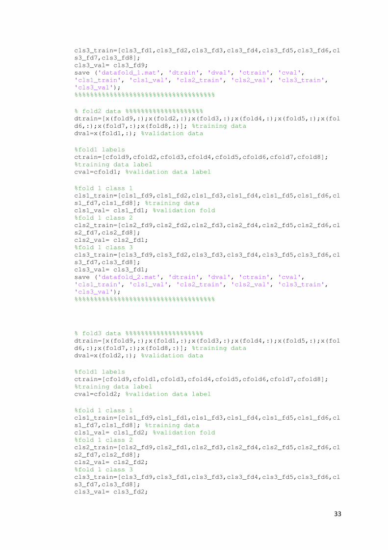
33

cls3_train=[cls3_fd1,cls3_fd2,cls3_fd3,cls3_fd4,cls3_fd5,cls3_fd6,cl

s3_fd7,cls3_fd8]; cls3_val= cls3_fd9; save ('datafold_1.mat', 'dtrain', 'dval', 'ctrain', 'cval',

'cls1_train', 'cls1_val', 'cls2_train', 'cls2_val', 'cls3_train',

'cls3_val'); %%%%%%%%%%%%%%%%%%%%%%%%%%%%%%%%%%%%







s2_fd7,cls2_fd8]; cls2_val= cls2_fd1; %fold 1 class 3 cls3_train=[cls3_fd9,cls3_fd2,cls3_fd3,cls3_fd4,cls3_fd5,cls3_fd6,cl



'cls3_val'); %%%%%%%%%%%%%%%%%%%%%%%%%%%%%%%%%%%%








s3_fd7,cls3_fd8]; cls3_val= cls3_fd2;

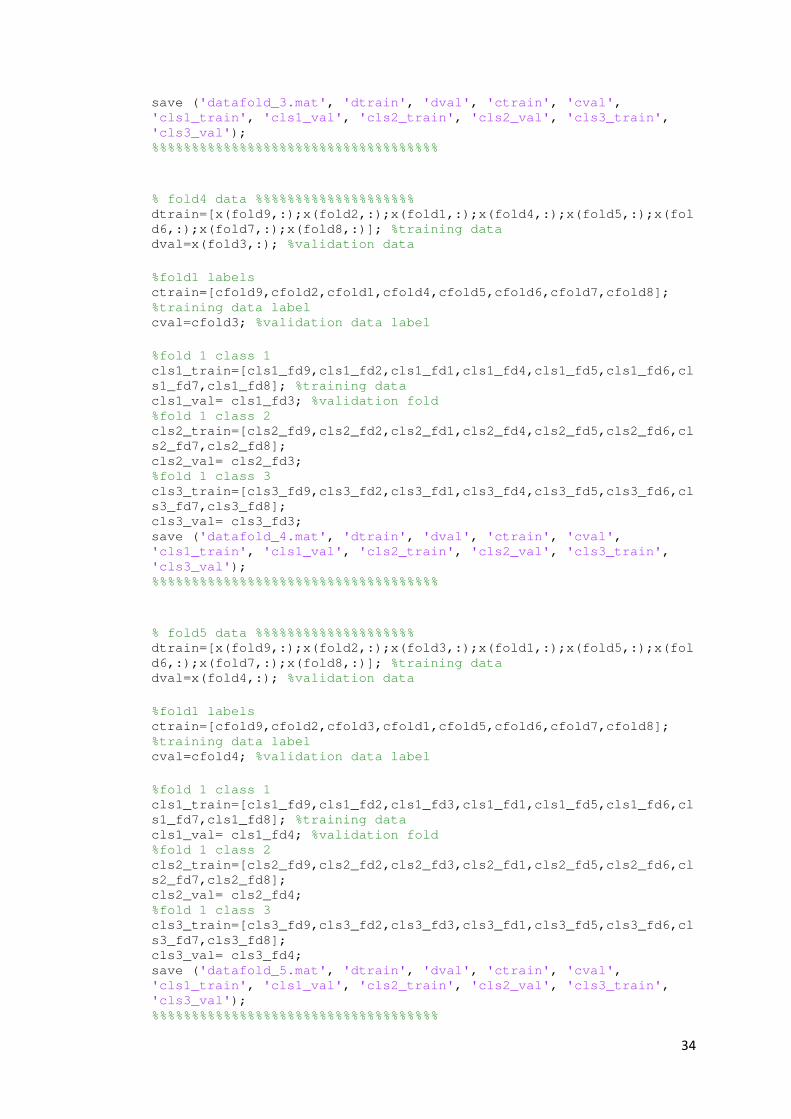
34

save ('datafold_3.mat', 'dtrain', 'dval', 'ctrain', 'cval',


'cls3_val'); %%%%%%%%%%%%%%%%%%%%%%%%%%%%%%%%%%%%










'cls3_val'); %%%%%%%%%%%%%%%%%%%%%%%%%%%%%%%%%%%%










'cls3_val'); %%%%%%%%%%%%%%%%%%%%%%%%%%%%%%%%%%%%

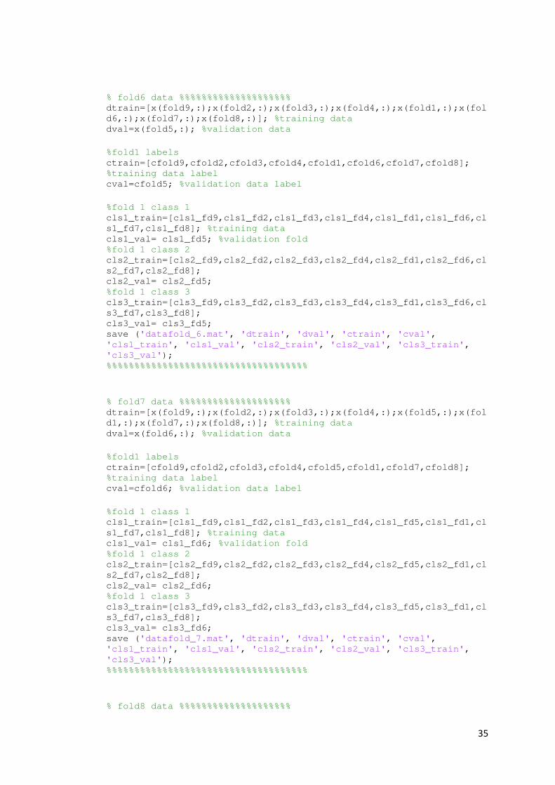
35










'cls3_val'); %%%%%%%%%%%%%%%%%%%%%%%%%%%%%%%%%%%%










'cls3_val'); %%%%%%%%%%%%%%%%%%%%%%%%%%%%%%%%%%%%

% fold8 data %%%%%%%%%%%%%%%%%%%%

36

dtrain=[x(fold9,:);x(fold2,:);x(fold3,:);x(fold4,:);x(fold5,:);x(fol









'cls3_val'); %%%%%%%%%%%%%%%%%%%%%%%%%%%%%%%%%%%%










'cls3_val'); %%%%%%%%%%%%%%%%%%%%%%%%%%%%%%%%%%%%

%%%%%%%%%%%%%%%%%%%%% dtrain=[x(fold1,:);x(fold2,:);x(fold3,:);x(fold4,:);x(fold5,:);x(fol

d6,:);x(fold7,:);x(fold10,:)]; dval=x(fold9,:);

37

ctrain=[cfold1,cfold2,cfold3,cfold4,cfold5,cfold6,cfold7,cfold10]; cval=cfold9; cls1_train=[cls1_fd1,cls1_fd2,cls1_fd3,cls1_fd4,cls1_fd5,cls1_fd6,cl

s1_fd7,cls1_fd10]; cls1_val= cls1_fd9; cls2_train=[cls2_fd1,cls2_fd2,cls2_fd3,cls2_fd4,cls2_fd5,cls2_fd6,cl




'cls3_val'); %%%%%%%%%%%%%%%%%%%%%%%%%%%%%%%%%%%%

% %%%%%%%%%%%%%%%%%%%% dtrain=[x(fold9,:);x(fold2,:);x(fold3,:);x(fold4,:);x(fold5,:);x(fol

d6,:);x(fold7,:);x(fold10,:)]; dval=x(fold1,:); ctrain=[cfold9,cfold2,cfold3,cfold4,cfold5,cfold6,cfold7,cfold10]; cval=cfold1; cls1_train=[cls1_fd9,cls1_fd2,cls1_fd3,cls1_fd4,cls1_fd5,cls1_fd6,cl





'cls3_val'); %%%%%%%%%%%%%%%%%%%%%%%%%%%%%%%%%%%%







'cls3_val'); %%%%%%%%%%%%%%%%%%%%%%%%%%%%%%%%%%%%

%%%%%%%%%%%%%%%%%%%%%

38


d6,:);x(fold7,:);x(fold10,:)]; dval=x(fold3,:); ctrain=[cfold9,cfold2,cfold1,cfold4,cfold5,cfold6,cfold7,cfold10]; cval=cfold3;


s1_fd7,cls1_fd10]; cls1_val= cls1_fd3 cls2_train=[cls2_fd9,cls2_fd2,cls2_fd1,cls2_fd4,cls2_fd5,cls2_fd6,cl




'cls3_val'); %%%%%%%%%%%%%%%%%%%%%%%%%%%%%%%%%%%%

%%%%%%%%%%%%%%%%%%%% dtrain=[x(fold9,:);x(fold2,:);x(fold3,:);x(fold1,:);x(fold5,:);x(fol






'cls3_val'); %%%%%%%%%%%%%%%%%%%%%%%%%%%%%%%%%%%%







'cls3_val');

39

%%%%%%%%%%%%%%%%%%%%%%%%%%%%%%%%%%%%







'cls3_val'); %%%%%%%%%%%%%%%%%%%%%%%%%%%%%%%%%%%%







'cls3_val'); %%%%%%%%%%%%%%%%%%%%%%%%%%%%%%%%%%%%






40



'cls3_val'); %%%%%%%%%%%%%%%%%%%%%%%%%%%%%%%%%%%%







'cls3_val'); %%%%%%%%%%%%%%%%%%%%%%%%%%%%%%%%%%%%







'cls3_val'); %%%%%%%%%%%%%%%%%%%%%%%%%%%%%%%%%%%%





41




'cls3_val'); %%%%%%%%%%%%%%%%%%%%%%%%%%%%%%%%%%%%








'cls3_val'); %%%%%%%%%%%%%%%%%%%%%%%%%%%%%%%%%%%%







'cls3_val'); %%%%%%%%%%%%%%%%%%%%%%%%%%%%%%%%%%%%



s1_fd7,cls1_fd10];

42

cls1_val= cls1_fd5; cls2_train=[cls2_fd8,cls2_fd2,cls2_fd3,cls2_fd4,cls2_fd1,cls2_fd6,cl




'cls3_val'); %%%%%%%%%%%%%%%%%%%%%%%%%%%%%%%%%%%%







'cls3_val'); %%%%%%%%%%%%%%%%%%%%%%%%%%%%%%%%%%%%







'cls3_val'); %%%%%%%%%%%%%%%%%%%%%%%%%%%%%%%%%%%%


d6,:);x(fold7,:);x(fold1,:)]; dval=x(fold10,:); ctrain=[cfold8,cfold2,cfold3,cfold4,cfold5,cfold6,cfold7,cfold1];

43

cval=cfold10; cls1_train=[cls1_fd8,cls1_fd2,cls1_fd3,cls1_fd4,cls1_fd5,cls1_fd6,cl





'cls3_val'); %%%%%%%%%%%%%%%%%%%%%%%%%%%%%%%%%%%%







'cls3_val'); %%%%%%%%%%%%%%%%%%%%%%%%%%%%%%%%%%%%







'cls3_val'); %%%%%%%%%%%%%%%%%%%%%%%%%%%%%%%%%%%%

44







'cls3_val'); %%%%%%%%%%%%%%%%%%%%%%%%%%%%%%%%%%%%








'cls3_val');

%%%%%%%%%%%%%%%%%%%%%%%%%%%%%%%%%%%%






45



'cls3_val'); %%%%%%%%%%%%%%%%%%%%%%%%%%%%%%%%%%%%







'cls3_val'); %%%%%%%%%%%%%%%%%%%%%%%%%%%%%%%%%%%%







'cls3_val'); %%%%%%%%%%%%%%%%%%%%%%%%%%%%%%%%%%%%





46




'cls3_val'); %%%%%%%%%%%%%%%%%%%%%%%%%%%%%%%%%%%%







'cls3_val'); %%%%%%%%%%%%%%%%%%%%%%%%%%%%%%%%%%%%







'cls3_val'); %%%%%%%%%%%%%%%%%%%%%%%%%%%%%%%%%%%%




s2_fd9,cls2_fd10];

47




'cls3_val'); %%%%%%%%%%%%%%%%%%%%%%%%%%%%%%%%%%%%







'cls3_val'); %%%%%%%%%%%%%%%%%%%%%%%%%%%%%%%%%%%%








'cls3_val'); %%%%%%%%%%%%%%%%%%%%%%%%%%%%%%%%%%%%



48






'cls3_val'); %%%%%%%%%%%%%%%%%%%%%%%%%%%%%%%%%%%%







'cls3_val'); %%%%%%%%%%%%%%%%%%%%%%%%%%%%%%%%%%%%







'cls3_val'); %%%%%%%%%%%%%%%%%%%%%%%%%%%%%%%%%%%%


d7,:);x(fold1,:);x(fold10,:)];

49

dval=x(fold9,:); ctrain=[cfold8,cfold2,cfold3,cfold4,cfold5,cfold7,cfold1,cfold10]; cval=cfold9; cls1_train=[cls1_fd8,cls1_fd2,cls1_fd3,cls1_fd4,cls1_fd5,cls1_fd7,cl





'cls3_val'); %%%%%%%%%%%%%%%%%%%%%%%%%%%%%%%%%%%%







'cls3_val'); %%%%%%%%%%%%%%%%%%%%%%%%%%%%%%%%%%%%







'cls3_val'); %%%%%%%%%%%%%%%%%%%%%%%%%%%%%%%%%%%%

% %%%%%%%%%%%%%%%%%%%%

50







'cls3_val'); %%%%%%%%%%%%%%%%%%%%%%%%%%%%%%%%%%%%







'cls3_val'); %%%%%%%%%%%%%%%%%%%%%%%%%%%%%%%%%%%%







51



'cls3_val'); %%%%%%%%%%%%%%%%%%%%%%%%%%%%%%%%%%%%







'cls3_val'); %%%%%%%%%%%%%%%%%%%%%%%%%%%%%%%%%%%%







'cls3_val'); %%%%%%%%%%%%%%%%%%%%%%%%%%%%%%%%%%%%




52





'cls3_val'); %%%%%%%%%%%%%%%%%%%%%%%%%%%%%%%%%%%%







'cls3_val'); %%%%%%%%%%%%%%%%%%%%%%%%%%%%%%%%%%%%







'cls3_val'); %%%%%%%%%%%%%%%%%%%%%%%%%%%%%%%%%%%%



53






'cls3_val'); %%%%%%%%%%%%%%%%%%%%%%%%%%%%%%%%%%%%







'cls3_val'); %%%%%%%%%%%%%%%%%%%%%%%%%%%%%%%%%%%%







'cls3_val'); %%%%%%%%%%%%%%%%%%%%%%%%%%%%%%%%%%%%


d7,:);x(fold9,:);x(fold10,:)];

54

dval=x(fold3,:); ctrain=[cfold8,cfold2,cfold1,cfold5,cfold6,cfold7,cfold9,cfold10]; cval=cfold3;






'cls3_val'); %%%%%%%%%%%%%%%%%%%%%%%%%%%%%%%%%%%%







'cls3_val'); %%%%%%%%%%%%%%%%%%%%%%%%%%%%%%%%%%%%







'cls3_val'); %%%%%%%%%%%%%%%%%%%%%%%%%%%%%%%%%%%%

55







'cls3_val'); %%%%%%%%%%%%%%%%%%%%%%%%%%%%%%%%%%%%







'cls3_val'); %%%%%%%%%%%%%%%%%%%%%%%%%%%%%%%%%%%%






56



'cls3_val'); %%%%%%%%%%%%%%%%%%%%%%%%%%%%%%%%%%%%







'cls3_val'); %%%%%%%%%%%%%%%%%%%%%%%%%%%%%%%%%%%%







'cls3_val'); %%%%%%%%%%%%%%%%%%%%%%%%%%%%%%%%%%%%





57




'cls3_val'); %%%%%%%%%%%%%%%%%%%%%%%%%%%%%%%%%%%%








'cls3_val'); %%%%%%%%%%%%%%%%%%%%%%%%%%%%%%%%%%%%







'cls3_val'); %%%%%%%%%%%%%%%%%%%%%%%%%%%%%%%%%%%%



s1_fd9,cls1_fd10];

58





'cls3_val'); %%%%%%%%%%%%%%%%%%%%%%%%%%%%%%%%%%%%







'cls3_val'); %%%%%%%%%%%%%%%%%%%%%%%%%%%%%%%%%%%%







'cls3_val'); %%%%%%%%%%%%%%%%%%%%%%%%%%%%%%%%%%%%


d7,:);x(fold9,:);x(fold1,:)]; dval=x(fold10,:); ctrain=[cfold8,cfold2,cfold4,cfold5,cfold6,cfold7,cfold9,cfold1];

59

cval=cfold10; cls1_train=[cls1_fd8,cls1_fd2,cls1_fd4,cls1_fd5,cls1_fd6,cls1_fd7,cl





'cls3_val'); %%%%%%%%%%%%%%%%%%%%%%%%%%%%%%%%%%%%







'cls3_val'); %%%%%%%%%%%%%%%%%%%%%%%%%%%%%%%%%%%%







'cls3_val'); %%%%%%%%%%%%%%%%%%%%%%%%%%%%%%%%%%%%

% %%%%%%%%%%%%%%%%%%%%

60







'cls3_val'); %%%%%%%%%%%%%%%%%%%%%%%%%%%%%%%%%%%%








'cls3_val'); %%%%%%%%%%%%%%%%%%%%%%%%%%%%%%%%%%%%







'cls3_val');

61

%%%%%%%%%%%%%%%%%%%%%%%%%%%%%%%%%%%%







'cls3_val'); %%%%%%%%%%%%%%%%%%%%%%%%%%%%%%%%%%%%







'cls3_val'); %%%%%%%%%%%%%%%%%%%%%%%%%%%%%%%%%%%%






62



'cls3_val'); %%%%%%%%%%%%%%%%%%%%%%%%%%%%%%%%%%%%







'cls3_val'); %%%%%%%%%%%%%%%%%%%%%%%%%%%%%%%%%%%%







'cls3_val'); %%%%%%%%%%%%%%%%%%%%%%%%%%%%%%%%%%%%






63



'cls3_val'); %%%%%%%%%%%%%%%%%%%%%%%%%%%%%%%%%%%%







'cls3_val'); %%%%%%%%%%%%%%%%%%%%%%%%%%%%%%%%%%%%








'cls3_val'); %%%%%%%%%%%%%%%%%%%%%%%%%%%%%%%%%%%%




64





'cls3_val'); %%%%%%%%%%%%%%%%%%%%%%%%%%%%%%%%%%%%







'cls3_val'); %%%%%%%%%%%%%%%%%%%%%%%%%%%%%%%%%%%%







'cls3_val'); %%%%%%%%%%%%%%%%%%%%%%%%%%%%%%%%%%%%



65






'cls3_val'); %%%%%%%%%%%%%%%%%%%%%%%%%%%%%%%%%%%%







'cls3_val'); %%%%%%%%%%%%%%%%%%%%%%%%%%%%%%%%%%%%

66

%program to compute threshold for the two stage approach using

%training and validation folds

clc; close all; clear all;

trees = 100; novar = 17; %decision tree parameters load datafold33.mat %load the general 10 fold divisions fid=fopen('fold33n.txt','w'); %file to write results

flagg=1;

for thres=1:30 %for varying confidence levels disp(thres) clearvars -except flagg thres fid trees novar x Bstdreg Bstage1

regclass1 regclass2 regclass3;

thres_factor = 1+0.1*thres; %for confidence measure

RMSEstdreg=0; MAEstdreg=0; GMFEstdreg=0; Accu_train_all=0;

Accu_train_cls1=0; Accu_train_cls2=0; Accu_train_cls3=0; Accu_val_all=0; Accu_val_cls1=0; Accu_val_cls2=0; Accu_val_cls3=0;

RMSE_class1=0; MAE_class1=0; GMFE_class1=0; RMSE_class2=0;

MAE_class2=0; GMFE_class2=0; RMSE_class3=0; MAE_class3=0;

GMFE_class3=0; RMSEreg=0; MAEreg=0; GMFEreg=0; Accu_p=0; Accu_p1=0; Accu_p2=0;

Accu_p3=0;

RMSEregnew=0; MAEregnew=0; GMFEregnew=0; pok=0; pct=0;

for fold=1:90

clear Vdfinal Vdregnew Vdreg dtrain dtest dval ctrain cval ctest

cls1_train cls1_val cls2_train cls2_val cls3_train cls3_val;

if (fold==1) load datafold_1.mat end if (fold==2) load datafold_2.mat end if (fold==3) load datafold_3.mat end if (fold==4) load datafold_4.mat end if (fold==5) load datafold_5.mat end if (fold==6) load datafold_6.mat end if (fold==7) load datafold_7.mat end if (fold==8) load datafold_8.mat end

67

if (fold==9) load datafold_9.mat end if (fold==10) load datafold_10.mat end if (fold==11) load datafold_11.mat end if (fold==12) load datafold_12.mat end if (fold==13) load datafold_13.mat end if (fold==14) load datafold_14.mat end if (fold==15) load datafold_15.mat end if (fold==16) load datafold_16.mat end if (fold==17) load datafold_17.mat end if (fold==18) load datafold_18.mat end if (fold==19) load datafold_19.mat end if (fold==20) load datafold_20.mat end if (fold==21) load datafold_21.mat end if (fold==22) load datafold_22.mat end if (fold==23) load datafold_23.mat end if (fold==24) load datafold_24.mat end if (fold==25) load datafold_25.mat end if (fold==26) load datafold_26.mat end if (fold==27) load datafold_27.mat end if (fold==28) load datafold_28.mat end if (fold==29)

68

load datafold_29.mat end if (fold==30) load datafold_30.mat end if (fold==31) load datafold_31.mat end if (fold==32) load datafold_32.mat end if (fold==33) load datafold_33.mat end if (fold==34) load datafold_34.mat end if (fold==35) load datafold_35.mat end if (fold==36) load datafold_36.mat end if (fold==37) load datafold_37.mat end if (fold==38) load datafold_38.mat end if (fold==39) load datafold_39.mat end if (fold==40) load datafold_40.mat end if (fold==41) load datafold_41.mat end if (fold==42) load datafold_42.mat end if (fold==43) load datafold_43.mat end if (fold==44) load datafold_44.mat end if (fold==45) load datafold_45.mat end if (fold==46) load datafold_46.mat end if (fold==47) load datafold_47.mat end if (fold==48) load datafold_48.mat end if (fold==49) load datafold_49.mat

69

end if (fold==50) load datafold_50.mat end if (fold==51) load datafold_51.mat end if (fold==52) load datafold_52.mat end if (fold==53) load datafold_53.mat end if (fold==54) load datafold_54.mat end if (fold==55) load datafold_55.mat end if (fold==56) load datafold_56.mat end if (fold==57) load datafold_57.mat end if (fold==58) load datafold_58.mat end if (fold==59) load datafold_59.mat end if (fold==60) load datafold_60.mat end if (fold==61) load datafold_61.mat end if (fold==62) load datafold_62.mat end if (fold==63) load datafold_63.mat end if (fold==64) load datafold_64.mat end if (fold==65) load datafold_65.mat end if (fold==66) load datafold_66.mat end if (fold==67) load datafold_67.mat end if (fold==68) load datafold_68.mat end if (fold==69) load datafold_69.mat end

70

if (fold==70) load datafold_70.mat end if (fold==71) load datafold_71.mat end if (fold==72) load datafold_72.mat end if (fold==73) load datafold_73.mat end if (fold==74) load datafold_74.mat end if (fold==75) load datafold_75.mat end if (fold==76) load datafold_76.mat end if (fold==77) load datafold_77.mat end if (fold==78) load datafold_78.mat end if (fold==79) load datafold_79.mat end if (fold==80) load datafold_80.mat end if (fold==81) load datafold_81.mat end if (fold==82) load datafold_82.mat end if (fold==83) load datafold_83.mat end if (fold==84) load datafold_84.mat end if (fold==85) load datafold_85.mat end if (fold==86) load datafold_86.mat end if (fold==87) load datafold_87.mat end if (fold==88) load datafold_88.mat end if (fold==89) load datafold_89.mat end if (fold==90)

71

load datafold_90.mat end

%if (flagg==1)

%%%%%%%%%%%% standard regression %%%%%%%%%%%%%%%%%%% Bstdreg=TreeBagger(trees,dtrain(:,1:293),dtrain(:,294),'Method','reg

ression','nvartosample',novar); Vdstdreg=predict(Bstdreg,dval(:,1:293)); RMSEstdreg=sqrt(mean((Vdstdreg-dval(:,294)).^2))+RMSEstdreg; MAEstdreg=mean(abs(Vdstdreg-dval(:,294)))+MAEstdreg; GMFEstdreg=(10^(mean(abs(Vdstdreg-dval(:,294)))))+GMFEstdreg; %%%%%%%%%%%%%%%%%%%%%%%%%%%%%%%%%%%%%%%%%%%%%%%%%%%%

%%%%%%%%%%%%%%%%% random forest decision trees

%%%%%%%%%%%%%%%%%%%%%% %all rows of training data & all attributes except log Vd Bstage1=TreeBagger(trees,dtrain(:,1:293),ctrain,'nvartosample',novar

);

%Random forest classification; predicting class using training data cstage1_train=predict(Bstage1,dtrain(:,1:293)); cnt1=0;cnt2=0;cnt3=0; %initialisation of array to store correct

prediction for i=1:length(ctrain) if((str2num(cstage1_train{i}))==ctrain(i) && ctrain(i)==1)

%checking if class prediction matches cnt1=cnt1+1; end if((str2num(cstage1_train{i}))==ctrain(i) && ctrain(i)==2)

%class2 cnt2=cnt2+1; end if((str2num(cstage1_train{i}))==ctrain(i) && ctrain(i)==3)

%class3 cnt3=cnt3+1; end end

Accu_train_all=(cnt1+cnt2+cnt3)/length(ctrain)+Accu_train_all;

%total train accuracy Accu_train_cls1=cnt1/sum(ctrain==1)+Accu_train_cls1; Accu_train_cls2=cnt2/sum(ctrain==2)+Accu_train_cls2; Accu_train_cls3=cnt3/sum(ctrain==3)+Accu_train_cls3;

%predictiong class using validation data [cstage1_val, cScore]=predict(Bstage1,dval(:,1:293)); %cScore gives

confidence of prediction

cnt1=0;cnt2=0;cnt3=0; %initialisation of array to store correct

prediction for i=1:length(cval) if((str2num(cstage1_val{i}))==cval(i) && cval(i)==1) %checking

if class prediction matches cnt1=cnt1+1; end if((str2num(cstage1_val{i}))==cval(i) && cval(i)==2) %class2 cnt2=cnt2+1; end if((str2num(cstage1_val{i}))==cval(i) && cval(i)==3) %class3

72

cnt3=cnt3+1; end end

Accu_val_all=(cnt1+cnt2+cnt3)/length(cval)+Accu_val_all; %total

validation accuracy Accu_val_cls1=cnt1/sum(cval==1)+Accu_val_cls1; Accu_val_cls2=cnt2/sum(cval==2)+Accu_val_cls2; Accu_val_cls3=cnt3/sum(cval==3)+Accu_val_cls3;

%%%%%%%%%%%%%%% build regression trees for three classes

%%%%%%%%%%%%%%%%%%%%%%%%%%%%

%for class1 train_class1=x(cls1_train,:); %8 fold train data val_class1=x(cls1_val,:); %validation data

%regression with random forest regclass1=TreeBagger(trees,train_class1(:,1:293),train_class1(:,294)

,'Method','regression','nvartosample',novar); fitclass1=predict(regclass1,val_class1(:,1:293)); %predicted logVd RMSE_class1=sqrt(mean((fitclass1-

val_class1(:,294)).^2))+RMSE_class1; %root mean square error MAE_class1=mean(abs(fitclass1-val_class1(:,294)))+MAE_class1; %mean

absolute error GMFE_class1=(10^(mean(abs(fitclass1-

val_class1(:,294)))))+GMFE_class1; %GMFE error

%for class2 train_class2=x(cls2_train,:); val_class2=x(cls2_val,:); regclass2=TreeBagger(trees,train_class2(:,1:293),train_class2(:,294)

,'Method','regression','nvartosample',novar); fitclass2=predict(regclass2,val_class2(:,1:293)); RMSE_class2=sqrt(mean((fitclass2-

val_class2(:,294)).^2))+RMSE_class2; MAE_class2=mean(abs(fitclass2-val_class2(:,294)))+MAE_class2; GMFE_class2=(10^(mean(abs(fitclass2-

val_class2(:,294)))))+GMFE_class2;

%for class3 train_class3=x(cls3_train,:); val_class3=x(cls3_val,:); regclass3=TreeBagger(trees,train_class3(:,1:293),train_class3(:,294)

,'Method','regression','nvartosample',novar); fitclass3=predict(regclass3,val_class3(:,1:293)); RMSE_class3=sqrt(mean((fitclass3-

val_class3(:,294)).^2))+RMSE_class3; MAE_class3=mean(abs(fitclass3-val_class3(:,294)))+MAE_class3; GMFE_class3=(10^(mean(abs(fitclass3-

val_class3(:,294)))))+GMFE_class3;

%choose regression model based on predicted class for i=1:length(cval) if(str2num(cstage1_val{i})==1)

73

Vdreg(i)=predict(regclass1,dval(i,1:293)); elseif(str2num(cstage1_val{i})==2) Vdreg(i)=predict(regclass2,dval(i,1:293)); elseif(str2num(cstage1_val{i})==3) Vdreg(i)=predict(regclass3,dval(i,1:293)); end end Vdreg=Vdreg';

RMSEreg=sqrt(mean((Vdreg-dval(:,294)).^2))+RMSEreg; MAEreg=mean(abs(Vdreg-dval(:,294)))+MAEreg; GMFEreg=(10^(mean(abs(Vdreg-dval(:,294)))))+GMFEreg;

%end %flagg loop

%%%%% to find the appropriate threshold for confidence %%%%%%%%%%%%%

[cstage1_val, cScore]=predict(Bstage1,dval(:,1:293)); %cScore gives

confidence of prediction cScore=cScore';

predict_ok(1:length(cScore))=0; for i=1:length(cScore) if(max(cScore(:,i))>thres_factor*mean(cScore(:,i))); predict_ok(i)=1; %which instances are high confidence prediction end end pok=sum(predict_ok)+pok; %just to keep track

%Storing high confidence and correct prediction p_cnt(1:length(cval))=0; for i=1:length(cval) if((str2num(cstage1_val{i}))==cval(i) && predict_ok(i)==1)

%checking if class prediction matches and high confidence p_cnt(i)=1; %high confidence and correct prediction end end pct=sum(p_cnt)+pct; %just to keep track

%just finding accuracy of (high prediction and high confidence)/high

confidence Accu_p=sum(p_cnt)/sum(predict_ok)+Accu_p; nv1=length(cls1_val); nv2=length(cls2_val); nv3=length(cls3_val); Accu_p1=sum(p_cnt(1:nv1))/sum(predict_ok(1:nv1))+Accu_p1; %class 1

accuracy Accu_p2=sum(p_cnt(nv1+1:nv1+nv2))/sum(predict_ok(nv1+1:nv1+nv2))+Acc

u_p2; %class 2 Accu_p3=sum(p_cnt(nv1+nv2+1:nv1+nv2+nv3))/sum(predict_ok(nv1+nv2+1:n

v1+nv2+nv3))+Accu_p3; %class 3

%choose regression model based on predicted class for i=1:length(cval) if(str2num(cstage1_val{i})==1 && predict_ok(i)==1) %check

predicted class and high prediction Vdregnew(i)=predict(regclass1,dval(i,1:293)); elseif(str2num(cstage1_val{i})==2 && predict_ok(i)==1) Vdregnew(i)=predict(regclass2,dval(i,1:293)); elseif(str2num(cstage1_val{i})==3 && predict_ok(i)==1)

74

Vdregnew(i)=predict(regclass3,dval(i,1:293)); else Vdregnew(i)=predict(Bstdreg,dval(i,1:293)); %use std reg tree if

no high prediction end end Vdregnew=Vdregnew';

RMSEregnew=sqrt(mean((Vdregnew-dval(:,294)).^2))+RMSEregnew; %root

mean square error MAEregnew=mean(abs(Vdregnew-dval(:,294)))+MAEregnew; %mean absolute

error GMFEregnew=(10^(mean(abs(Vdregnew-dval(:,294)))))+GMFEregnew;

end %fold loop

if (flagg==1) fprintf(fid,'\nRegression (standard) errors

(RMSEstdreg,MAEstdreg,GMFEstdreg):\t%f\t%f\t%f\n',RMSEstdreg/90,MAEs

tdreg/90,GMFEstdreg/90); fprintf(fid,'Training classification accuracy (Accu_train_all,

Accu_train_cls1, Accu_train_cls2,

Accu_train_cls3):\t%f\t%f\t%f\t%f\n',Accu_train_all/90,

Accu_train_cls1/90, Accu_train_cls2/90, Accu_train_cls3/90); fprintf(fid,'Validation classification accuracy (Accu_val_all,

Accu_val_cls1, Accu_val_cls2,

Accu_val_cls3):\t%f\t%f\t%f\t%f\n',Accu_val_all/90,

Accu_val_cls1/90, Accu_val_cls2/90, Accu_val_cls3/90); fprintf(fid,'Validation regression accuracy (class 1, RMSE1, MAE1,

GMFE1):\t%f\t%f\t%f\n',RMSE_class1/90, MAE_class1/90,

GMFE_class1/90); fprintf(fid,'Validation regression accuracy (class 2, RMSE2, MAE2,


GMFE_class2/90); fprintf(fid,'Validation regression accuracy (class 3, RMSE3, MAE3,


GMFE_class3/90); fprintf(fid,'Regression errors 2 stage, no

thres(RMSEreg,MAEreg,GMFEreg):\t%f\t%f\t%f\n',RMSEreg/9,MAEreg/90,GM

FEreg/90);

flagg=0; end

fprintf(fid,'Thres_factor:\t%f\n',thres_factor); fprintf(fid,'Testing classification accuracy with high

confidence(Accu_p, Accu_p1, Accu_p2,

Accu_p3)):\t%f\t%f\t%f\t%f\n',Accu_p/90, Accu_p1/90, Accu_p2/90,

Accu_p3/90); fprintf(fid,'Regression errors 2 stage with thres

(RMSEregnew,MAEregnew,GMFEregnew,predict_ok,p_cnt):\t%f\t%f\t%f\t%d\

t%d\n',RMSEregnew/90,MAEregnew/90,GMFEregnew/90,pok/90,pct/90);

end %threshold loop

fclose(fid);

75

%program to create ten folds of data for 33%33%33% data division %Nithyakalyani Chinnaiah, [email protected], August 2016

clc; clear all; close all

%just for info, class divisions %y33(1:201)=1; %y33(202:399)=2; %y33(400:602)=3;

x=xlsread('Pharma_data1_only_for_matlab.xlsx'); %read data, 293

attributes, 1 log Vd temp=randperm(201); %for first class

cls1_fd1=temp(1:20); cls1_fd2=temp(21:40); cls1_fd3=temp(41:60); cls1_fd4=temp(61:80); cls1_fd5=temp(81:100); cls1_fd6=temp(101:120); cls1_fd7=temp(121:140); cls1_fd8=temp(141:160); cls1_fd9=temp(161:180); cls1_fd10=temp(181:201);

ytemp2=202:399; %for second class temp2=ytemp2(randperm(198)); cls2_fd1=temp2(1:20); cls2_fd2=temp2(21:40); cls2_fd3=temp2(41:60); cls2_fd4=temp2(61:80); cls2_fd5=temp2(81:100); cls2_fd6=temp2(101:120); cls2_fd7=temp2(121:140); cls2_fd8=temp2(141:160); cls2_fd9=temp2(161:180); cls2_fd10=temp2(181:198);

ytemp3=400:602; %for third class temp3=ytemp3(randperm(203)); cls3_fd1=temp3(1:20); cls3_fd2=temp3(21:40); cls3_fd3=temp3(41:60); cls3_fd4=temp3(61:80); cls3_fd5=temp3(81:100); cls3_fd6=temp3(101:120); cls3_fd7=temp3(121:140); cls3_fd8=temp3(141:160); cls3_fd9=temp3(161:180); cls3_fd10=temp3(181:203);

%splitting the indices for 10 folds of data division with 3 classes fold10=[cls1_fd10,cls2_fd10,cls3_fd10]; fold9=[cls1_fd9,cls2_fd9,cls3_fd9]; fold8=[cls1_fd8,cls2_fd8,cls3_fd8]; fold7=[cls1_fd7,cls2_fd7,cls3_fd7]; fold6=[cls1_fd6,cls2_fd6,cls3_fd6]; fold5=[cls1_fd5,cls2_fd5,cls3_fd5]; fold4=[cls1_fd4,cls2_fd4,cls3_fd4]; fold3=[cls1_fd3,cls2_fd3,cls3_fd3]; fold2=[cls1_fd2,cls2_fd2,cls3_fd2]; fold1=[cls1_fd1,cls2_fd1,cls3_fd1];

76

%class labels cfold1=[ones(size(cls1_fd1)),1+ones(size(cls2_fd1)),2+ones(size(cls3









_fd9))]; cfold10=[ones(size(cls1_fd10)),1+ones(size(cls2_fd10)),2+ones(size(c

ls3_fd10))];

save datafold33.mat

%%%%%% creating folds for different training, validation and testing

%%%%%%


d6,:);x(fold7,:);x(fold8,:);x(fold9,:)]; %training data dtest=x(fold10,:); %testing data %fold1 labels ctrain=[cfold1,cfold2,cfold3,cfold4,cfold5,cfold6,cfold7,cfold8,cfol

d9]; %training data label %fold 1 class 1 cls1_train=[cls1_fd1,cls1_fd2,cls1_fd3,cls1_fd4,cls1_fd5,cls1_fd6,cl

s1_fd7,cls1_fd8,cls1_fd9]; %training data %fold 1 class 2 cls2_train=[cls2_fd1,cls2_fd2,cls2_fd3,cls2_fd4,cls2_fd5,cls2_fd6,cl

s2_fd7,cls2_fd8,cls3_fd9]; %fold 1 class 3 cls3_train=[cls3_fd1,cls3_fd2,cls3_fd3,cls3_fd4,cls3_fd5,cls3_fd6,cl

s3_fd7,cls3_fd8,cls3_fd9]; save ('datafold_1_test.mat', 'dtrain', 'dtest', 'ctrain',

'cls1_train', 'cls2_train', 'cls3_train'); %%%%%%%%%%%%%%%%%%%%%%%%%%%%%%%%%%%%

% fold2 data %%%%%%%%%%%%%%%%%%%% dtrain=[x(fold10,:);x(fold2,:);x(fold3,:);x(fold4,:);x(fold5,:);x(fo

ld6,:);x(fold7,:);x(fold8,:);x(fold9,:)]; %training data dtest=x(fold1,:); %testing data %fold1 labels ctrain=[cfold10,cfold2,cfold3,cfold4,cfold5,cfold6,cfold7,cfold8,cfo

ld9]; %training data label %fold 1 class 1 cls1_train=[cls1_fd10,cls1_fd2,cls1_fd3,cls1_fd4,cls1_fd5,cls1_fd6,c

ls1_fd7,cls1_fd8,cls1_fd9]; %training data %fold 1 class 2

77

cls2_train=[cls2_fd10,cls2_fd2,cls2_fd3,cls2_fd4,cls2_fd5,cls2_fd6,c

ls2_fd7,cls2_fd8,cls3_fd9]; %fold 1 class 3 cls3_train=[cls3_fd10,cls3_fd2,cls3_fd3,cls3_fd4,cls3_fd5,cls3_fd6,c

ls3_fd7,cls3_fd8,cls3_fd9]; save ('datafold_2_test.mat', 'dtrain', 'dtest', 'ctrain',





ls1_fd7,cls1_fd8,cls1_fd9]; %training data %fold 1 class 2 cls2_train=[cls2_fd1,cls2_fd10,cls2_fd3,cls2_fd4,cls2_fd5,cls2_fd6,c














ls1_fd7,cls1_fd8,cls1_fd9]; %training data %fold 1 class 2

78

cls2_train=[cls2_fd1,cls2_fd2,cls2_fd3,cls2_fd10,cls2_fd5,cls2_fd6,c












d10,:);x(fold7,:);x(fold8,:);x(fold9,:)]; %training data dtest=x(fold6,:); %testing data %fold1 labels ctrain=[cfold1,cfold2,cfold3,cfold4,cfold5,cfold10,cfold7,cfold8,cfo








ld9]; %training data label %fold 1 class 1 cls1_train=[cls1_fd1,cls1_fd2,cls1_fd3,cls1_fd4,cls1_fd5,cls1_fd6,cl

s1_fd10,cls1_fd8,cls1_fd9]; %training data %fold 1 class 2

79







ld9]; %training data label %fold 1 class 1 cls1_train=[cls1_fd1,cls1_fd2,cls1_fd3,cls1_fd4,cls1_fd5,cls1_fd6,cl






d6,:);x(fold7,:);x(fold8,:);x(fold10,:)]; %training data dtest=x(fold9,:); %testing data %fold1 labels ctrain=[cfold1,cfold2,cfold3,cfold4,cfold5,cfold6,cfold7,cfold8,cfol

d10]; %training data label %fold 1 class 1 cls1_train=[cls1_fd1,cls1_fd2,cls1_fd3,cls1_fd4,cls1_fd5,cls1_fd6,cl





80

%program to compute threshold for the two stage approach using

%training and validation folds

clc; close all; clear all;

trees = 100; novar = 17; %decision tree parameters load datafold33.mat %load the general 10 fold divisions fid=fopen('fold33_testn.txt','w'); %file to write results

thres=5; %confidence level thres_factor = 1+0.1*thres; %for confidence measure

RMSEstd=0; GMFEstd=0; MAEstd=0;RMSE2stg=0; GMFE2stg=0; MAE2stg=0;

RMSEfinal=0; GMFEfinal=0; MAEfinal=0;

for fold=1:10

disp(fold)

clear Vdfinal Vdstd Vd2stg dtrain dtest ctrain cls1_train cls2_train

cls3_train;

if (fold==1) load datafold_1_test.mat %load the 1 fold test data end if (fold==2) load datafold_2_test.mat %load the 2 fold test data end if (fold==3) load datafold_3_test.mat end if (fold==4) load datafold_4_test.mat end if (fold==5) load datafold_5_test.mat end if (fold==6) load datafold_6_test.mat end if (fold==7) load datafold_7_test.mat end if (fold==8) load datafold_8_test.mat end if (fold==9) load datafold_9_test.mat end if (fold==10) load datafold_10_test.mat end

% standard regression Bstdreg=TreeBagger(trees,dtrain(:,1:293),dtrain(:,294),'Method','reg

ression','nvartosample',novar);

% random forest decision trees

81

% all rows of training data & all attributes except log Vd Bstage1=TreeBagger(trees,dtrain(:,1:293),ctrain,'nvartosample',novar

);

%%%%%%%%%%%%%%% build regression trees for three classes

%%%%%%%%%%%%%%%%%%%%%%%%%%%%

%for class1 train_class1=x(cls1_train,:); %8 fold train data regclass1=TreeBagger(trees,train_class1(:,1:293),train_class1(:,294)

,'Method','regression','nvartosample',novar); %for class2 train_class2=x(cls2_train,:); regclass2=TreeBagger(trees,train_class2(:,1:293),train_class2(:,294)

,'Method','regression','nvartosample',novar); %for class3 train_class3=x(cls3_train,:); regclass3=TreeBagger(trees,train_class3(:,1:293),train_class3(:,294)

,'Method','regression','nvartosample',novar);

%%%%%%%%%%% use confidence (from earlier) to decide which approach

to use %%%%%%

%predictiong class using test data [cstage_test, ctestScore]=predict(Bstage1,dtest(:,1:293)); ctestScore=ctestScore';

predict_ok_test(1:length(ctestScore))=0; for i=1:length(ctestScore) if(max(ctestScore(:,i))>thres_factor*mean(ctestScore(:,i))); predict_ok_test(i)=1; %which instances are high confidence

prediction end end

for i=1:size(dtest,1) if(str2num(cstage_test{i})==1 && predict_ok_test(i)==1) %check

predicted class and high prediction Vdfinal(i)=predict(regclass1,dtest(i,1:293)); elseif(str2num(cstage_test{i})==2 && predict_ok_test(i)==1) Vdfinal(i)=predict(regclass2,dtest(i,1:293)); elseif(str2num(cstage_test{i})==3 && predict_ok_test(i)==1) Vdfinal(i)=predict(regclass3,dtest(i,1:293)); else Vdfinal(i)=predict(Bstdreg,dtest(i,1:293)); %use std reg tree if

no high prediction end end Vdfinal=Vdfinal';

%two stage regression, no confidence for i=1:size(dtest,1) if(str2num(cstage_test{i})==1) %check predicted class Vd2stg(i)=predict(regclass1,dtest(i,1:293)); elseif(str2num(cstage_test{i})==2) Vd2stg(i)=predict(regclass2,dtest(i,1:293)); elseif(str2num(cstage_test{i})==3) Vd2stg(i)=predict(regclass3,dtest(i,1:293)); end end

82

Vd2stg=Vd2stg';

for i=1:size(dtest,1) Vdstd(i)=predict(Bstdreg,dtest(i,1:293)); %use std reg tree end Vdstd=Vdstd';

RMSE2stg=sqrt(mean((Vd2stg-dtest(:,294)).^2))+RMSE2stg; %root mean

square error MAE2stg=mean(abs(Vd2stg-dtest(:,294)))+MAE2stg; %mean absolute error GMFE2stg=(10^(mean(abs(Vd2stg-dtest(:,294)))))+GMFE2stg;

RMSEstd=sqrt(mean((Vdstd-dtest(:,294)).^2))+RMSEstd; %root mean

square error MAEstd=mean(abs(Vdstd-dtest(:,294)))+MAEstd; %mean absolute error GMFEstd=(10^(mean(abs(Vdstd-dtest(:,294)))))+GMFEstd;

RMSEfinal=sqrt(mean((Vdfinal-dtest(:,294)).^2))+RMSEfinal; %root

mean square error MAEfinal=mean(abs(Vdfinal-dtest(:,294)))+MAEfinal; %mean absolute

error GMFEfinal=(10^(mean(abs(Vdfinal-dtest(:,294)))))+GMFEfinal;

end %fold loop

fprintf(fid,'Regression errors

standard(RMSEstd,MAEstd,GMFEstd):\t%f\t%f\t%f\n',RMSEstd/10,MAEstd/1

0,GMFEstd/10); fprintf(fid,'Regression errors two stage, no confidence

(RMSE2stg,MAE2stg,GMFE2stg):\t%f\t%f\t%f\n',RMSE2stg/10,MAE2stg/10,G

MFE2stg/10); fprintf(fid,'Regression errors final two stage

(RMSEfinal,MAEfinal,GMFEfinal):\t%f\t%f\t%f\n',RMSEfinal/10,MAEfinal

/10,GMFEfinal/10);

fclose(fid);

Data & Analytics

Predicting volume of distribution for drug compounds using decision trees