Network Analytics

Homework 3

Jonathan Zimmermann

14-12-2015

Problem 1

Convert the following problems (Do not give a solution, but a transformationas a weighted perfect-matching problem).

Question a)

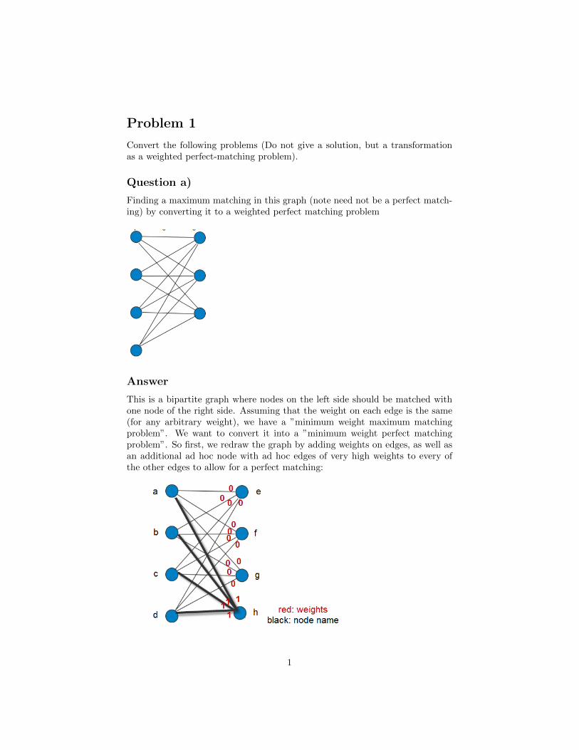
Finding a maximum matching in this graph (note need not be a perfect match-ing) by converting it to a weighted perfect matching problem

Answer

This is a bipartite graph where nodes on the left side should be matched withone node of the right side. Assuming that the weight on each edge is the same(for any arbitrary weight), we have a ”minimum weight maximum matchingproblem”. We want to convert it into a ”minimum weight perfect matchingproblem”. So first, we redraw the graph by adding weights on edges, as well asan additional ad hoc node with ad hoc edges of very high weights to every ofthe other edges to allow for a perfect matching:

1

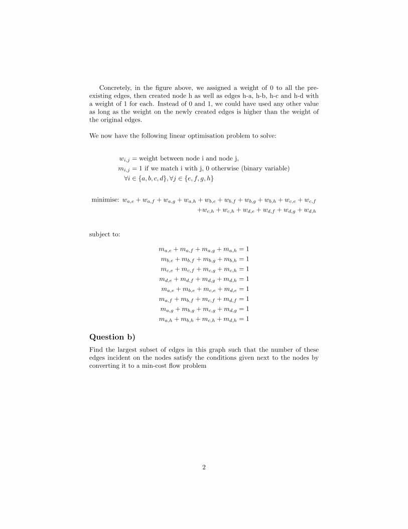
Concretely, in the figure above, we assigned a weight of 0 to all the pre-existing edges, then created node h as well as edges h-a, h-b, h-c and h-d witha weight of 1 for each. Instead of 0 and 1, we could have used any other valueas long as the weight on the newly created edges is higher than the weight ofthe original edges.

We now have the following linear optimisation problem to solve:

wi,j = weight between node i and node j,

mi,j = 1 if we match i with j, 0 otherwise (binary variable)

∀i ∈ {a, b, c, d},∀j ∈ {e, f, g, h}

minimise: wa,e + wa,f + wa,g + wa,h + wb,e + wb,f + wb,g + wb,h + wc,e + wc,f

+wc,h + wc,h + wd,e + wd,f + wd,g + wd,h

subject to:

ma,e +ma,f +ma,g +ma,h = 1

mb,e +mb,f +mb,g +mb,h = 1

mc,e +mc,f +mc,g +mc,h = 1

md,e +md,f +md,g +md,h = 1

ma,e +mb,e +mc,e +md,e = 1

ma,f +mb,f +mc,f +md,f = 1

ma,g +mb,g +mc,g +md,g = 1

ma,h +mb,h +mc,h +md,h = 1

Question b)

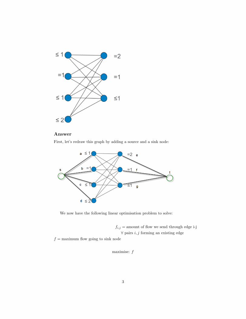
Find the largest subset of edges in this graph such that the number of theseedges incident on the nodes satisfy the conditions given next to the nodes byconverting it to a min-cost flow problem

2

Answer

First, let’s redraw this graph by adding a source and a sink node:

We now have the following linear optimisation problem to solve:

fi,j = amount of flow we send through edge i-j

∀ pairs i, j forming an existing edge

f = maximum flow going to sink node

maximise: f

3

subject to:

(Outgoing flow = incoming flow for each node, except source and sink:)

fe,t + ff,t + fg,t = f

fs,a + fs,b + fs,c + fs,d = −ffs,a − fa,e − fa,f − fa,g = 0

fs,b − fb,e − fb,f − fb,g = 0

fs,c − fc,e − fc,f − fc,g = 0

fs,d − fd,e − fd,f − fd,g = 0

fe,t − fa,e − fb,e − fc,e − fd,e = 0

ff,t − fa,f − fb,f − fc,f − fd,f = 0

fe,g − fa,g − fb,g − fc,g − fd,g = 0

(Sink restrictions:)

me,t = 2

mf,t = 1

mg,t ≤ 2

(Source restrictions:)

ms,a ≤ 1

ms,b = 1

ms,c ≤ 1

ms,d ≤ 2

(All other edges have a max capacity of 1:)

0 ≤ ma,e ≤ 1

0 ≤ ma,f ≤ 1

0 ≤ ma,g ≤ 1

0 ≤ mb,e ≤ 1

0 ≤ mb,f ≤ 1

0 ≤ mb,g ≤ 1

0 ≤ mc,e ≤ 1

0 ≤ mc,f ≤ 1

0 ≤ mc,g ≤ 1

0 ≤ md,e ≤ 1

0 ≤ md,f ≤ 1

0 ≤ md,g ≤ 1

4

Problem 2

Suppose we have a set of 3 sellers labeled a, b, and c, and a set of 3 buyerslabeled x, y, and z. Each seller is offering a distinct house for sale, and thevaluations of the buyers for the houses are as follows.

Describe what happens if we run the bipartite graph auction procedure fromChapter 10, by saying what the prices are at the end of each round of the auc-tion, including what the final market-clearing prices are when the auction comesto an end.

(Note: In some rounds, you may notice that there are multiple choices for theconstricted set of buyers A. Under the rules of the auction, you can choose anysuch constricted set. It’s interesting to consider - though not necessary for thisquestion - how the eventual set of market-clearing prices depends on how onechooses among the possible constricted sets.)

Answer

Round 1The starting prices are 0 for each seller. The preferred-seller graph looks like

that:

5

Set of buyers x, y is constricted to neighbour b, so no perfect matching. Sob increases its price by 1. Prices of a and c are still 0, so no need to reduce theprices.

Round 2With the new prices, the preferred-seller graph looks like that:

Set of buyers x, y is constricted to neighbour b, so no perfect matching. Sob increases its price by 1. Prices of a and c are still 0, so no need to reduce theprices.

Round 3With the new prices, the preferred-seller graph looks like that:

Set of buyers x, y, z is constricted to neighbours b, c so no perfect matching.So b and c increase their price by 1. Price of a is still 0, so no need to reducethe prices.

6

Round 4With the new prices, the preferred-seller graph looks like that:

We now have a perfect matching:

• Buyer x is indifferent between all the sellers: he has a payoff of 3 for eachof them (3-0=3 for a, 6-3=3 for b, 4-1=3 for c).

• Buyer y prefers seller b (payoff of 8-3=5, compared to payoff of 2-0=2 forseller a and payoff of 1-1=0 for seller c)

• Buyer z prefers seller c (payoff of 3-1 = 2, compared to payoff of 1-0 = 0for seller a and payoff of 2-3=-3 for seller b)

• If we attribute b to y (his preferred seller), c to z (his preferred seller) anda to x (one of his preferred seller), then everybody receives his preferredseller and we have a perfect matching at the market clearing prices of 0,3, 1.

Problem 3

Consider a product that has network effects in the sense of our model fromChapter 17. Consumers are named using real numbers between 0 and 1; thereservation price for consumer x when a z fraction of the population uses theproduct is given by the formula r(x)f(z), where r(x) = 1-x and f(z) = z.

Question a)

Lets suppose that this good is sold at cost 1/4 to any consumer who wantsto buy a unit. What are the possible equilibrium number of purchasers of thegood?

7

Answer

We know that

r(x)f(z) = (1− x)z

From Chapter 17, we know that equilibriums can only be found in this modelwhen expectations are rational, i.e. when the expectations of the number ofbuyers is equal to the number of buyers, i.e. z = x. We also know that for anequilibrium to be found, the marginal value for a new individual must be equalto the marginal price (which is here p = 0.25). Then, we must satisfy:

r(x)f(z) ≡ r(z)f(z)

= (1− z)z= z − z2

= 0.25 = p∗

The value of z that satisfies this equation is z = 0.5 = x (i.e. with 50% of themarket purchasing. There is only one solution).

We also have an additional equilibrium at z = x = 0, where no consumerwill buy anything. Since at this point the network effect f(0) = 0, then the valueof the product is 0 ¡ p. This wouldn’t be an equilibrium if a negative numberof consumers could buy the product, but since our model is bounded by thisnon-negativity constraint, z = x = 0 is an equilibrium.

This gives us a total of 2 equilibriums.

Question b)

Suppose that the cost falls to 2/9 and that the good is sold at this cost to anyconsumer who wants to buy a unit. What are the possible equilibrium numberof purchasers of the good?

Answer

Our equation now becomes:

r(x)f(z) ≡ r(z)f(z)

= (1− z)z= z − z2

= 2/9 = p∗

8

The values of z that satisfy this equation are z = 1/3 = x and z = 2/3 = x.

As before, we still have the additional equilibrium at additional equilibriumat z = x = 0. Now, we have a total of 3 equilibriums.

Question c)

Briefly explain why the answers to parts (a) and (b) are qualitatively different.

Answer

The properties of these three equilibriums are not the same, in particular theproperties of the points between each of these equilibriums (i.e. when we don’thave self-fulfilling predictions of z). When we only have three equilibriums likein (b), the second equilibrium represents the tipping point - the minimum levelof expectations you need to reach for your product to converge towards a non-zero equilibrium -, and the third equilibrium represents where your sales will bein the long term if you have reached the tipping point. In our example of (b),what this means is that if you want to launch the product, you need to buildexpectations around a minimum level of 1/3 of the market to be successful, andthat if you are successful you will eventually sell your product to 2/3 of themarket.However, if you only have two equilibriums like in (a), then the tipping pointand the long term point are the same. This doesn’t look like it would make ahuge difference except from the fact that the required effort to reach the tippingpoint is higher, and that the output of that effort is lower as well, but theimplications are actually much bigger than that: maintaining your productabove the tipping point will require a permanently higher effort. If we livein a market with different kinds of shocks and variations over time that couldtemporarily affect our number of consumers (e.g. economic crisis, press scandal,seasonality, etc.), then any loss of consumers below the tipping point needs tobe immediately compensated by some marketing efforts to prevent the modelto start naturally convering towards the lower 0 equilibrium. In other words,we don’t have any margin between the tipping point and the long term stableequilibrium.

Question d)

Which of the equilibria you found in parts (a) and (b) are stable? Explain youranswer.

Answer

As explained in (c), we have for (a):

• Equilibrium z = 0 = x is stable: any upper deviation from the equilib-rium is automatically compensated by a downward pressure and we will

9

converge again towards the same equilibrium. Lower deviations are notpossible since we are already at the lower bound of the model. This equi-librium is the one we reach if we are below the tipping point.

• Equilibrium z = 1/2 = x is semi-stable: any upper deviation from theequilibrium is automatically compensated by a downward pressure andwe will converge again towards the same equilibrium. However, lowerdeviations will lead to a downward pressure and to a convergence towardsthe first equilibrium z = 0 = x. So this equilibrium is only stable onone side, making it much more difficult to maintain that a fully stableequilibrium.

And we have for (b):

• Equilibrium z = 0 = x is stable: any upper deviation from the equilib-rium is automatically compensated by a downward pressure and we willconverge again towards the same equilibrium. Lower deviations are notpossible since we are already at the lower bound of the model. This equi-librium is the one we reach if we are below the tipping point.

• Equilibrium z = 1/3 = x is not stable: both lower and upper deviationswill create a downward/upward pressure which will lead to a convergencetowards a different equilibrium. Staying at this equilibrium requires a lotof stabilization efforts.

• Equilibrium z = 2/3 = x is stable: any lower deviation from the equi-librium is automatically compensated by a upward pressure and we willconverge again towards the same equilibrium. This equilibrium is the onewe reach if we are above the tipping point.

Problem 4

From the Bass Model description (first, relate it to the model and terminologywe did in class) and the data for the Terminator 3 movie, obtain a rollinghorizon estimate of the parameters (using the optimization model described)for a forecast after observing the sales till week 4. Compare them with theestimates in the article.

Answer

Note: I actually use the data of the movie ”The Doctor” instead of ”Termi-nator 3” to answer this question, as allowed by Kalyan on the Hub, since theinput data is more accurate.

The solution to the non-linear Rolling Horizon optimisation model can be foundin the attached file ”Bass model.xlsx”. As shown in the file, by using only thedata of the first 4 weeks to predict the parameters of the model, we obtain:

10

• p = 0.045706097

• q = 0.954293903

• m = 31.7938402

• Sum of squared errors = 2.173489444

where q is the coefficient of imitation, p is the coefficient of innovation, and mis the number of people who will eventually adopt the product.Using the estimates of the article instead, we would have had:

• p = 0.074

• q = 0.49

• m = 34.85

• Sum of squared errors = 9.294759418

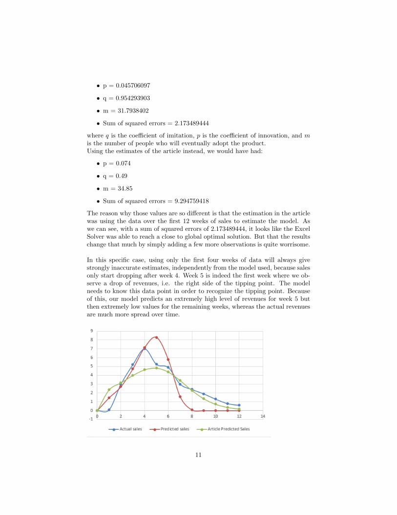
The reason why those values are so different is that the estimation in the articlewas using the data over the first 12 weeks of sales to estimate the model. Aswe can see, with a sum of squared errors of 2.173489444, it looks like the ExcelSolver was able to reach a close to global optimal solution. But that the resultschange that much by simply adding a few more observations is quite worrisome.

In this specific case, using only the first four weeks of data will always givestrongly inaccurate estimates, independently from the model used, because salesonly start dropping after week 4. Week 5 is indeed the first week where we ob-serve a drop of revenues, i.e. the right side of the tipping point. The modelneeds to know this data point in order to recognize the tipping point. Becauseof this, our model predicts an extremely high level of revenues for week 5 butthen extremely low values for the remaining weeks, whereas the actual revenuesare much more spread over time.

11

Of course, the estimates of the article were less good at predicting the salesof the first four weeks (week 4 in particular) since that wasn’t the whole focus ofits objective function, but then much better for the last weeks than our rollinghorizon model (week 7 to 12). In particular, our model predicts levels of salesclose to 0 for weeks 8 to 12, whereas the Bass model using the 12 weeks as inputpredicts some fairly high residual sales.

Still, both models seem to fail at predicting the overall shape of the curve:while their sum of squared residuals have an acceptable value, they both lackthe complexity necessary to explain features such as the angle formed by thecurve at weeks 4-5-6:

But we could use a slightly different variant for the rolling horizon predic-tions. Instead of comparing a model fully predicted from week 1 to week 12,we could use a mixed model where week 1 to week 4 use the actual values, andpredicted values for week 5 to week 12, where week 5’s prediction is based onthe actual sales (instead of the predicted sales) of week 4.The results are shown in the graph below:

12

As we can see, our new prediction curve (in purple) looks very similar to ourold prediction curve (in red), but has the advantage of showing correct valuesfor week 1 to 4. In weeks 5 to 12, the values from the purple curve are slightlydifferent from those of the red curve, sometimes closer to the actual sales andsometimes further. It it not clear whether the mixed prediction curve wouldgive better results that the regular prediction curve since the method we usedstands away from the pure Bass model. The quality of the results might alsodepend on the kind of sales we are trying to predict.

Problem 5

Read the Anatomy of a scientific rumor article by De Domenico, Lima, Mougeland Musolesi and write one paragraph each on the following questions.

Question a)

Summarize the model.

Answer

The model tries to estimate the spreading of information and rumors over timeover a large network, in this case through Twitter. The model was built aroundthe rumor spreading following the discovery of the Higgs Boson in the CERN inJuly 2012, using data acquired directly through the Twitter API. More specif-ically, the model tries to predict the number of active Twitter users at eachpoint of time, where ”active” is defined as whether the user published a Tweetlinked to the news in the given timeframe. The model and its intuition can besummarised with the following equation:

A(t+ 1) = (1− β̃(t))A(t) + (N −A(t)) �λ̃(t) (t)

Where:

13

• A(t+ 1): number of active users at time t+ 1

• A(t): number of active users on the previous period t

• N : total number of users (counting only those who published at leastone tweet related to the topic during the timeframe considered in theexperiment)

• β̃(t): probability at time t that an active user becomes non-active

• �λ̃(t)(t): probability at time t that an inactive user becomes active

Then, the intuition behind that equation becomes:

Number of active users at a given time = (the number of activeusers of the previous period * a dynamic proportionality factor) +(the number of inactive users of the previous period * a dynamicproportionality factor)

What makes this model especially complex is that β̃(t) and �λ̃(t)(t) are not

constants but functions that depend on multiple parameters (not simply ontime). In addition, the model’s behaviour changes depending on the phase ofthe rumour spreading (e.g. before and after the official announcement of thediscovery)

Question b)

How does it differ from the Bass Model?

Answer

This model has many similarities with the Bass model, but is overall a funda-mentally different method.

Both models try to predict the spread of something in a population: of a product(or decision to purchase) for the Bass model, and of information (or the decisionto tweet) for this model; even though products are tangibles and information isintangible, the spread of both can be measured very similarly.Where this model is very different, however, is in its complexity. Just as theBass model, this model expresses the current year’s value as a proportion of lastyear’s values; but here, instead of the constants p and q of the Bass model, weuse the complex function β̃(t) and �λ̃(t)(t) (which I won’t explain in detail).In addition, this model uses Network Data whereas the Bass model uses simplenumeric sales data.Of course, it can be argued that the Bass model could also be extended intosomething more complex where the proportionality parameters are functions(even graph related functions) instead of constants. In this case, the previous

14

arguments would become less valid, but the proportionality constant/functionmultiplies something very different in both models (the (1-F(t)F(t) of the Bassmodel is very different from the A(t) or from the N-A(t) of this model), andthis is something even more fundamental that we cannot consider as a mereextension of the Bass model.

Question c)

How can the model potentially be used in a business application?

Answer

This model could be directly applied in settings where Twitter or similar socialmedia are used as a communication tool, such as viral marketing or publicrelations (notably during a media crisis if the company is negatively impactedby a scandal). This tool not only has the power to increase the managers’understanding of what is happening in the ”social media blackbox”, but canalso help them target the right individuals and choose the right time slots toboost their campaigns/mitigate the impact of bad press. It is especially usefulto know the impact that a certain campaign will have when you need to decideof the budget to attribute to that campaign, or when you need to assess theeffectiveness post-campaign (e.g. using residual analysis to determine whetherthe failure was due to natural variations or bad management).

15