Embed Size (px)
Citation preview

1
Logistic Modeling with Applications to Marketing and Credit Risk in the Automotive IndustryBruce Lund and Keith ShieldsMagnify Analytic Solutions, Division of Marketing Associates
v18b
MSUG conference June 4, 2015

2
Two Goals for this Talk
I. Discuss Concepts and Tools to add to your Logistic Regression Modeling Practice.
II. How to use these Concepts and Tools to: a) Select a Final Logistic Modelb) Build Credit Risk Models (with applications to automotive
finance)

3
A. Briefly: What is Logistic Regression?
An elevator pitch for a very tall building

4
Binary Outcomes Many predictive models in marketing and credit have binary outcomes
… (Buy, Did-Not-Buy), (Defaulted on Loan vs. Paid as Agreed). Outcome of interest (often lower frequency outcome) is “event”, coded
as Y = 1. The “non-event” is coded as Y = 0. In addition to Y we have “predictors” Xk that give information about Y
So, for each customer we want to use predictors Xk to compute the probability that the event occurs … that is … the probability that Y = 1.
But how to do this?

5
How Logistic Model connects predictors to events1. P(Y=1|Xk) is related to Xk’s by taking a weighted sum of the predictors
called “xbeta” and substituting xbeta into the logistic functionP = P(Y=1|Xk) = … the logistic function
where xbeta = β0 + and ’s are unknown parameters
2. We need to find the ’s which best connect the Xk’s to the Y’s
If Y=1, want P big If Y=0, want 1-P big
3. Done by maximizing the likelihood function “L” as a function of ’s Max [ L( X) = (1 - )1- ]

6
PROC LOGISTIC output
DATA WORK;INPUT Y X G$ F;DATALINES;0 0 M 10000 0 F 7501 0 M 501 0 F 370 1 M 8000 1 F 6001 1 M 1001 1 F 75;
Analysis of Maximum Likelihood Estimates
Parameter DF EstimateStandard
ErrorWald
Chi-Square Pr > ChiSqIntercept 1 -3.0018 0.1103 741.2621 <.0001
X 1 0.9220 0.136 45.9666 <.0001G F 1 -0.0023 0.0655 0.0013 0.9716
Chi-Sq 1 df.H0: βX = 0
v.H1: βX ≠ 0
PROC LOGISTIC DATA=WORK DESC;CLASS G;MODEL Y = X G; FREQ F;
1 2
3
betas
Significance Test

7
PROC LOGISTIC output
SCORE CHI-SQUARE makes possible “Best Subset” Model Selection … It ranks ALL possible models, Efficiently. … Discuss Later …
Model Fit StatisticsCriterion Intercept Only And Covariates
AIC 1850.302 1805.330SC 1856.437 1823.735
-2 Log L 1848.302 1799.330Testing Global Null Hypothesis: BETA=0
Test Chi-Square DF Pr > ChiSqLikelihood Ratio 48.9721 2 <.0001
Score 48.6156 2 <.0001Wald 45.9677 2 <.0001
-2 Log L is log (likelihood) (x by -2).
Likelihood Ratio = [-2 Log Lr - (-2 Log Lf)]
Score Chi-Sq approx. LR “computational short-cut”
frf=full, r=restricted
SAS code on web site about Score Chi-Sq

8
B. Creating the Analytic Data Set and Sampling Decisions
We are assuming we have at least semi ”BIG DATA”

9
Training, Validation, Test, #Events, #PredictorsWe will assume the Analytic Dataset has > 1,500 events Split Analytic Data set into Training, Validation, Test data sets
• Training / Validation used together in model fitting • Test used in final evaluation (place in Al Gore’s Lock Box)
One suggestion: Split Analytic Dataset into T,V,T by 40%, 30%, 30%.
How many “predictors” can be in the model?
Guideline: #Events / 10 > Degrees of Freedom used in model • If # Events = 600, then 600/10 = 60 = max d.f. in the model• If C is class predictor with 10 levels, then it uses 9 d.f.

10
Under-Sample Non-Events (Y=0) to avoid long run-times
Assume the non-events are sampled at 1%
1. In PROC LOGISTIC PRIOREVENT = event/(event + 100*nonevents) … [Counts of events and nonevents from sample]
2. In DATA Step after PROC LOGISTIC. Add this adj_P = P / (P + (1 - P) * 100);
3. WEIGHT wgt; in PROC LOGISTIC. Upstream wgt = 100*(Y=0) + (Y=1);
No adjustment needed for P
Likelihood / Wald stat’s are inflated … not reliable for evaluating model.
Only intercept is affected ... but due to random sampling, parameter estimates will change but under-sampling does not create bias. The P’s are wrong but can be adjusted by any of 3 methods (below).

11
C. Preparing, Screening, Transforming of Predictors

12
Preparing, Screening, Transforming of Predictors
Five steps to prepare Predictors before Modeling. Discuss #3.1. Inspect predictors for missing, extremes, errors (EDA)2. Screen (eliminate) predictors with little power3. Transform predictors to achieve best fit4. Remove predictors to avoid multicollinearity5. Test for interactions among X’s and add to candidate list

13
Classify X as: Nominal, Discrete, or Continuous Nominal X … values are “labels” … even if they are numbers(Democrat, Republican, Independent 1, 2, 3 …. But can’t do math)
Discrete X is numeric with a “few” distinct values (e.g. children in HH)Continuous X is numeric with “many” distinct values (money, time, distance)
Is X Discrete or Continuous: Sometimes a “fuzzy” judgement is made.
Recommended Transformations:Nominal and Discrete:
“Optimal” Binning and Weight-of-Evidence transformationContinuous:
Function Selection Procedure (FSP)

14
X Y = 0 Y = 1 Col % Y = 0
Col % Y = 1 WOE= Log(%Y=1/%Y=0)
X=X1 2 1 0.400 0.333 -0.1823X=X2 1 1 0.200 0.333 0.5108X=X3 2 1 0.400 0.333 -0.1823SUM 5 3 1.000 1.000
If X = X3 then X_woe = -0.1823If X = Xk then X_woe = log(%Y=1/%Y=0 | X=Xk)
X: Predictor Y: Target (response)
Weight of Evidence (WOE) Transformation
X is “transformed” to X_woe
Cannot have any “zeros” in Y=0 and Y=1 columns

15
WOE v CLASS v “Dummies”
THREE MODELS – SAME RESULT:PROC LOGISTIC; MODEL Y = X_woe;
OUTPUT OUT = OUT1 P = P1;PROC LOGISTIC; CLASS X; MODEL Y = X;
OUTPUT OUT = OUT2 P = P2;PROC LOGISTIC; MODEL Y = X_dum1 X_dum2 ;
OUTPUT OUT = OUT3 P = P3;
X Y = 0 Y = 1X=X1 2 1X=X2 1 1X=X3 2 1
Y X X_woe X_dum1
X_dum2
0 X1 -0.1823 1 0
0 X1 -0.1823 1 0
1 X1 -0.1823 1 0
1 X2 0.5108 0 1
1 X2 0.5108 0 1
0 X3 -0.1823 0 0
0 X3 -0.1823 0 0
1 X3 -0.1823 0 0
P1 = P2 = P3X_woe uses same d.f. as CLASS X
WOE
CLASS
DUMMY

16
X Y = 0 Y = 1Col % Y = 0
(A)
Col % Y = 1
(B)
Difference(B)-(A)= (C)
WOE= Log(%Y=1/%Y=0)
(D)
IV term(C) * (D)
= IVX=X1 2 1 0.400 0.333 -0.0667 -0.1823 0.0122X=X2 1 1 0.200 0.333 0.133 0.5108 0.0679X=X3 2 1 0.400 0.333 -0.0667 -0.1823 0.0122SUM 5 3 1.000 1.000 IV = 0.0923
Information Value (IV) of X
IV Interpretation0.02 un-predictive0.1 weak0.2 medium0.3 strong
IV measures predictive power• Drop predictors below IV = 0.1 ?
See paper / code by Lin (SGF 2015)

17
Why Bin (Collapse) X Before WOE Coding? WOE coding “burns-up” degrees of freedom (over-fitting) Collapsing levels of X saves “d.f.” (parsimony) but reduces IV But there is a Win-Win … Do the collapsing:
• Usually IV decreases very little in the early stages of collapsing. Sometimes we want X_woe to have monotonic values vs. the
ordering of X … collapse until achieved. X=1, X_woe = -0.5
X=2, X_woe = 1.0X=3, X_woe = 2.3
How to do the collapsing? … next slide gives one approach.

18
DATA EXAMPLE;INPUT X $ Y F;DATALINES;A 0 4A 1 6B 0 8B 1 4C 0 2C 1 5D 0 3D 1 9;
%Best_Collapse(Dataset, X, Y, F, IV, A, , , , WOE)
COLLAPSE (BIN) Target
0, 1Freq.
Mode:(A)ny or
ad(J)acent
IV, LL
SAS WOE code
k -2*Log L IV X_STAT (c) L1 L2 L3 L4
4 50.6084 0.51783 0.68750 A B C D
3 50.6373 0.51441 0.68382 A B C+D
2 51.2002 0.45335 0.65196 A+C+D B
“Optimal” Binning via %Best_Collapse Lund / Brotherton (MWSUG 2013)
Name of Data Set
X_STAT = “c” of PROC LOGISTIC; CLASS X; MODEL Y=X;

19
Function Selection Procedure (FSP) for Continuous X
FSP finds the “best” transformation of a continuous X for use in Logistic Regression
FSP developed in mid-1990’s by P. Royston, W. Sauerbrei, D. Altman, …
Bio-statistical applications
See book Multivariable Model-building (2008) by R & S
See Lund (SGF 2015) for discussion and SAS macros to run FSP
See Appendix for more slides about FSP

20
D. Finding Multiple Candidate Logistic Models for Evaluation and
Comparison

21
Strategy for Selection of Multiple Models Use Schwarz-Bayes Criterion (SBC) to rank ALL (or the most
promising) models … this ranking is based models fitted to the TRAINING data set. … I need to define SBC.
Select, perhaps, 3 to 20 candidate models to be measured on the Validation sample.
Use Validation sample to assess prediction for each of the 3 to 20 models.
Select a final Model. Use TEST for measurement of final model performance.

22
SBC and Ranking ModelsSBC = -2 * LL + log(n)* K … K = d.f. in model and n = sample
A model with more Log Likelihood is better … MORE FIT• A model with Less -2 * LL is better
Adding penalty (log(n)* K) makes -2 * LL an honest measure of FIT The model with smaller SBC is better (better “honest FIT”) All models can be Ranked by their SBC … smaller is better
An alternative is AIC = -2 * LL + 2*K
A CLASS C and C_woe with L levels gives L-1 df when computing K. K includes “1” for “intercept”

23
Concept Developers
Hirotugu Akaike (1927-2009)
Gideon Schwarz (1933–2007)
SBC v. AIC• Both SBC (1978) and AIC
(1973) are firmly grounded in (complex) theory.
• There is no view that one is always superior to the other.
• I think SBC is better for predictive modeling in DM / CR because SBC prevents over-fitting in models with large “n” and many “Xk”
SAS logistic training (with a focus on predictive modeling) uses SBC in generating multiple models for evaluation and comparison

24
SBC and Type 1 Error Probability X is added if: SBC_before > SBC_after …
-2 * LLK + log(n)*K > -2 * LLK+1 + log(n)*(K + 1)D = (-2 * LLK) - (-2 * LLK+1) > log(n)
If n= 10,000, then log(10000) = 9.2 …. Add X if D > 9.2
D is a Chi-Sq with 1 df (if X is not CLASS) under H0: βX = 0
Prob(D > 9.2 | βX = 0) = 0.24% … only ...
0.24% is Type 1 Error probability … with SBC and n=10000 we are unlikely to add an insignificant X
Using AIC: Prob(D > 2 | βX = 0) = 15.7%

25
Finding Candidate Models for Evaluation and Comparison
Three methods … each can be successful
1. Subject Matter Expert fits models by guided trial and error • But not reproducible as a Process
2. Find All (Many) Models using PROC LOGISTIC “Best Subsets” (i.e. SELECTION=SCORE) and rank by (pseudo) SBC
3. Use PROC HPLOGISTIC (SAS/STAT 13.2) to find many good models and rank by SBC.
• Best Subsets is not available in HPLOGISTIC, so what to do?» Use a new method to be explained …

26
Example Data SetThe Slides to follow use Data Set “getStarted” from PROC HPLOGISTIC documentation (n=100)
data getStarted; input C$ Y X1-X10; datalines; D 0 10.2 6 1.6 38 15 2.4 20 0.8 8.5 3.9 F 1 12.2 6 2.6 42 61 1.5 10 0.6 8.5 0.7 D 1 7.7 1 2.1 38 61 1 90 0.6 7.5 5.2
97 more lines
Only Y C X1 X2 X8 are used in Examples. C is nominal.

27
“Backward Plus” with PROC HPLOGISTICods output SelectionDetails = seldtl_b; ods output CandidateDetails = candtl_b;PROC HPLOGISTIC DATA= getStarted; CLASS C; MODEL Y (descending) = X1 X2 X8 C; SELECTION METHOD=BACKWARD
(SELECT = SBC CHOOSE = SBC STOP = NONE) DETAILS=ALL;DATA canseldtl_b; MERGE seldtl_b candtl_b; BY step;PROC PRINT DATA=canseldtl_b;
Variables Removed by Backward
Other Candidates for Removal (the “PLUS”)
SELECT=SBC: Finds the X which gives the smallest SBC if X is removed.

28
Models from Backward Plus
StepNumberInModel
Effect_Removed Effect
Criterion(SBC)
0 5 .1 4 C C 129.141 4 C X1 155.191 4 C X2 159.941 4 C X8 160.362 3 X1 X1 128.192 3 X1 X8 131.612 3 X1 X2 131.743 2 X2 X2 128.383 2 X2 X8 128.704 1 X8 X8 128.22
• Step 1: “C” is removed and new SBC is 129.14
• Step 1: Not chosen candidates X1 X2 X8 and their SBC, if removed.
• Best model: X2 X8

29
If K predictors, then # models = = 2K - 1 (all subsets) Backward Plus provides: 1 + … + K = (K+1)*K/2
All Subsets vs. Backward Plus
Step 0 full Step 1 Step 2 Step 3 Step 4C X1 X2 X8 X1 X2 X8 X2 X8 X8 null
C X2 X8 X1 X2 X2C X1 X2 X1 X8 X1C X1 X8 C X1 C
C X2C X8
SBC removed (in order) C, X1, X2, X8
• Top row are MODELs after Removal
• Blue on white are other “candidates”
• Black on pink are other subsets
K=4=15
=10

30
Go Crazy: Backward-Forward Plus
Step 0 full Step 1 Step 2 Step 3 Step 4C X1 X2 X8 X1 X2 X8 X2 X8 X8 null
C X2 X8 X1 X2 X2C X1 X2 X1 X8 X1C X1 X8 C X8 C
C X1C X2
ALSO: Run HPLOGISTIC “FORWARD” and add Candidate Models • Adds {X1}, {C}, {C X8} but {C X1} and {C X2} are still omitted
SAS code on web site
If K predictors:• B-F Plus finds K models
at each step > 0• Total = K2 - K + 1 • Far fewer than 2K - 1 Does B-F Plus find best SBC model? … usually?

31
B-F Plus … Model RankingVariables in Model from
consolidated F and BAverage
SBCX2 X8 128.237
X8 128.554X2 128.869
X1 X2 X8 130.155X1 X2 131.608
X1 131.822X1 X8 131.922
C X2 X8 155.285C X8 156.167
C 157.357C X1 X2 X8 159.123
C X1 X8 159.939C X1 X2 160.356 X2 X8 still best after
adding Forward
SBC is approximated. SmallDifferences in SBC fromFORWARD and BACKWARD.Take average if model appears in both F and B

32
HPLOGISTIC, CLASS Variable, and WOE Variable Find the top SBC models using CLASS variables in B and F
Now substitute WOE-coded variables for CLASS variables
• Fit and evaluate models on VALIDATION and TEST data sets

33
PROC LOGISTIC “Best Subsets”
Best Subsets using PROC LOGISTIC with SELECTION=SCORE
The Example to follow uses Data Set “getStarted” from HPLOGISTIC documentation (N=100)

34
SELECTION = SCORE Syntax (aka Best Subsets)
PROC LOGISTIC; MODEL Y = <X’s> / SELECTION = SCORESTART=s1 STOP=s2 BEST=b;
look at models with count of predictors between s1 and s2 for each k in [s1, s2] find “b” best-models having k predictors
(What is Best ??… I’ll explain on next slide)
Example: If 4 predictors and START=1 END=4 BEST=3 10 models1 variable models: {X1}, {X2}, {X3}, {X4} take best 32 variable models: {X1 X2}, {X1 X3}, {X1 X4}, {X2 X3}, {X2 X4}, {X3 X4} take best 33 variable models: {X1 X2 X3}, {X1 X2 X4}, {X1 X3 X4}, {X2 X3 X4} take best 34 variable models: {X1 X2 X3 X4} only 1 to take

35
PROC LOGISTIC DATA = getStarted DESCENDING; MODEL Y = <X’s>/ SELECTION = SCORE START = s1 STOP = s2 BEST = b; ?
What is “Best” ?
Short-cut: Don’t need max. likelihood
Testing Global Null Hypothesis: BETA=0Test Chi-Square DF Pr > ChiSq
Likelihood Ratio 48.9721 2 <.0001Score 48.6156 2 <.0001Wald 45.9677 2 <.0001
• “BEST” models have the highest Score Chi-Sq. (among the models having k variables)
• Using Score Chi-Sq is the short-cut making Best-Subsets possible.
• But SBC not available.
Recall: Score Chi-Sq. gives the significance of model

36
CLASS not allowed for SELECTION = SCORECLASS not allowed for “Best Subsets”… must use WOE or Dummies
• Using dummies greatly increases # of subsets … impractical
But Trouble: PROC LOGISTIC is unaware of upstream WOE … df for WOE counted as “1” not “L-1” where WOE has L levels.
Keep in mind.
Other Reasons to use WOE instead of Dummies in Modeling: Some dummies may not be selected in a final model (unintended binning) … applies to Stepwise
and Best Subsets methods Coefficients of dummies may not be ordered in final Model as was expected

37
Here is code to convert C from getStarted to C_woe
Class Variable to WOE
DATA getStarted; SET getStarted;IF C in ( "A" ) THEN C_woe = -0.809318612 ; IF C in ( "B" ) THEN C_woe = 0.1069721196 ; IF C in ( "C" ) THEN C_woe = 0.6177977433 ; IF C in ( "D" ) THEN C_woe = -0.403853504 ; IF C in ( "E" ) THEN C_woe = -1.145790849 ; IF C in ( "F" ) THEN C_woe = -0.809318612 ; IF C in ( "G" ) THEN C_woe = -0.703958097 ; IF C in ( "H" ) THEN C_woe = 0.1069721196 ; IF C in ( "I" ) THEN C_woe = 0.1069721196 ; IF C in ( "J" ) THEN C_woe = 1.4932664807 ;
%Best_Collapse(getStarted, C, Y, 1, IV, A, , , , WOE)

38
Degrees of Freedom for WOE-coded
PROC FORMAT LIBRARY = Work;VALUE $DF“C_woe" = “9“Other = “1”;run;
… Need to do this for all WOE variables available to the Models.

39
Ranking Models from SELECTION=SCORE: SBC vs. ScoreP
Since SBC is not available from SELECTION = SCORE, instead use:ScoreP = -Score Chi-Sq + log(n) * (DF + 1)
… “P” for penalized Score Chi-Square
DF must include the d.f. of WOE-coded predictors(We’ll use the FORMAT)
ScoreP might sort Models differently but top models will be found.

40
Computing ScoreP and Ranking ModelsODS OUTPUT Bestsubsets = Score_Out;PROC LOGISTIC DATA = getStarted; MODEL Y = X1 X2 X8 C_woe/ SELECTION = SCORE START=1 STOP=4 BEST=“big”;
“Big” so ALL models (between s1, s2) are output to Score_Out. Here, “Big” = 6 will work
Need ALL so we can compare all models AFTER corrections are made to DF for WOE’s

41
Computing ScoreP and Ranking Models PROC PRINT DATA = Score_Out;
Obs NumberOfVariables ScoreChiSq VariablesInModel1 1 12.3744 C_woe2 1 4.2986 X8
3-14 omitted omitted omitted15 4 22.3223 X1 X2 X8 C_woe
DATA step reads Score_Out and uses Format DF. to compute:ScoreP = -Score Chi-Sq + log(n) * (DF + 1)

42
Computing ScoreP and Ranking Models PROC SORT DATA = Score_Out; BY ScoreP; PROC PRINT DATA = Score_Out;NumberOfVariables ScoreChiSq VariablesInModel DF ScoreP
2 8.9499 X2 X8 2 4.8656
1 4.2986 X8 1 4.91171 3.9882 X2 1 5.2221
obs 4-14 omitted
3 17.1507 X1 X2 C_woe 11 38.1113
Also Best Model found by HPLOGISTIC Backward +
Candidates
Best
SAS code on web-site

43
Overview: PROC LOGISTIC with SELECTION = SCORE
OVERVIEW: If more X’s 50, then Selection = Score is not feasible (run-time).
Use Selection = Backward Fast to reduce X’s to ~ 30 or less.• If need K = 50 in model, use HPLOGISTIC “B-F Plus”.
Use judgment regarding START, STOP … E.g. why use START = 1?• Then create ALL models by using BEST = “big”
Rank these models by the penalized Score Chi-Square Pick cut-off of “M” models (3 to 20) and measure on Validation
44
E. Evaluation of Models
Now we have 3 to 20 Models to evaluate on the Validation Sample … How do we do this? Discuss after Lunch!
Keith Shields will present. Tell your friends to attend.

45
Evaluation of Models: Credit Scoring Case Study A credit score is a linear combination of credit, contract, and personal attributes of customers
applying for credit.• “Attributes” = “variables” = “predictors” = independent variables
The credit score is a quantification of a customer’s risk of default• The models that spawn credit scores are called risk models
Logistic regression models are at the root of most credit scores• Per Wiki: Although logistic (or non-linear) probability modelling is still the most popular means by which to
develop scorecards, various other methods offer powerful alternatives, including MARS, CART, CHAID, and random forests.
Credit risk models are a good case study for model evaluation because?• Measures of “separation” can be directly tied to business results• Regulation: OCC and CFPB have almost “institutionalized” the risk model development and validation process

46
Brief Background on Credit Scoring
Bill Fair, Earl Isaac…”FICO”• Credit Scoring System• FICO Scores
Equifax “Beacon”, Experian “PLUS”, Trans Union “TransRisk”, Vantage Score
Custom credit risk scores• Many lenders now view this as a core function• Better capture the nuances of an asset class

47
Custom Credit Scores The FICO Score is tuned to predict the likelihood of a customer going
90+ DQ or default on any trade in the next 24 months. Most generic scores are like this.
Generic scores offer a shadow of what auto lenders are most interested in: the likelihood a customer will have his vehicle repossessed• Thus much of the value of a custom risk model lies in the customization of the
target variable.• The quality of a risk model tends to be more dependent on how we define GOOD
and BAD than it is on methodology.• Next slide…

48
Custom Auto Risk Models: Target Variable Example
BAD• Repossession• Charge-off or 90+ day delinquent
INDETERMINATE• 60+ days delinquent• Rewritten or rehabilitated
GOOD• All others
Target = 1 if BAD Target = . if INDETERMINATETarget = 0 if GOOD

49
The Risk Model Separates Goods and Bads
where: G is a good
B is a bad
G
GGG
GGG
G
GG
G
G
GB
BBB B
B B
BB
freq
uenc
y
credit score
"Non-payers"
"Payers"
G
low riskhigh risk
B BBBBB
BBBBBB
G
BB
GGG
G
G
GG
G
G
G
G
G
G
GG
G
G
G
GGG
G
There are several measures that tell us how well the risk model accomplishes what is shown below. We’ll discuss all of them later…
K-S (Kolmogorov-Smirnov) Statistic C-stat (Area under ROC curve…aka AUC) Gini index Lorenz Curves

50
How Lenders Separate Their Goods and Bads Has Become The Subject of Much Scrutiny…
The rise of custom, proprietary risk models has given rise to process and regulation.
From the OCC document entitled “SUPERVISORY GUIDANCE ON MODEL RISK MANAGEMENT”…
• …the term model refers to a quantitative method, system, or approach that applies statistical, economic, financial, or mathematical theories, techniques, and assumptions to process input data into quantitative estimates.
• A model consists of three components: an information input component, which delivers assumptions and data to the model; a processing component, which transforms inputs into estimates; and a reporting component, which translates the estimates into useful business information.
• Next slide…

51
The Logistic Regression “Processing Component”
When we use logistic regression to build a risk model, our “processing component” is this (note: “PD” is the probability of default):
𝑃𝐷=1
1+𝑒−[𝛽0+𝛽1𝑥1+𝛽2𝑥2+…+𝛽𝑛 𝑥𝑛 ]
And x1, x2, …, xn are obviously independent variables, or “attributes”

52
Some Important “Attributes” of the Auto Finance CustomerSome things never change (these are always strong predictors): Credit Score Loan-to-Value Ratio (LTV)
• Insert diatribe on 2008 mortgage disaster
Payment-to-Income Ratio (PTI) Revolving Utilization (Balance on credit cards divided by high credit limit on credit cards) Recent Credit Inquiries Number of recently opened trade lines Number of trade lines reported satisfactory APR
Big Data beginning to manifest itself in auto risk models… Number of addresses attributable to the SSN Number of evictions Number of real estate properties ever owned Indicator for active phone listing at stated address

53
Why Is Dr. Lund’s Presentation So Relevant? It removes some of the “judgmental” element from the risk model
development process, an element the OCC specifically calls out in “SUPERVISORY GUIDANCE ON MODEL RISK MANAGEMENT”…• Model development is not a straightforward or routine technical process. • The experience and judgment of developers, as much as their technical
knowledge, greatly influence the appropriate selection of inputs and processing components.
• …a considerable amount of subjective judgment is exercised at various stages of model development, implementation, use, and validation.
• It is important for decision makers to recognize that this subjectivity elevates the importance of sound and comprehensive model risk management processes.

54
Evaluation of Competing Auto Subprime Models A subprime auto lender has split its customer base into 5 segments and they have
one champion model per segment. Those champion models come from a process similar to the one Dr. Lund presented.
• Segment 1: Clean (Worst status ever on a trade <=150 days late)» Champion model K-S = 35.1
• Segment 2: Dirty (Worst status ever on a trade >=180 days late) Texas» Champion model K-S = 26.4
• Segment 3: Dirty (Worst status ever on a trade >=180 days late) California» Champion model K-S = 29.0
• Segment 4: Dirty (Worst status ever on a trade >=180 days late) Other» Champion model K-S = 30.6
• Segment 5: Missing bureau report» Champion Model K-S = 24.0

55
But What is a K-S? Kolmogorov-Smirnov test statistic…tests the
null hypothesis that two distributions are the same.
For 2 cumulative distribution functions f(score) and g(score):
• KS=max(|B(score)-G(score)|, for all values of score)
• B(score) is the CDF of the bads and G(score) is the CDF of the goods
The magnitude of the KS gives us a good idea of how well the model separates and ranks the risk.
50 80110
140170
200230
260290
320350
380410
440470
500530
560590
0%10%20%30%40%50%60%70%80%90%
100%
75%
17%
K-S Test Statistic
B(score) G(score)
Custom Score
Cum
ulati
ve D
istrib
ution
KS=57

56
SAS Code for K-Sproc npar1way data=validation; var custom_score; class GOOD_indicator; by segment; output out=ksa; run; data ks; set ksa(keep=_var_ _d_ segment in=a);
KS_CUSTOM_SCORE = _D_;drop _D_;
run;proc print data=ks noobs; run;
Computes the K-S of the champion model…
The output looks like this…
Segment _VAR_ KS_CUSTOM_SCORE
Segment 1 CUSTOM_SCORE 0.35109
Segment 2 CUSTOM_SCORE 0.26366
Segment 3 CUSTOM_SCORE 0.28996
Segment 4 CUSTOM_SCORE 0.30608
Segment 5 CUSTOM_SCORE 0.24055
57
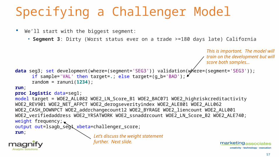
Specifying a Challenger Model We’ll start with the biggest segment:
• Segment 3: Dirty (Worst status ever on a trade >=180 days late) California
data seg3; set development(where=(segment='SEG3')) validation(where=(segment='SEG3')); if sample='VAL' then target=.; else target=(g_b='BAD'); random = ranuni(1234);run;proc logistic data=seg1; model target = WOE2_ALL082 WOE2_LN_Score_B1 WOE2_BAC071 WOE2_highriskcreditactivity WOE2_REV901 WOE2_NET_AFPCT WOE2_derogseverityindex WOE2_ALE801 WOE2_ALL062 WOE2_CASH_DOWNPCT WOE2_addrchangecount12 WOE2_BYRAGE WOE2_liencount WOE2_ALL001 WOE2_verifiedaddress WOE2_YRSATWORK WOE2_ssnaddrcount WOE2_LN_Score_B2 WOE2_ALE740;weight frequency;output out=lsagb_seg1 xbeta=challenger_score;run;
This is important. The model will train on the development but will score both samples…
Let’s discuss the weight statement further. Next slide.

58
The Utility of the Weight Statement in Proc Logistic… Typical use: weight the population back to the population % of GOOD and BAD
• Common practice: sample down the GOODS so that the sample has a 50/50 distribution of GOODS and BADS
• So if we sampled 10% of the GOODS and 100% of the BADS, the weight variable, FREQUENCY is calculated as follows:
» If good_indicator = 1 then FREQUENCY = 10; else FREQUENCY = 1;
We can affect our reject inference through the weight statement. We infer the performance of the rejects through a method called fuzzy augmentation.
• What is a reject inference? Slide 57.• What is fuzzy augmentation? Slide 58.

59
A Note on Reject Inference… Consider the distribution of GOODS and BADS for all applicants:
If we only approve applications with a score of S or greater, then the shaded area represents the applicants that will go into the development sample. The resulting overrepresentation of goods is known as a “selection bias”.
There are a handful of popular methods for inferring the performance of rejects and thus correcting the selection bias problem. We broadly refer to this step in the risk model development process as the “reject inference”.
60
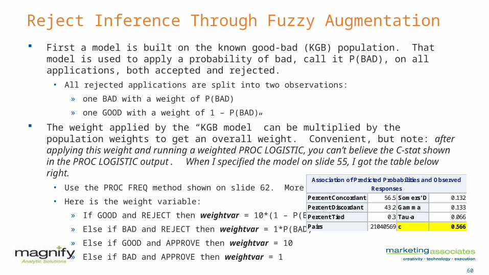
Reject Inference Through Fuzzy Augmentation First a model is built on the known good-bad (KGB) population. That model is used to apply a probability
of bad, call it P(BAD), on all applications, both accepted and rejected.• All rejected applications are split into two observations:
» one BAD with a weight of P(BAD)
» one GOOD with a weight of 1 – P(BAD)
The weight applied by the “KGB model” can be multiplied by the population weights to get an overall weight. Convenient, but note: after applying this weight and running a weighted PROC LOGISTIC, you can’t believe the C-stat shown in the PROC LOGISTIC output. When I specified the model on slide 55, I got the table below right.
• Use the PROC FREQ method shown on slide 62. More on that later.
• Here is the weight variable:
» If GOOD and REJECT then weightvar = 10*(1 – P(BAD))
» Else if BAD and REJECT then weightvar = 1*P(BAD)
» Else if GOOD and APPROVE then weightvar = 10
» Else if BAD and APPROVE then weightvar = 1
Percent Concordant 56.5 Somers' D 0.132
Percent Discordant 43.2 Gamma 0.133
Percent Tied 0.3 Tau-a 0.066
Pairs 21040569 c 0.566
Association of Predicted Probabilities and Observed
Responses

61
After Specifying the Challenger Models… proc npar1way data=validation; var custom_score challenger_score; class GOOD_indicator; by segment; output out=ksa; run; data ks; set ksa(keep=_var_ _d_ segment in=a);
KS_SCORE = _D_;drop _D_;
run;proc print data=ks noobs; run;
Computes the K-S of the champion and challenger…
The output looks like this…
Segment _VAR_ KS_CUSTOM_SCORE
Segment 1 CUSTOM_SCORE 0.35109
Segment 1 CHALLENGER_SCORE 0.3523
Segment 2 CUSTOM_SCORE 0.26366
Segment 2 CHALLENGER_SCORE 0.27432
Segment 3 CUSTOM_SCORE 0.28996
Segment 3 CHALLENGER_SCORE 0.29436
Segment 4 CUSTOM_SCORE 0.30608
Segment 4 CHALLENGER_SCORE 0.31262
Segment 5 CUSTOM_SCORE 0.24055
Segment 5 CHALLENGER_SCORE 0.27428
This is a big improvement. We’d like to know what it means to credit losses.

62
Other Measures of Rank Ordering: C-Stat The C-Stat, sometimes called concordance, is the
probability a randomly chosen good scores higher than a randomly chosen bad.
A step-by-step calculation of C-stat…see right.
This statistic is also referred to as the AUC, or “Area Under Curve”, because it is equal to the area under the ROC curve. See graph below.
Suppose that, in our sample, we have 3 goods (G1, G2, G3) and threebads (B1, B2, B3). Further suppose that a risk model assigned scoresas follows: (G1, 290) (G2, 392) (G3, 175) (B1, 170) (B2, 175) (B3, 280)
To compute concordance, we make all possible pairwise comparisonsbetween the goods and bads, and count the concordant pairs (A pair is concordant if the score of the good is strictly greater than the scoreof the bad). We note the following concordant pairs: G1 & B1, G1 & B2, G1 & B3, G2 & B1, G2 & B2, G2 & B3, G3 & B1
We say that G3 & B3 are discordant because, in this case, the score of the bad account (280) is greater than that of the good (175). G3 & B2are neither concordant nor discordant, we say they’re tied.
C-Stat is defined as: (# of concordant good, bad pairs) + (.5 * # of tied pairs) total # of good, bad pairs
In the above case:C-Stat = (7 + .5*1) / 9= 83.3%

63
Other Measures of Rank Ordering: Gini Index AUC = Area A + Area B Gini Index = Area A / (Area A + Area C)
• Even more convenient: Gini Index = 2*AUC - 1
0.0%5.3%
10.6%16.0%
21.3%26.6%
31.9%37.2%
42.6%47.9%
53.2%58.5%
63.8%69.1%
74.5%79.8%
85.1%90.4%
95.7%0.0%
10.0%
20.0%
30.0%
40.0%
50.0%
60.0%
70.0%
80.0%
90.0%
100.0%
ROC Curves: All Good-Bad Population
% of Goods (ranked low score to high) = False Positive Rate
% o
f Bad
s (r
anke
d lo
w s
core
to h
igh)
=
True
Neg
ative
Rat
e
C
A
B

64
SAS Code for C-Stat, and Giniproc sort data=validation out=all; by segment; run;proc freq data=validation noprint; weight weightvar;table custom_score*GOOD_indicator / measures; by segment; output out=freqout smdrc; run;data cstat; set freqout(keep=_smdrc_ segment); c = (_smdrc_ + 1) / 2; gini = 2*c -1;run;proc print data=cstat noobs; run;
Computes the C-stat and Gini for the champion model by segment…
The output…note that the Gini is the same as the Somer’s D.
Segment _SMDRC_ c gini
Segment 1 0.48819 0.74409 0.48819
Segment 2 0.38534 0.69267 0.38534
Segment 3 0.40971 0.70485 0.40971
Segment 4 0.40973 0.70487 0.40973
Segment 5 0.31731 0.65866 0.31731

65
SAS Code for ROCods graphics on;proc logistic data=validation descending; model GOOD_indicator = oldscore / outroc=oldroc; run;proc logistic data=validation descending; model GOOD_indicator = score2014 / outroc=newroc; run;
data oldroc; set oldroc;oldsens = round(_sensit_,.001); oldspec = round(_1mspec_,.001);run;proc sql;create table oldroc_summ as select oldspec as spec, max(oldsens) as oldsensfrom oldrocgroup by specorder by spec;quit;
Repeat data step and SQL for newroc dataset, and match by SPEC.
ROC Curve:AUC is “area under curve”. It equals the C-stat.

66
How to Tie the Measurements to Business Results? The Lorenz Curve…
Much like the ROC curve in that the Y-axis is the cumulative % of BADS
The X-axis is the cumulative % of loan applications, ranked from lowest score to highest score.
The highlighted points tell us that if we use the FICO score to exclude the worst 40% of the applicants, we exclude 54% of the BADS.
• Assuming 100 total defaults, this would imply a 14/60 = 23% reduction in defaults at a 60% approval rate (vis-à-vis random decisioning).
If we use the Challenger Model to exclude the worst 40% of the applicants, we exclude 68% of the BADS.
• Assuming 100 total defaults, this would imply a 14/46 = 30% reduction in defaults at a 60% approval rate (vis-à-vis FICO-based decisioning).

67
The Lorenz Curve…an Alternative View
Let’s assume that the default rate would be 20% if we approved everyone.
Further assume that our tolerance for default rate is 10%. So we have to set the approval rate so that we eliminate 50% of the defaults.
If we use the FICO score to exclude the worst 50% of the applicants, we decline 39% of the them.
If we use the custom score to exclude the worst 50% of the applicants, we decline 28% of the them.
Þ We approve (72 / 61 – 1) = 18% more loans without increasing the default rate.

68
Wrap-Up A natural extension of the Lorenz-curve evaluation is the calculation of a cutoff score. There is a lot we can say about cutoff scores but this is, after all, slide #66. So just two
things:• Cutoff scores are useful but becoming a bit dated. Well-directed pricing (APR) analysis is
probably more useful.
• To developing a flexible, nuanced, technology-based repayment plan and a clever marketing hook might even more useful than pricing analysis. Insert diatribe on P2P lending here.
Logistic regression will be very difficult to replace as the most commonly used technology for developing credit risk models. Here are just a few reasons:
• History of good results
• existing statistical analysis software
• embedded processes
• regulation

69
Logistic Modeling with Applications to Marketing and Credit Risk in the Automotive IndustryBruce Lund and Keith ShieldsMagnify Analytic Solutions, Division of Marketing Associates
[email protected]@magnifyas.com
MSUG conference June 4, 2015
Contact Information

70
Appendix
Function Selection Procedure

71
Function Selection Procedure (FSP)Step 1: First translate X, if needed, to be positive. Then compute:
FP1: g(X,p) = β0 + β1 Xp …. There are 8 in FP1
FP2: G(X,p1,p2) = β0 + β1 Xp1 + β2 Xp2 p1 ≠ p2
G(X,p1,p1) = β0 + β1 Xp1 + β2 Xp1 log(X) p1 = p2
… There are 36 in FP2.where Xp are called fractional polynomials:
with “p” from S = {-2, -1, -0.5, 0, 0.5, 1, 2, 3} … “0” for log(x).
FSP does this: Find best (Max Likelihood) transform of X from among FP1 and the best transform from among FP2

72
Function Selection Procedure (FSP)Step 2: “3-Step” Test:• Tells us to: Drop X, or Use X, or Use FP1, or Use FP2• Here are the 3 steps:Test Stat = { - 2Log(L)restricted } - { - 2log(L)full } ~ Chi-Sq.1. 4 d.f. test at “α” level of best FP2 against null model. If test is not significant, drop X
and stop, else continue.
2. 3 d.f. test at “α” of best FP2 against a X (linear). If test is not significant, stop (final model is linear), else continue.
3. 2 d.f. test at “α” of best FP2 vs. best FP1. If test is significant, the final model is the best FP2, otherwise it is the best FP1.

73
Function Selection Procedure (FSP)
G(X,-1,-1) = X-1 + 2 X-1 log(X)• FP1 are monotonic
functions. • FP2 (see graph) can be
non-monotonic.

74
A Check List when Starting the ProjectIn the beginning … important actions are taken: Define the Target variable (“events” and “non-events”) Decide to use Logistic Model (and perhaps other methods) Determine Data Sources, resolve IT issuesThe values of the predictor variables are determined as-of an “obs-date”.
Decide if “obs-date” varies by record or fixed “obs-date” all recordsCompile Analytic Data Set and make important decisions: Whether to “Segment” (e.g. purchase history) … model by Segment Allocation Percents to Training, Validation, Test data sets
• Training / Validation used in model fitting. Test used in final evaluation Whether to Sub-sample the Target non-events … applies to Segments

75
Segmenting the Analytic Data SetA model for each Segment:
Upside: Opportunity to “spread” the logistic probabilities
• May have very different average event-rate across the segments … obtain better lifts
Allows use of variables unique to the segment • e.g. current loan customers applying for new loan vs. never-seen-before customers
Avoids using many interaction variables in a single (no segment) model
Downside: More work (modeling), more maintenance, may cause small sample size issues.