Embed Size (px)
Citation preview
Lean ManufacturingDOING IT RIGHT, THE FIRST TIME
the bi-etl’s
What it is?• Production philosophy derived mostly from the Toyota Production System (TPS)
• ‘making obvious what adds value by reducing everything else’
• ‘reduce waste to improve overall customer value’
http://en.wikipedia.org/wiki/Lean_manufacturing
Waste?Toyota defined 3 types of waste:
• muda
• muri
• mura
(all are Japanese terms)
http://en.wikipedia.org/wiki/Lean_manufacturing
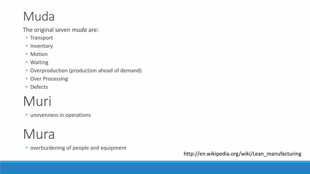
MudaThe original seven muda are:• Transport
• Inventory
• Motion
• Waiting
• Overproduction (production ahead of demand)
• Over Processing
• Defects
Mura
Muri• unevenness in operations
• overburdening of people and equipmenthttp://en.wikipedia.org/wiki/Lean_manufacturing

Area’s of Research Paper’s• Defects
• Just-in-Time
• Inventory
• Over-Processing
• Maintenance

Defects
DefectsFrailty (weak and delicate) or shortcoming in a product
Causes:
• “design defect” is a problem with the product design.
• “manufacturing defect” is a problem that becomes part of the product when it is made.

Defects – White Paper
Zero defect manufacturing as a challenge for advanced failure analysis
Uwe Gäbler – Dr. Ingo Österreicher – Peter Bosk – Christian Nowak Infineon Technologies Dresden GmbH & Co OHG Königsbrückerstr. 180, 01099 Dresden, Germany
Defects - AbstractCustomer requires high quality and reliability
Develop sophisticated strategies for quality learning and continuous improvement in order to meet the challenging expectations of customers towards zero defects.
The goal is no longer to improve quality “just by improving yield” but to apply active quality learning by identifying, analyzing and understanding outliers of any distribution during the whole production and testing processes which would normally not be relevant for yield but are a potential risk for quality.
Advanced failure analysis has also to handle the variations to enable Zero Defect Manufacturing.

Investigate Outliers - ChipMethods :
• SBA (Statistical Bin Alarm)
• PAT (Part Average Testing)
• PEM (Photon Emission Microscope)
• TEM (Transmission Electron Microscope)
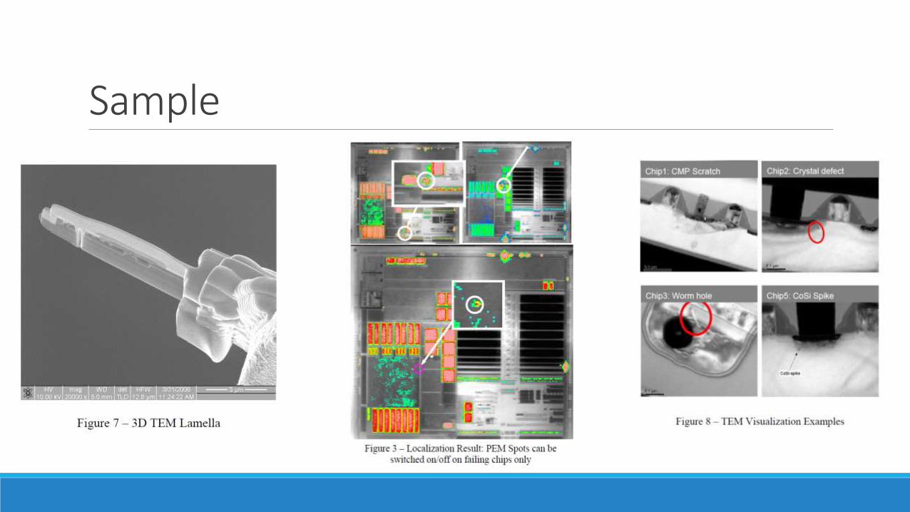
Sample
Defects - ConclusionIn order to enable Zero Defect Manufacturing, Failure Analysis needs to be well-prepared to find the root cause for outliers.

Just-in-Time
What it is?Just in time (JIT) is a production strategy that strives to improve a business' return on investment by reducing in-process inventory and associated carrying costs
The most significant success factor is on-time-delivery to request (OTD-R)
Two models:• Push model
• Pull model

Just-in-Time – White Paper
Staying Ahead of Today’s On-Demand Market: Push Versus Pull Strategies
Robert Rejano
Processes and Applications Advisor
Celestica Supply Chain Managed Services
Push Strategy
Push strategy works from raw material to the consumer’s door, and if the product is unique enough, of high quality, and captures the consumers’ imagination, the product will be successful.
Push strategy enables planned material delivery so that production can meet a specified demand within a defined schedule.
Push strategy works wonderfully when demand is predictable, but there are challenges when forecast accuracy is poor, whether this is due to the ever-changing variables or a failure in S&OP.
Push Strategy – Disadvantage (Bull whip effect)The concept is that as demand is considered at the node that makes contact with the end user, that node will tone up or down the demand based on historical experience.
When the next supplying node performs the same demand adjustment, the resulting modified demand is amplified
As each node optimizes its operation, any buffering done creates a larger gap for the node that supplies it, thus the potential for disconnection becomes an exponential risk
The result can be missed opportunity and/or excess inventory
So product either needs to be “pushed” to the end point at a margin loss or inventory is left unsold and the business incurs costs to hold it.
Pull StrategyUsing an advanced inventory optimization application allows an entire demand chain to be sized in a synchronous optimization cycle
A pull-driven supply chain functions using a series of pull signals to trigger a cascading set of pulls throughout the demand chain.
The bullwhip effect seen in the push model is mitigated by the fact that buffers are optimized as a total system as opposed to independently, so small demand does not become amplified.
Buffers are right-sized, based on a combination of historical forecast performance, statistical models, service level and product life cycle
The size of the buffers complements lean manufacturing principles, correctly positioning buffer stock to manage the gate and better react to unplanned demand fluctuations.
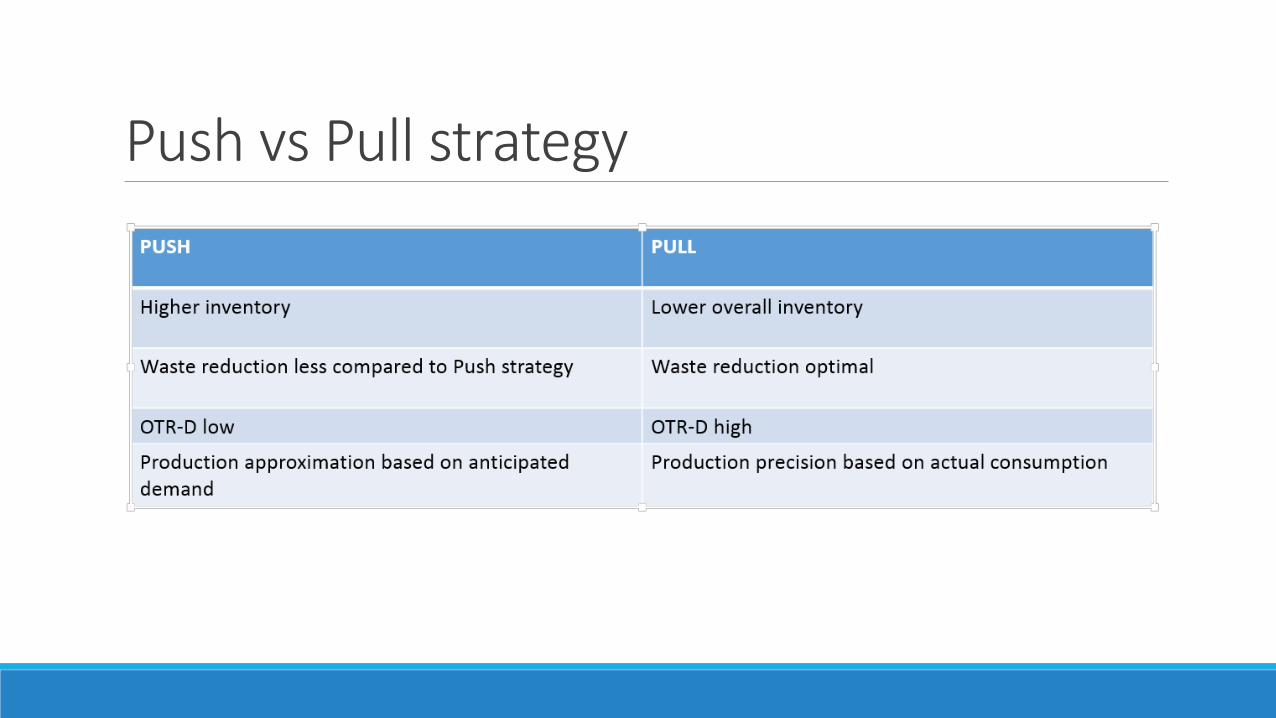
Push vs Pull strategy

Inventory
Inventory – White Paper
Computer Simulation to Manage Lean Manufacturing Systems
Ahmed Deif
Department of Industrial Systems Engineering, University of Regina
Regina, SK, Canada
Inventory
Purpose: Study impact of applying just in time lean policy on a traditional inventory based production system
To have full benefit of lean manufacturing paradigm, systems should undergo substantial change in terms of both culture and infrastructure
The presented model is typical traditional production system which where the production is decided based on demand as well as desired work in progress (WIP) and inventory levels.
JIT is policy that aims to synchronize the pace of the whole system.
Summary
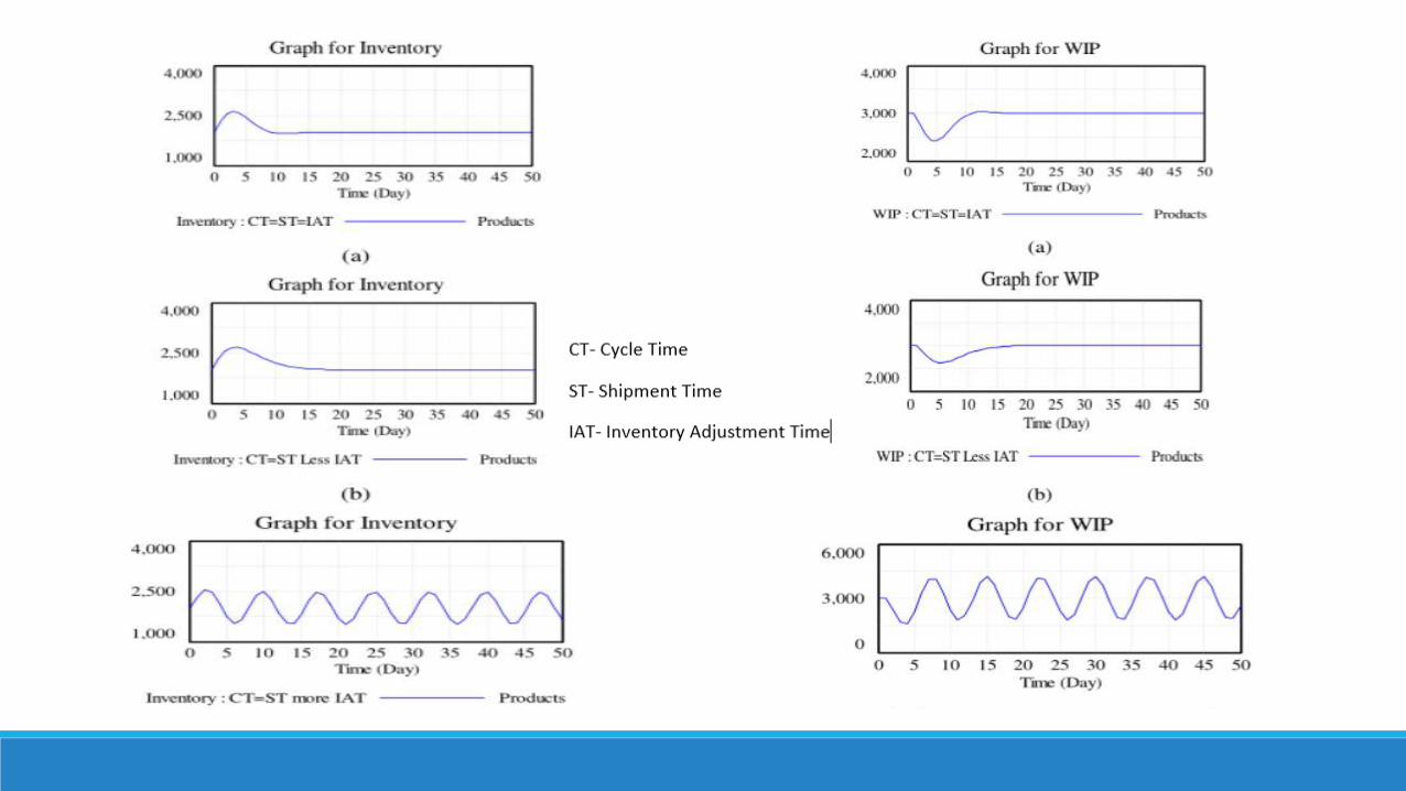
Applying JIT to systems with traditional production and inventory control will not guarantee improvement levels. JIT can bring responsiveness to the manufacturing system, but will also adversely affect the internal system stability.
To benefit for JIT policies and its responsiveness in traditional systems, the inventory adjustment time (IAT) should always be set to be equal to or greater that the cycle time and shipment time.
Traditional systems should start an infrastructure transformation journey to be fully lean. This should happen with gradual implementation of lean tools in parallel.

Over-ProcessingDON’T LET “PERFECT ” STAND IN THE WAY OF “GOOD ENOUGH.”
Over-ProcessingOver-processing is adding more value to a product than the customer actually requires.
Examples:
• Ticket counter reps could put printed tickets on game day into an envelope before handing it to the buyer, who then trashes the envelope (wasted process step and material)
• Painting areas that will never be seen or be affected by corrosion.
• Over polishing parts that would be used internally, no possible viewership.
Over-Processing - Causes
• Bad model/design
• Over-zealous employees
• Misunderstood Customer Requirements
• Not knowing when to stop
Over-Processing - White Paper
The application of systems engineering principles to lean manufacturing to avoid the occurrences of waste generation via defects and over-processing
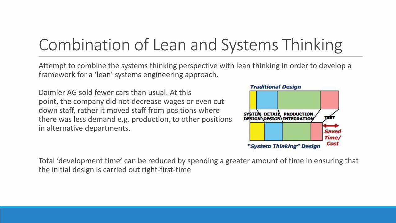
Combination of Lean and Systems ThinkingAttempt to combine the systems thinking perspective with lean thinking in order to develop a framework for a ‘lean’ systems engineering approach.
Daimler AG sold fewer cars than usual. At thispoint, the company did not decrease wages or even cutdown staff, rather it moved staff from positions wherethere was less demand e.g. production, to other positionsin alternative departments.
Total ‘development time’ can be reduced by spending a greater amount of time in ensuring that the initial design is carried out right-first-time
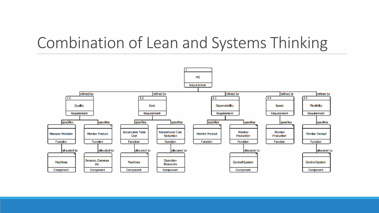
Combination of Lean and Systems ThinkingFrameworks are needed to integrate manufacturing into early system engineering activities that will enable true concurrent engineering of manufacturing and industrial base design concepts
At first, requirements are broken down into lower levels. This gives the designer a big picture view of the whole system and helps to identify anything that may still be missing.
The author suggests that the five performance objectives (quality, speed, dependability, flexibility, cost) can give a good indication of the extent of waste that could occur within the system.
For example, poor performance in the ‘Quality’ dimension will certainly lead us to uncover andeliminate wastes associated with defects, whilst the ‘Speed’ dimension can expose wastes in waiting.
Combination of Lean and Systems Thinking

Maintenance
Maintenance ManagementEquipment Interruption leads to:• Lost Production
• Cost associated with maintenance
• Cost associated with inventory and work-in-process
• Down-Time
• Additional cost associated related to resources
Maintenance – White Paper
A simulation study of predictive maintenance policies and how they impact manufacturing systems
Kaiser, Kevin Michael. "A simulation study of predictive maintenance policies and how they impact manufacturing systems." MS
(Master of Science) thesis, University of Iowa, 2007.
http://ir.uiowa.edu/etd/152.
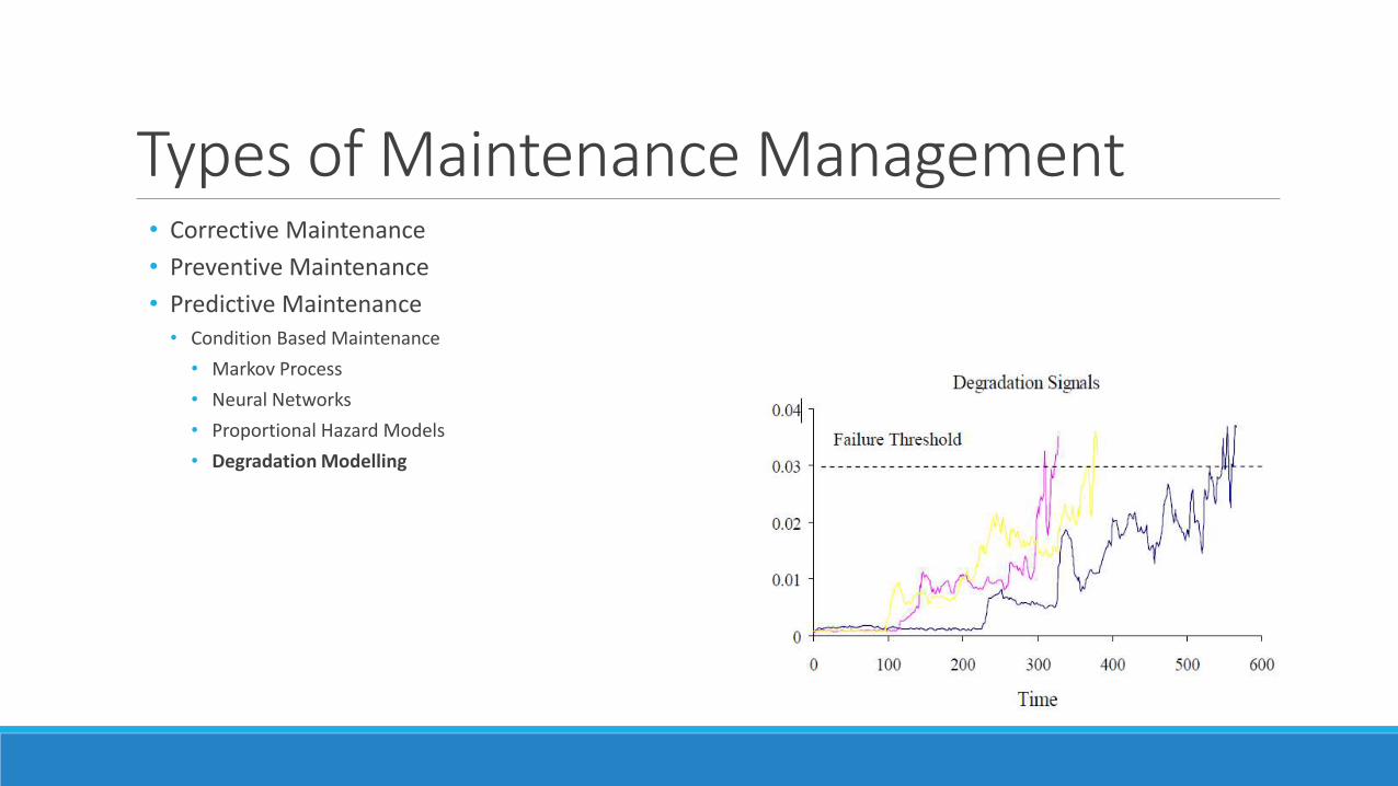
Types of Maintenance Management• Corrective Maintenance
• Preventive Maintenance
• Predictive Maintenance• Condition Based Maintenance
• Markov Process
• Neural Networks
• Proportional Hazard Models
• Degradation Modelling
Maintenance PoliciesPreventive Maintenance
Uses the failure time distribution to calculate the preventive maintenance (PM) interval
Time-based policy
Does not consider the condition or degradation state of the equipment being maintained
Maintenance PoliciesPredictive Maintenance
Utilize condition monitoring information associated with equipment degradation.
The underlying basis of these policies is that the evolutionary trends of the condition-based sensory signals (aka. Degradation signal) can be used to estimate residual life the equipment
The functional form of the signal, depends on the type of component being modeled and represents a relationship between the amplitude of the signal and the operating time.
We assume that the workstations degrade over time and that their degradation is associated with some degradation/performance signal.
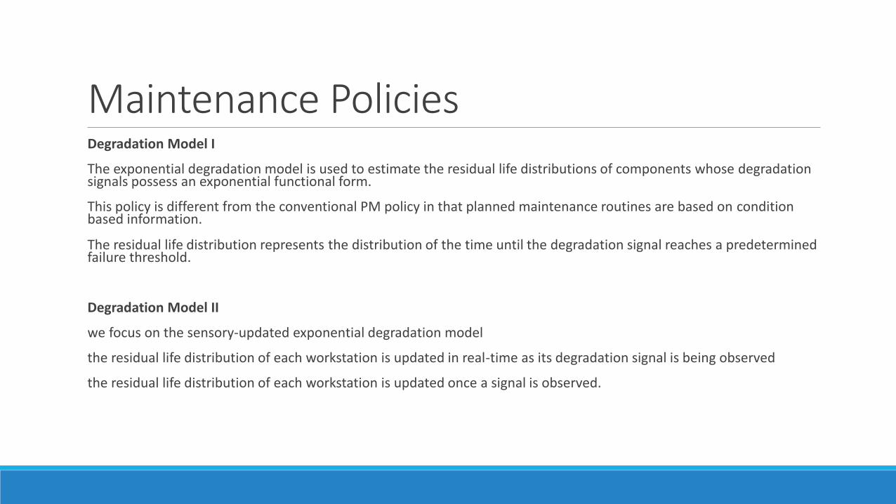
Maintenance PoliciesDegradation Model I
The exponential degradation model is used to estimate the residual life distributions of components whose degradation signals possess an exponential functional form.
This policy is different from the conventional PM policy in that planned maintenance routines are based on condition based information.
The residual life distribution represents the distribution of the time until the degradation signal reaches a predetermined failure threshold.
Degradation Model II
we focus on the sensory-updated exponential degradation model
the residual life distribution of each workstation is updated in real-time as its degradation signal is being observed
the residual life distribution of each workstation is updated once a signal is observed.
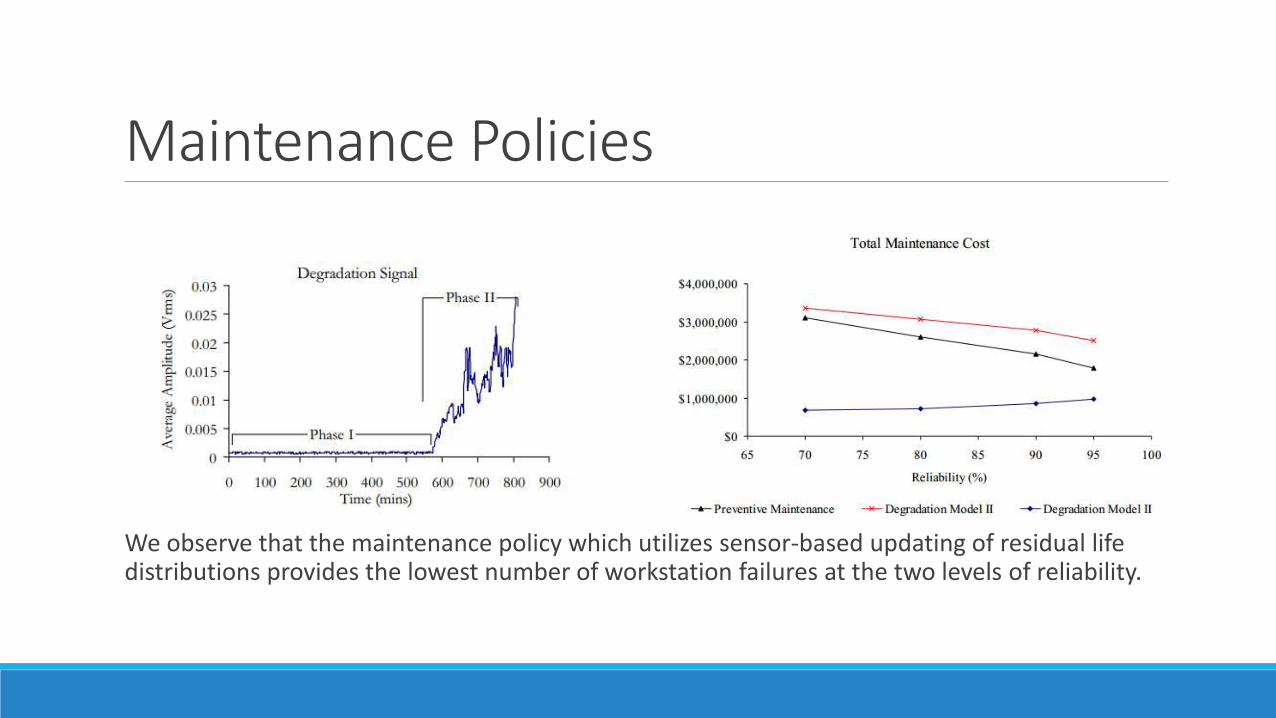
Maintenance Policies
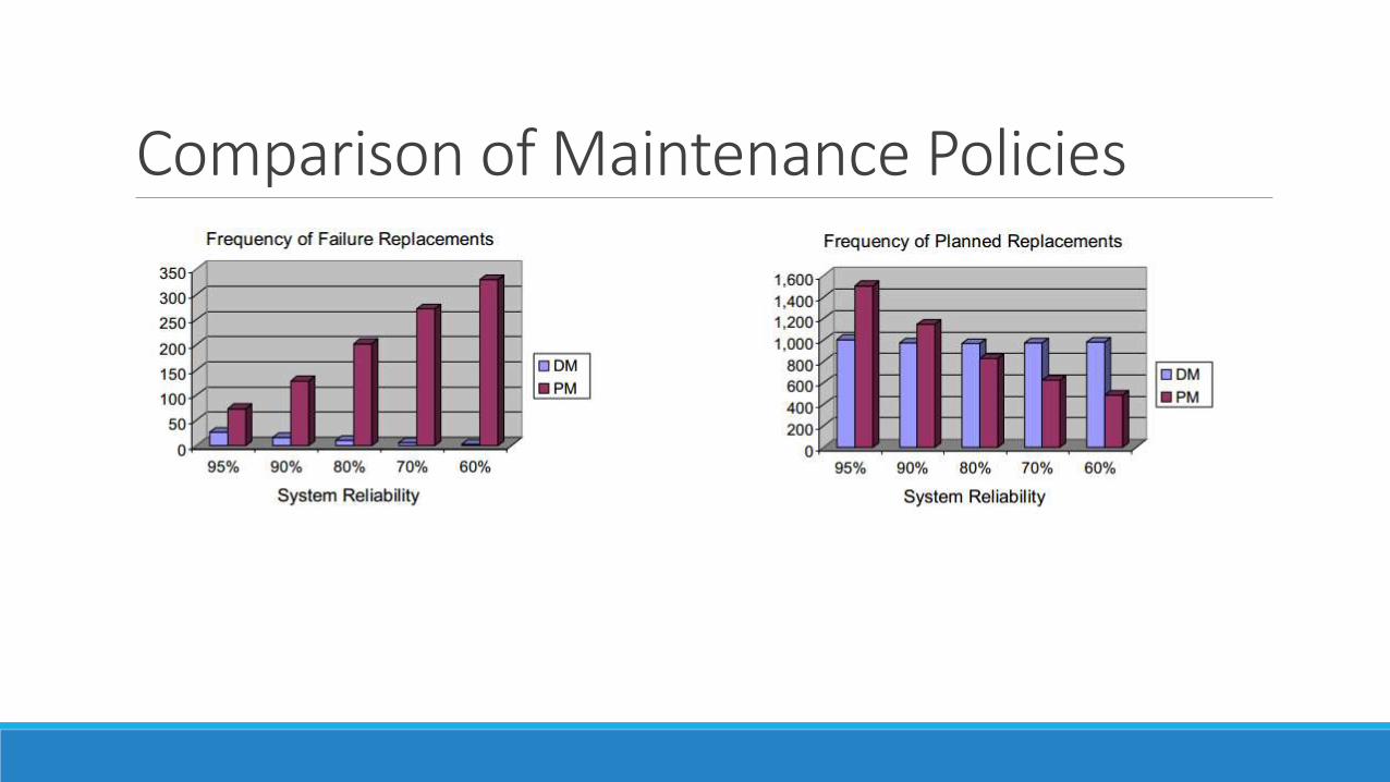
We observe that the maintenance policy which utilizes sensor-based updating of residual life distributions provides the lowest number of workstation failures at the two levels of reliability.
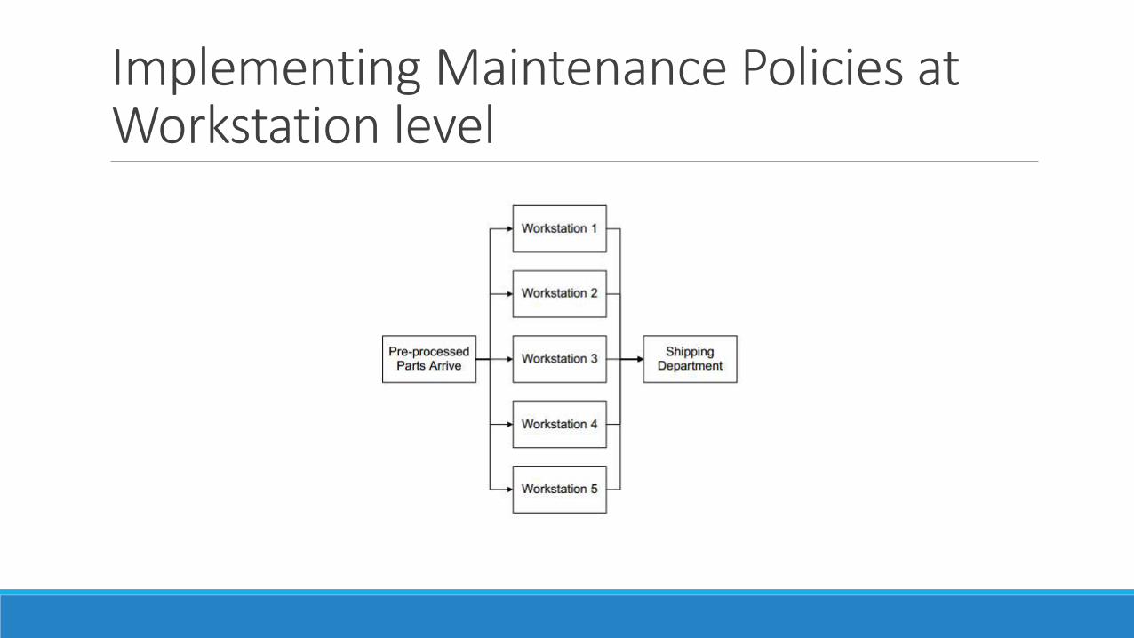
Implementing Maintenance Policies at Workstation level
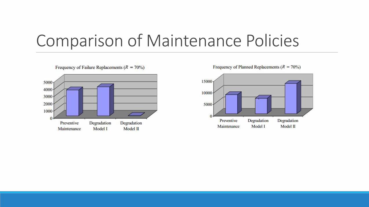
Comparison of Maintenance Policies
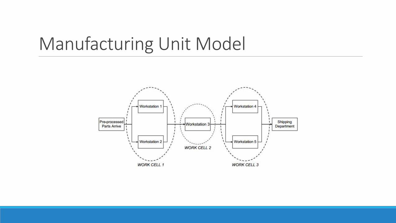
Manufacturing Unit Model
Comparison of Maintenance Policies
Analysis of Maintenance-related decision policiesInvestigate the impact of different replacement and spare parts inventory policies on the performance of a system
Propose a replacement and inventory policy based on the sensory-updated degradation models developed by Gebraeel et al and compare it with a traditional time-based policy that relies on fixed lifetime distributions
Performance is evaluated using -Total cost of system-Average workstation utilization-Throughput
Traditional time-based Replacement and Spare Part Inventory Models
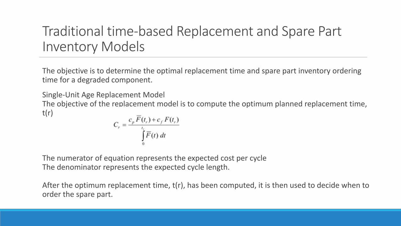
The objective is to determine the optimal replacement time and spare part inventory ordering time for a degraded component.
Single-Unit Age Replacement ModelThe objective of the replacement model is to compute the optimum planned replacement time, t(r)
The numerator of equation represents the expected cost per cycle The denominator represents the expected cycle length.
After the optimum replacement time, t(r), has been computed, it is then used to decide when to order the spare part.
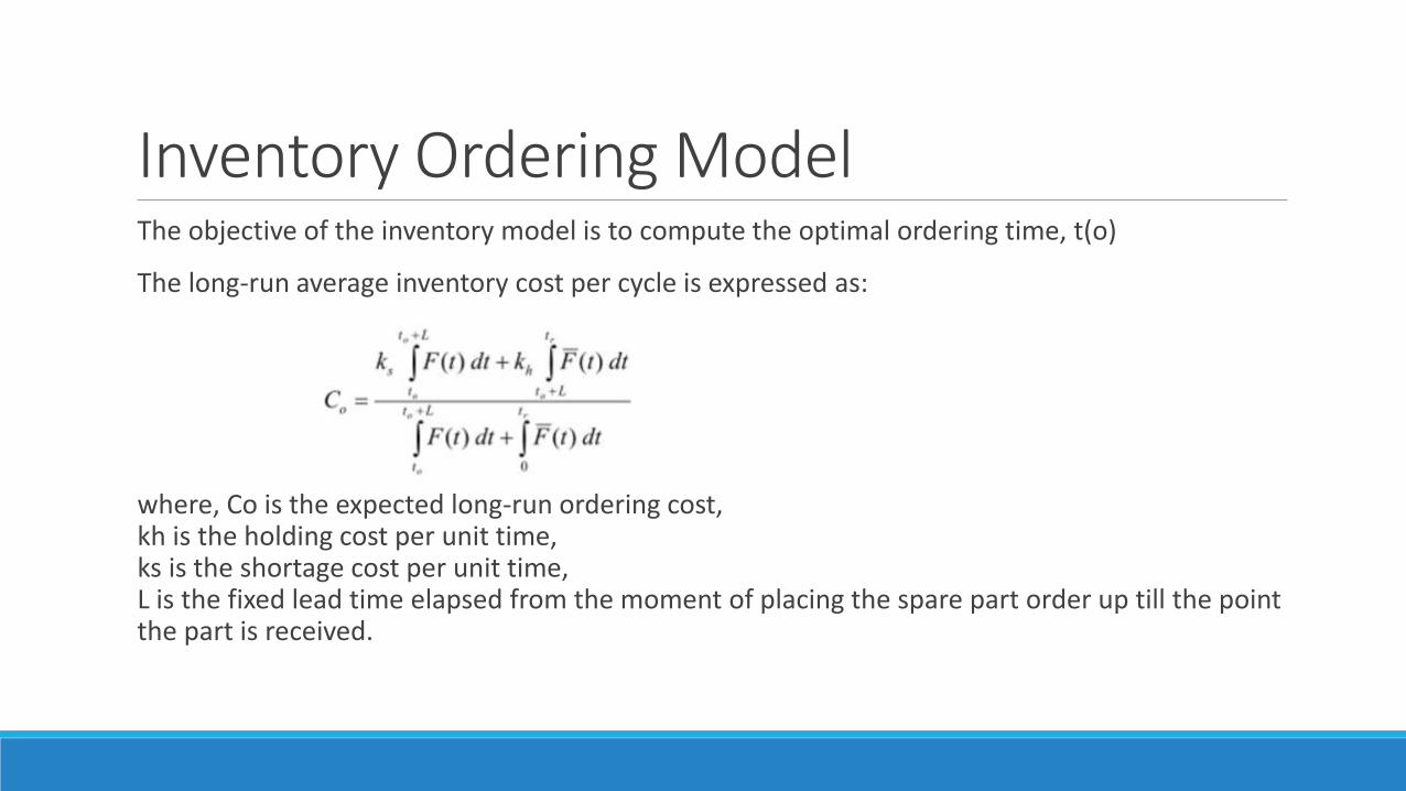
Inventory Ordering ModelThe objective of the inventory model is to compute the optimal ordering time, t(o)
The long-run average inventory cost per cycle is expressed as:
where, Co is the expected long-run ordering cost, kh is the holding cost per unit time, ks is the shortage cost per unit time,L is the fixed lead time elapsed from the moment of placing the spare part order up till the point the part is received.
Traditional time-based model summary
The replacement and inventory models use the failure time distribution of a component to derive their decisions.
Failure time distributions are generally fixed and do not capture the degradation processes that occur prior to failure.
Even when conditional lifetime distributions are evaluated based on the survival time, they remain time-based distributions as opposed to condition-based distributions.
Sensor-driven Replacement and Inventory Policy
It involves replacing these fixed lifetime distributions with sensor-updated residual life distributions that dynamically evolve according to the degradation states of the individual components.
Each time we acquire a signal, the residual life distribution is updated using the degradation modeling framework developed by Gebraeel.
Each time the distribution is updated, the replacement and corresponding inventory ordering times are reevaluated.
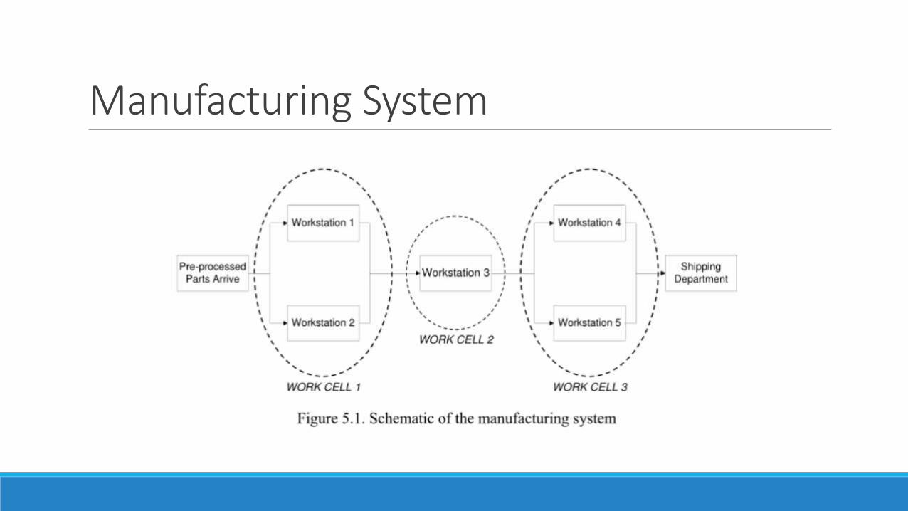
Manufacturing System
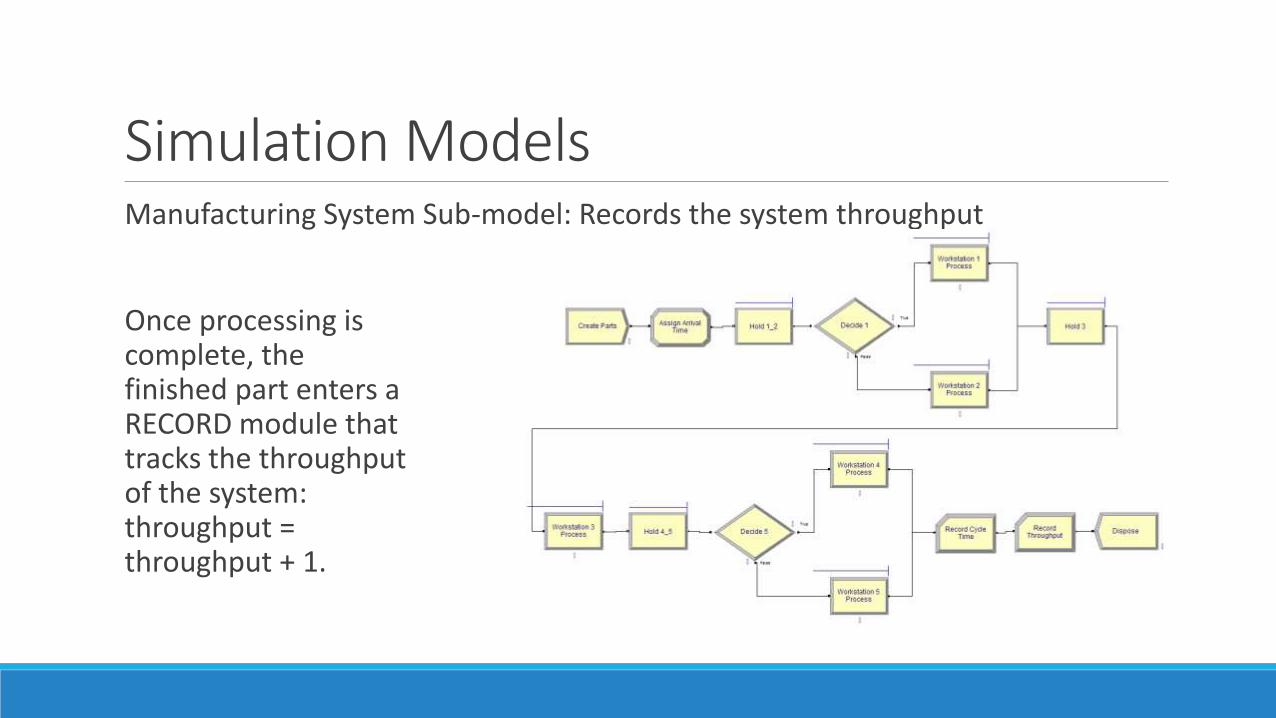
Simulation ModelsManufacturing System Sub-model: Records the system throughput
Once processing is complete, the finished part enters aRECORD module that tracks the throughput of the system: throughput = throughput + 1.
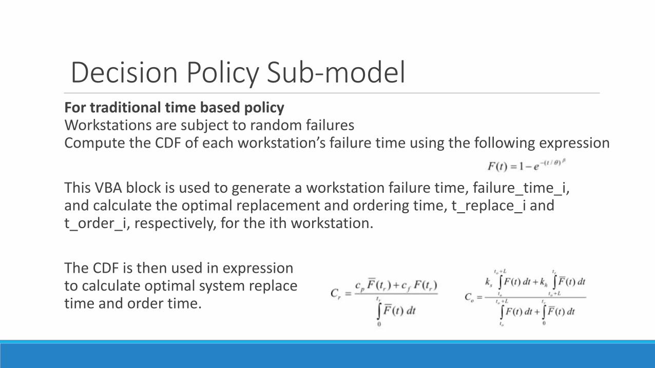
Decision Policy Sub-modelFor traditional time based policyWorkstations are subject to random failuresCompute the CDF of each workstation’s failure time using the following expression
This VBA block is used to generate a workstation failure time, failure_time_i, and calculate the optimal replacement and ordering time, t_replace_i and t_order_i, respectively, for the ith workstation.
The CDF is then used in expressionto calculate optimal system replacetime and order time.
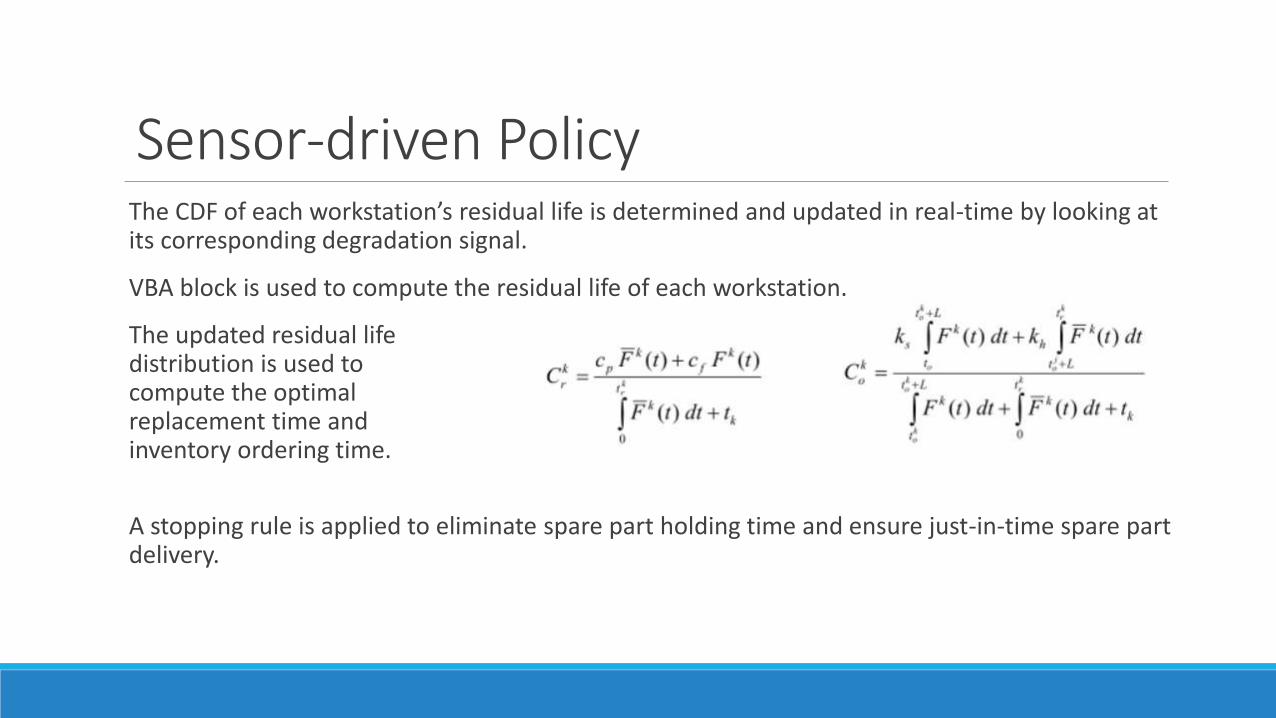
Sensor-driven PolicyThe CDF of each workstation’s residual life is determined and updated in real-time by looking at its corresponding degradation signal.
VBA block is used to compute the residual life of each workstation.
The updated residual life distribution is used to compute the optimal replacement time and inventory ordering time.
A stopping rule is applied to eliminate spare part holding time and ensure just-in-time spare part delivery.
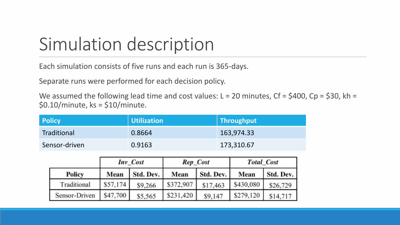
Simulation descriptionEach simulation consists of five runs and each run is 365-days.
Separate runs were performed for each decision policy.
We assumed the following lead time and cost values: L = 20 minutes, Cf = $400, Cp = $30, kh = $0.10/minute, ks = $10/minute.
Policy Utilization Throughput
Traditional 0.8664 163,974.33
Sensor-driven 0.9163 173,310.67
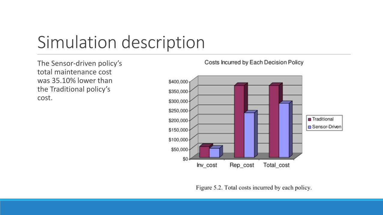
Simulation descriptionThe Sensor-driven policy’stotal maintenance cost was 35.10% lower than the Traditional policy’s cost.

Thank You!
Reference Papers