Embed Size (px)
Citation preview

Thinking in RandomnessStatistical Methods in Finance
Lecture 3
Ta-Wei Huang
December 7, 2016
Ta-Wei Huang Thinking in Randomness December 7, 2016 1 / 28
Table of Contents
In this week, I’d like to tell the story behind the randomness, that is, howto think about our data in an uncertain world.
1 Random Vector and Matrix
2 Why Random Vectors?
3 Random Sample
4 Next Lecture
Ta-Wei Huang Thinking in Randomness December 7, 2016 2 / 28

Table of Contents
In this week, I’d like to tell the story behind the randomness, that is, howto think about our data in an uncertain world.
1 Random Vector and Matrix
2 Why Random Vectors?
3 Random Sample
4 Next Lecture
Ta-Wei Huang Thinking in Randomness December 7, 2016 2 / 28

Table of Contents
In this week, I’d like to tell the story behind the randomness, that is, howto think about our data in an uncertain world.
1 Random Vector and Matrix
2 Why Random Vectors?
3 Random Sample
4 Next Lecture
Ta-Wei Huang Thinking in Randomness December 7, 2016 2 / 28

Table of Contents
In this week, I’d like to tell the story behind the randomness, that is, howto think about our data in an uncertain world.
1 Random Vector and Matrix
2 Why Random Vectors?
3 Random Sample
4 Next Lecture
Ta-Wei Huang Thinking in Randomness December 7, 2016 2 / 28

Random Vector and Matrix
Review: Random Vector
Definition 3.1.1 (Random Vector)
A random vector X =
[X1
...Xn
]is a vector whose elements X1, · · · , Xn are
random variables.
Definition 3.1.2 (Joint Distribution Function)
Let (Ω,F ,P) be a probability space and X = [X1 · · · Xn]′ a random
vector. The joint distribution function of X is defined by
FX(x1, · · · , xn) = P(X1 ≤ x1, · · · , X1 ≤ xn),∀x1, · · · , xn ∈ R.
The joint pdf is given by fX(x1, · · · , xn) = ∂n
∂x1···∂xnFX(x1, · · · , xn).
Ta-Wei Huang Thinking in Randomness December 7, 2016 3 / 28

Random Vector and Matrix
Review: Marginal Distribution and Expectation
Definition 3.1.3 (Marginal Distribution and Expectation)
The marginal distribution of Xi is given by
fXi(xi) =∫· · ·
∫fX(x1, · · · , xn)dx1 · · · dxi−1dxi+1 · · · dxn.
The expectation of Xi is E[Xi] =∫∞−∞ fXi(xi)dxi.
The variance of Xi is var[Xi] = E[(Xi − E[Xi])2].
The covariance of Xi and Xj is
cov[Xi, Xj ] = E[(Xi − E[Xi])(Xj − E[Xj ])].
Now, we’d like to generalize the expectation, variance and covariance of a
random variable to the case of a random vector.
Ta-Wei Huang Thinking in Randomness December 7, 2016 4 / 28

Random Vector and Matrix
Expectation and Covariance Matrix
We can summarize information of means, variances, and covariances of
jointly distributed random variables by the following definitions.
Definition 3.1.4 (Expectation of a Random Vector)
The expectation of a random vector X is E[X] =
[ E[X1]
...E[Xn]
]≡ µ.
Definition 3.1.5 (Covariance Matrix)
The covariance matrix of a random vector X is
cov(X) = Σ = E[(X−µ)(X−µ)′] =
var[X1] cov[X1,X2] ··· cov[X1,Xn]
......
. . ....
cov[Xn,X1] cov[Xn,X2] ··· var[Xn]
.Ta-Wei Huang Thinking in Randomness December 7, 2016 5 / 28

Random Vector and Matrix
Covariance Matrix of Two Random Vectors
Definition 3.1.6 (Covariance Matrix)
Let X =
[X1
...Xp
]and Y =
[Y1
...Yq
]be two random vectors. The covariance
matrix of X and Y is defined as
cov(X,Y) = E[(X−µX)(Y−µY)′] =
cov[X1,Y1] cov[X1,Y2] ··· cov[X1,Yq ]
......
. . ....
cov[Xp,Y1] cov[Xp,Y2] ··· cov[Xp,Yq ]
.Note that here cov(X,Y) = cov(Y,X)′.
Ta-Wei Huang Thinking in Randomness December 7, 2016 6 / 28

Random Vector and Matrix
Propositions
Proposition 3.1.7 (Linear Combination of Random Vector)
Let a = [a1 · · · an]′ be a coefficient matrix and X a random vector. Then
the linear combination a′X is a scalar and
E[a′X] = a′µ =∑n
i=1 aiE[Xi];
cov[a′X] = a′Σa =∑n
i=1
∑nj=1 aiajcov[Xi, Xj ].
Proof.
E[a′X] = E[∑n
i=1 aiXi] =∑n
i=1 aiE[Xi] = a′E[X] = a′µ.
cov[a′X] = E[(a′X− a′µ)(a′X− a′µ)′]
= E[a′(X− µ)(X− µ)′a] = a′E[(X− µ)(X− µ)′]a = a′Σa.
Ta-Wei Huang Thinking in Randomness December 7, 2016 7 / 28

Random Vector and Matrix
Properties of a Covariance Matrix 1-1
Proposition 3.1.8 (Properties of a Covariance Matrix 1)
Let a = [a1 · · · an]′ and An×n be coefficient matrices and X a random
vector with mean µ and covariance matrix Σ. Then,
1 Σ = E(XX′)− µµ′;
2 cov(AX + a) = AΣA′;
3 Σ is a symmetric positive semi-definite matrix.
Proof. To prove (1), we have Σ = E[(X− µ)(X− µ)′]
= E[(X− µ)(X′ − µ′)] = E(XX′ −Xµ′ + µX ′ − µµ′)
= E(XX′)− E(X)µ′ + µE(X)′ − µµ′a = E(XX′)− µµ′.
Ta-Wei Huang Thinking in Randomness December 7, 2016 8 / 28

Random Vector and Matrix
Properties of a Covariance Matrix 1-2
Proof. It is similar to prove (2) by the way mentioned in page 7.
To prove 3, we need the result of spectral decomposition.
Let λ1, ..., λs be the eigenvalues of Σ and e1, ..., es the corresponding
normalized eigenvectors. By the spectral decomposition, we can write
Σ = PΛP ′, where P = [e1 · · · es] and Λ = diag(λ1, ..., λs).
Then, for any n-by-1 vector x, we have
x′Σx = x′PΛP ′x =
n∑i=1
(√λix′ei)
2 ≥ 0.
Therefore, the covariance matrix Σ is a positive semi-definite matrix.
Ta-Wei Huang Thinking in Randomness December 7, 2016 9 / 28

Random Vector and Matrix
Properties of a Covariance Matrix 2
Proposition 3.1.9 (Properties of a Covariance Matrix 2)
Let X,X1,X2 be p× 1 random vectors, a a p× 1 constant vector, Y a
q × 1 random vector, b a q × 1 constant vector, and A,B two q × p
matrices. Then the following properties hold.
1 cov(X1 + X2,Y) = cov(X1,Y) + cov(X2,Y);
2 cov(AX + a, B′Y + b) = Acov(X,Y)B;
3 if X,Y are independent, then cov(X,Y) = 0.
Proof. Skip! Try to prove by your own! (Hint: Use definition.)
Ta-Wei Huang Thinking in Randomness December 7, 2016 10 / 28

Random Vector and Matrix
Random Matrix
Definition 3.1.10 (Random Matrix)
A matrix
Xn×p =
X11 X12 ··· X1p
......
. . ....
Xn1 Xn2 ··· Xnp
is called a random matrix if its each entry Xij is a random variable.
There are two ways to think about a random matrix. We often consider
the column vector as one variable with n outcomes and the row vector as
an observed item with p measurements.
Ta-Wei Huang Thinking in Randomness December 7, 2016 11 / 28

Why Random Vectors?
A Simple Market Model 1
The position in risky securities can be specified as the number of shares of
stock held by an investor.
Definition 3.2.1 (Stock Price)
The price of the share i at time t will be denoted by Si(t).
The current stock price Si(0) is known to all investors
The future price Si(t), t > 0 remains uncertain
The return on stock i at time t is Ri(t) = Si(t)−Si(t−1)Si(t−1) .
Ta-Wei Huang Thinking in Randomness December 7, 2016 12 / 28

Why Random Vectors?
A Simple Market Model 2
The risk-free position can be described as the amount held in a bank
account. As an alternative to keeping money in a bank, investors may
choose to invest in bonds.
Definition 3.2.2 (Bond Price)
The price of one bond at time t will be denoted by B(t) with a fixed
risk-free interest rate r.
Here we do not consider a stochastic risk-free rate.
Example
Assume that the continuous risk-free rate is Rf . Then the bond price at
time t is B(t) = B(0) exp rt.
Ta-Wei Huang Thinking in Randomness December 7, 2016 13 / 28

Why Random Vectors?
A Simple Market Model 3
Our task is to build a mathematical model of a market of financial
securities. A crucial first stage is concerned with the properties of the
mathematical objects involved.
Assumption 3.2.3
The future stock price Si(t) is a random variable with at least two different
values. The future price B(t) of the risk-free security is a known number.
There are still some important assumptions, but we omit it since they are
out of the scope.
Ta-Wei Huang Thinking in Randomness December 7, 2016 14 / 28

Why Random Vectors?
A Simple Market Model 4
Now, suppose an investor forms a portfolio by putting w0 in the risk-free
asset B(t) and w1, ..., wi, ..., wN in risky stocks S1(t), ..., Si(t).
The payoff vector of the bond and stocks is P =
B(t)S1(t)
...SN (t)
.
The weight vector of assets is w′ = (w0 w1 · · · wN ).
Ta-Wei Huang Thinking in Randomness December 7, 2016 15 / 28

Why Random Vectors?
A Simple Market Model 5
The value of that portfolio at time t is
V (t) = w′P = (w0 w1 · · · wN )
B(t)S1(t)
...SN (t)
= w0B(t) +∑N
i=1wiSi(t).
Questions
What is the mean of the value of that portfolio?
What is the variance of the value of that portfolio?
Ta-Wei Huang Thinking in Randomness December 7, 2016 16 / 28
Why Random Vectors?
A Simple Market Model 6
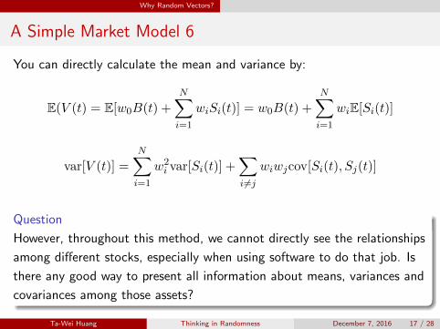
You can directly calculate the mean and variance by:
E(V (t) = E[w0B(t) +
N∑i=1
wiSi(t)] = w0B(t) +
N∑i=1
wiE[Si(t)]
var[V (t)] =
N∑i=1
w2i var[Si(t)] +
∑i 6=j
wiwjcov[Si(t), Sj(t)]
Question
However, throughout this method, we cannot directly see the relationships
among different stocks, especially when using software to do that job. Is
there any good way to present all information about means, variances and
covariances among those assets?
Ta-Wei Huang Thinking in Randomness December 7, 2016 17 / 28

Why Random Vectors?
A Simple Market Model 7
We can also apply the random vector concept to this problem.
E(V (t)) = w′E[P] = (w0 w1 · · · wN )
B(t)E[S1(t)]
...E[SN (t)]
var[V (t)] = w′Σ w =
w′
0 0 ··· 0
var[S1(t)] cov[S1(t),S2(t)] ··· cov[S1(t),SN (t)]
......
. . ....
cov[SN (t),S1(t)] cov[SN (t),S2(t)] ··· var[SN (t)]
w
Ta-Wei Huang Thinking in Randomness December 7, 2016 18 / 28

Why Random Vectors?
Summary
From here, we can clearly see two things.
In classical view, the price bond position B(t) is fixed at any time t.
Since the stock position S1(t), · · · , SN (t) has the feature of
randomness, we assume that the random vector of stock prices
follows a joint normal distribution (a very simple assumption).
Ta-Wei Huang Thinking in Randomness December 7, 2016 19 / 28

Random Sample
Collect the Sample
Suppose that you want to know the profitability of a specific industry in
the world. Then, you need to do the following steps:
1 Find a proxy of the profitability. ⇒ EPS, Profit Margin, etc.
2 Collect a representative ”sample.”
⇒ Random sampling, cluster sampling, etc.
3 Make assumption and then do the statistical modeling.
⇒ Normality assumption, i.i.d assumption, GARCH assumption.
Here, we use mathematical concepts to present the above steps.
Ta-Wei Huang Thinking in Randomness December 7, 2016 20 / 28

Random Sample
Random Sample: One Variable Case 1
Definition 3.3.1 (Random Sample)
If the random variables X1, · · · , Xn ∼ f(x|θ) are independent and
identically distributed (iid), then these random variables constitute a
random sample of size n from the common distribution f(x|θ).
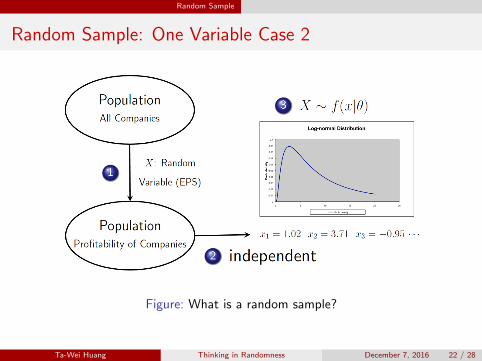
1 For n companies, each of them has an uncertain profitability proxy Xi.
2 X1, · · · , Xn are independently chosen from the population.
⇒ What is the population in this case?
3 Statistical assumptions: assume that X1, · · · , Xn have a common
distribution f(x|θ).
Ta-Wei Huang Thinking in Randomness December 7, 2016 21 / 28
Random Sample
Random Sample: One Variable Case 2
Figure: What is a random sample?
Ta-Wei Huang Thinking in Randomness December 7, 2016 22 / 28

Random Sample
Random Sample: Multivariate Case
Definition 3.3.2 (Random Sample)
Let X =
X11 X12 ··· X1p
......
. . ....
Xn1 Xn2 ··· Xnp
=
X′1
...X′
n
be a random matrix.
We say that X is a random sample if X1, · · · ,Xn are independent and
identically distributed (iid) with joint pdf f(x1, · · · , xp|θ).
Note that each vector Xi = [Xi1 · · · Xip]′ is a bundle of n variables on
a single item i. The definition suggests that
1 The n items are independent and identically distributed.
2 The p variables may have correlation depicted by the joint pdf.
Ta-Wei Huang Thinking in Randomness December 7, 2016 23 / 28

Random Sample
Take a Look at the Dataset
The dataset given below is regarded as a realization of a random matrix X.
X1 X2 · · · Xp
Item 1 x11 x12 · · · x1p
Item 2 x21 x22 · · · x2p...
......
......
Item n xn1 xn2 · · · xnp
Nonparametric analysis: no specific distribution is assigned to
Xi = [Xi1 · · · Xip]′.
Parametric Estimation: Xi = [Xi1 · · · Xip]′ follows a specific
distribution f(x1, · · · , xp|θ) with parameter(s) θ.
Ta-Wei Huang Thinking in Randomness December 7, 2016 24 / 28

Random Sample
Nonparametric Method: Kernel Density Estimation 1
Let x1, · · · , xN be a realization of a random sample X1, · · · , XN . A
natural local estimate of the density function has the form
f(x0) =# xi ∈ B(x0, λ)
Nλ,
where B(x0, λ) is an open ball with center x0 and radius λ.
The above estimator is very naive, and most of time we use another
estimator called Parzen estimate, which is more complicated.
Ta-Wei Huang Thinking in Randomness December 7, 2016 25 / 28

Random Sample
Nonparametric Method: Kernel Density Estimation 2
Here is an simple example. The data x is 1000 random number generating
from a longnormal distribution with mean 1 and standard deviation 0.5.
The following graph shows results of density estimation.
Ta-Wei Huang Thinking in Randomness December 7, 2016 26 / 28
Random Sample
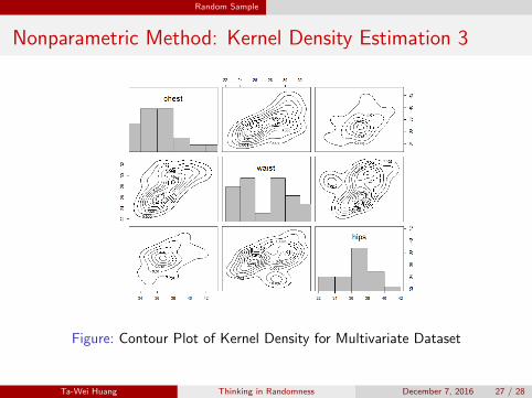
Nonparametric Method: Kernel Density Estimation 3
Figure: Contour Plot of Kernel Density for Multivariate Dataset
Ta-Wei Huang Thinking in Randomness December 7, 2016 27 / 28

Next Lecture
The Next Lecture
In next lecture, I’ll introduce a very popular parametric statistical model -
the linear model.
Ta-Wei Huang Thinking in Randomness December 7, 2016 28 / 28


![(Pseudo) Randomness [2ex]](https://img.pdfslide.us/doc/110x75/61570689a097e25c765040f3/pseudo-randomness-2ex.jpg)