Dmitrii Tihonkih

Department of Mathematics, Chelyabinsk State University, Russian Federation

Artyom Makovetskii

Department of Mathematics, Chelyabinsk State University, Russian Federation

Vladislav Kuznetsov

Department of Mathematics, Chelyabinsk State University, Russian Federation

E-mails: sparsemind@gmail.com, artemmac@csu.ru, k.v.net@rambler.ru

The iterative closest points algorithm and affine

transformations

AIST'2016

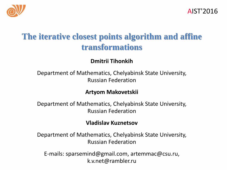
IntroductionThe standard ICP starts with two point clouds fortheir relative rigid-body transform, anditeratively refines the transform by repeatedlygenerating pairs of corresponding points in theclouds and minimizing an error metric.

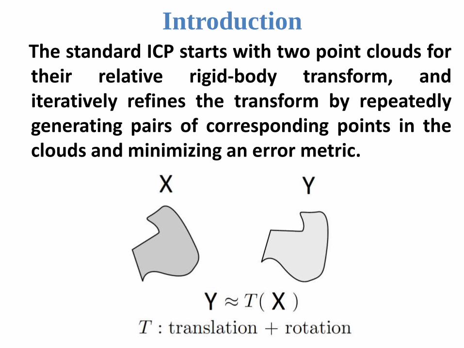
The ICP stages:

1. Selection of some set of points in oneclouds.

2. Matching these points to samples inthe other cloud.

3. Rejecting certain pairs based onlooking at each pair individually orconsidering the entire set of pairs.

4. Assigning an error metric based onthe point pairs.

5. Minimizing the error metric(variational subproblem of the ICP).

Our main focus is on the accuracy of the finalanswer and the ability of ICP to reach thecorrect solution for a given difficult geometry.We consider transformation that hold theangles between lines in the cloud of points.Also we consider the ICP minimizing the errormetric subproblem for the case of an arbitraryaffine transformation.

The matching procedure for sets 𝐗and 𝐘

Let 𝑋 = {𝑥0, … , 𝑥𝑘−1} be an set consist of 𝑘points in ℝ3 and 𝑌 = {𝑦0, … , 𝑦𝑛−1} be an set consist of 𝑛 points in ℝ3. Denote by (𝑥𝑖 , 𝑦𝑗),

𝑥𝑖 ∈ 𝑋, 𝑦𝑗 ∈ 𝑌 the pair of corresponding

points. Note, that each point from 𝑋 and 𝑌 can be included to the set of pairs just one time.

At the beginning the set of pairs is empty. Let 𝑚 ∈ ℕ be a number such that:

3 ≤ 𝑚 ≤ min(𝑛, 𝑘).

1. Consider the following subset 𝑋𝑖 of the 𝑋: 𝑋𝑖 = {𝑥𝑚∗ 𝑖−1 , … , 𝑥𝑚∗ 𝑖−1 +𝑚−1}.

2. Let 𝐶 be a closed piecewise linear curve in ℝ3

that consist of 𝑚 line segments. The 𝑗-th segment connects points 𝑥𝑚∗ 𝑖−1 +𝑗 and 𝑥𝑚∗ 𝑖−1 +𝑗+1.

Denote by 𝛼𝑗 a minimal flat angle that is

constructed by 𝑗-th and (𝑗 + 1)-th segments.Let 𝑉𝑋 be a vector

𝑉𝑋 = {𝛼0, … , 𝛼𝑚−1},

where elements αj, j = 0, … ,m − 1 are

respective angles.

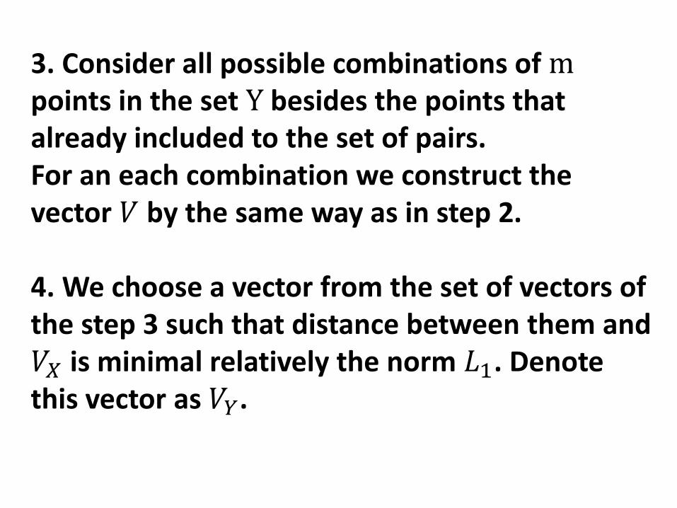
3. Consider all possible combinations of mpoints in the set Y besides the points that already included to the set of pairs. For an each combination we construct the vector 𝑉 by the same way as in step 2.

4. We choose a vector from the set of vectors of the step 3 such that distance between them and 𝑉𝑋 is minimal relatively the norm 𝐿1. Denote this vector as 𝑉𝑌.

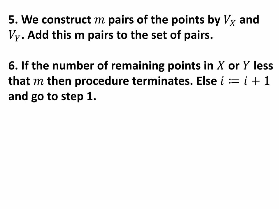
5. We construct 𝑚 pairs of the points by 𝑉𝑋 and 𝑉𝑌. Add this m pairs to the set of pairs.

6. If the number of remaining points in 𝑋 or 𝑌 less that 𝑚 then procedure terminates. Else 𝑖 ≔ 𝑖 + 1and go to step 1.

We use this procedure only as first iteration on the ICP algorithm. Obtained after the first iteration the transformation matrix and the translation vector are used for a second iteration. In the next iterations we use the standard nearest neighbor approach.

The described above approach can good work not for rigid transformation only but for sufficiently wide subset of the affine transformations.

The ICP variational subproblem for

an arbitrary affine transformation

Suppose that the relationship between points in 𝑋 and 𝑌 is done by such a way that for each point 𝑥𝑖 is calculated corresponding point 𝑦𝑖.

The ICP algorithm is offten considered as a geometrical transformation for rigid objects mapping 𝑋 to 𝑌:

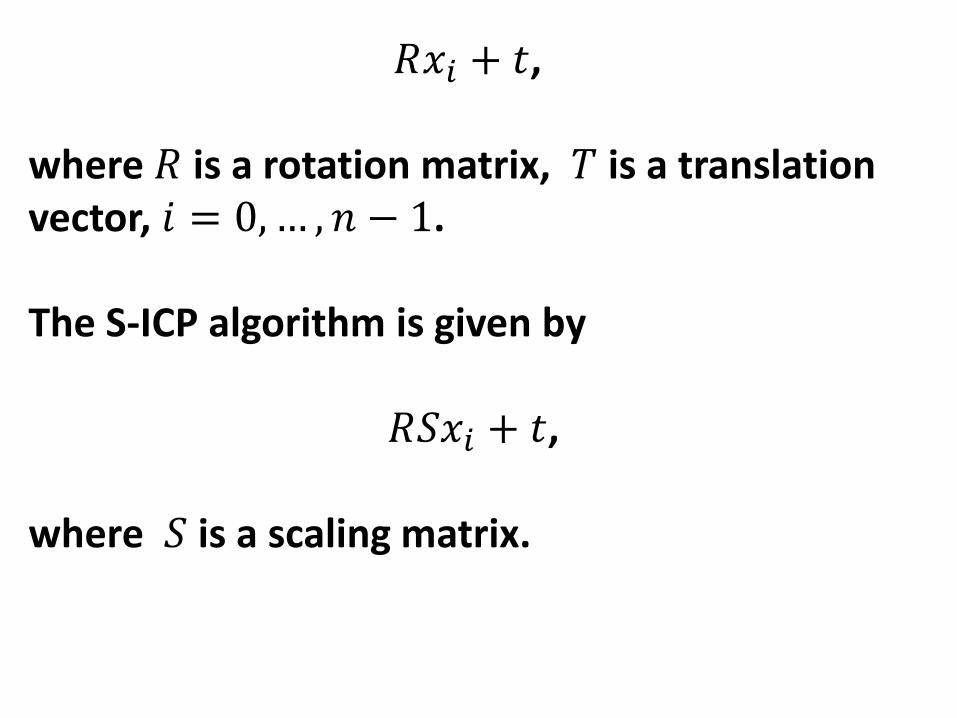
𝑅𝑥𝑖 + 𝑡,

where 𝑅 is a rotation matrix, 𝑇 is a translation vector, 𝑖 = 0,… , 𝑛 − 1.

The S-ICP algorithm is given by

𝑅𝑆𝑥𝑖 + 𝑡,

where 𝑆 is a scaling matrix.

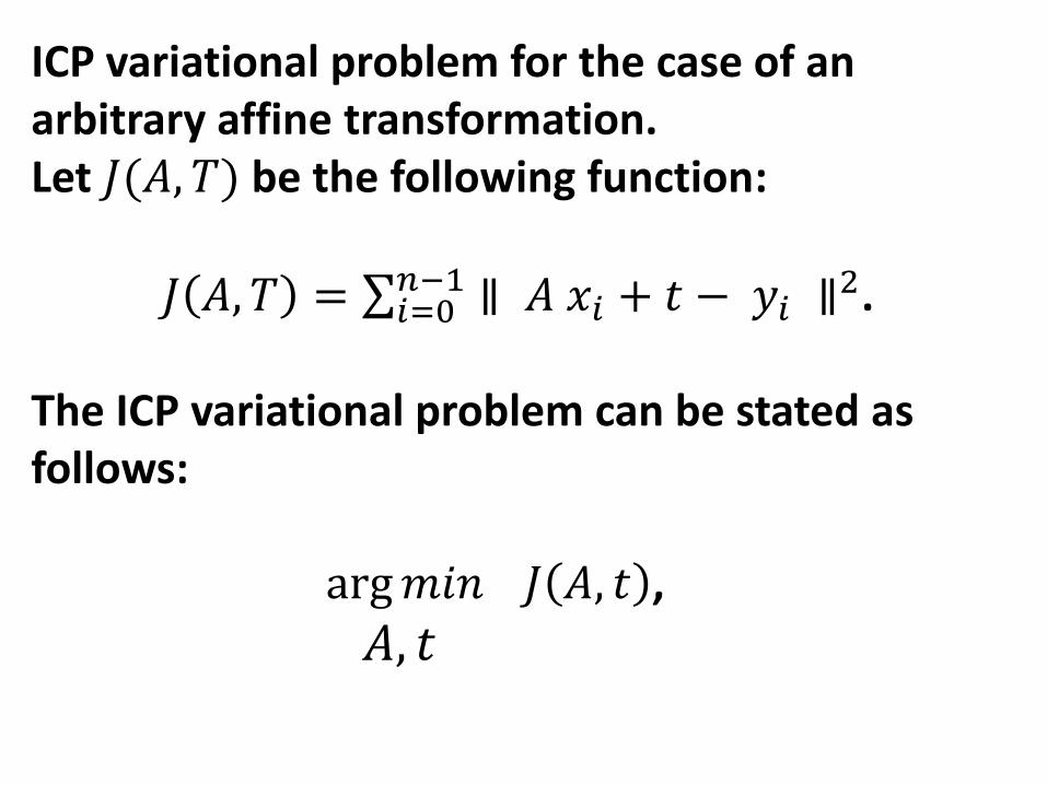
ICP variational problem for the case of an arbitrary affine transformation.Let 𝐽(𝐴, 𝑇) be the following function:

𝐽 𝐴, 𝑇 = 𝑖=0𝑛−1 ∥ 𝐴 𝑥𝑖 + 𝑡 − 𝑦𝑖 ∥2.

The ICP variational problem can be stated as follows:

arg𝑚𝑖𝑛 𝐽 𝐴, 𝑡 ,

𝐴, 𝑡

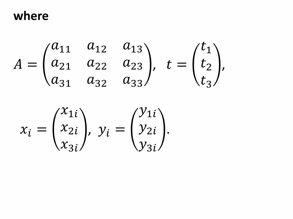
where

𝐴 =

𝑎11 𝑎12 𝑎13

𝑎21 𝑎22 𝑎23

𝑎31 𝑎32 𝑎33

, 𝑡 =

𝑡1𝑡2𝑡3

,

𝑥𝑖 =

𝑥1𝑖

𝑥2𝑖

𝑥3𝑖

, 𝑦𝑖 =

𝑦1𝑖

𝑦2𝑖

𝑦3𝑖

.

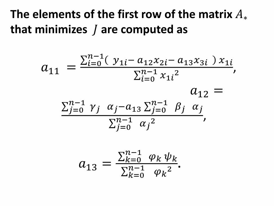
The elements of the first row of the matrix 𝐴∗

that minimizes 𝐽 are computed as

𝑎11 = 𝑖=0

𝑛−1 𝑦1𝑖− 𝑎12𝑥2𝑖− 𝑎13𝑥3𝑖 𝑥1𝑖

𝑖=0𝑛−1 𝑥1𝑖

2 ,

𝑎12 = 𝑗=0

𝑛−1 𝛾𝑗 𝛼𝑗−𝑎13 𝑗=0𝑛−1 𝛽𝑗 𝛼𝑗

𝑗=0𝑛−1 𝛼𝑗

2 ,

𝑎13 = 𝑘=0

𝑛−1 𝜑𝑘 𝜓𝑘

𝑘=0𝑛−1 𝜑𝑘

2 .

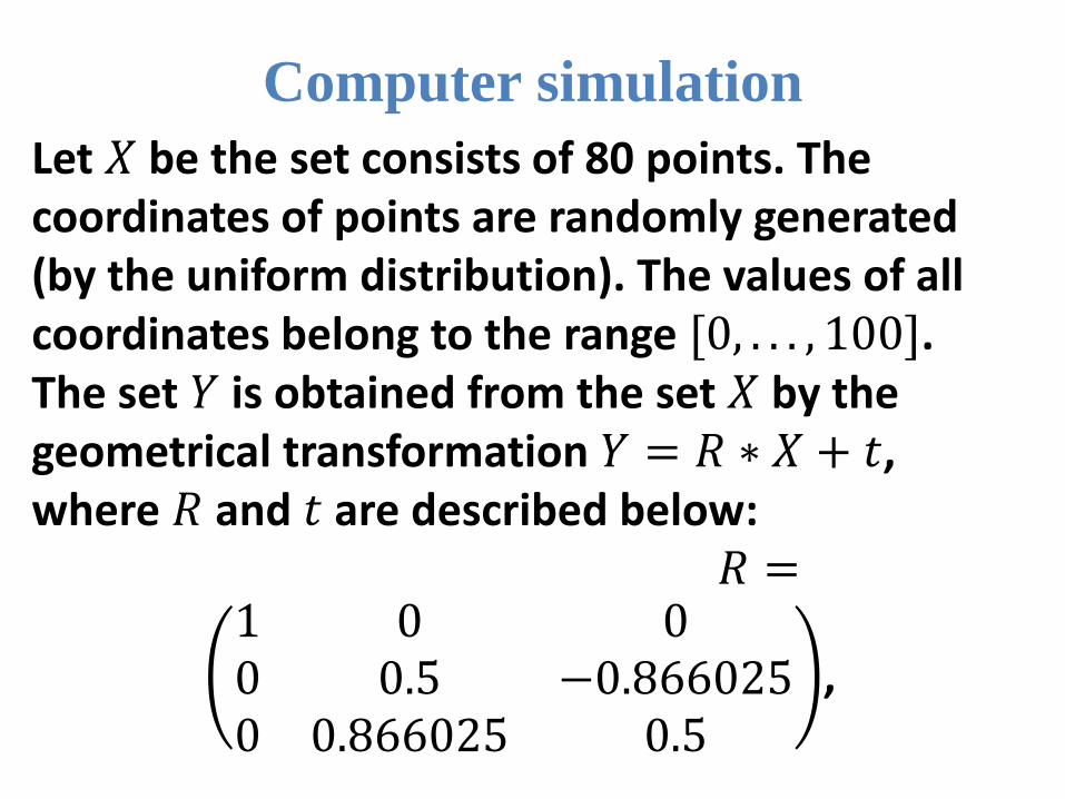
Computer simulation

Let 𝑋 be the set consists of 80 points. The coordinates of points are randomly generated (by the uniform distribution). The values of all coordinates belong to the range [0, . . . , 100]. The set 𝑌 is obtained from the set 𝑋 by the geometrical transformation 𝑌 = 𝑅 ∗ 𝑋 + 𝑡, where 𝑅 and 𝑡 are described below:

𝑅 =1 0 00 0.5 −0.8660250 0.866025 0.5

,

𝑡T = 5 6 7 .

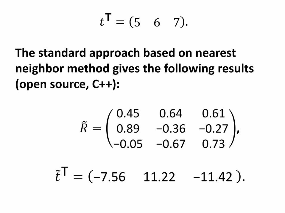
The standard approach based on nearest neighbor method gives the following results(open source, C++):

𝑅 =0.45 0.64 0.610.89 −0.36 −0.27−0.05 −0.67 0.73

,

𝑡T = −7.56 11.22 −11.42 .

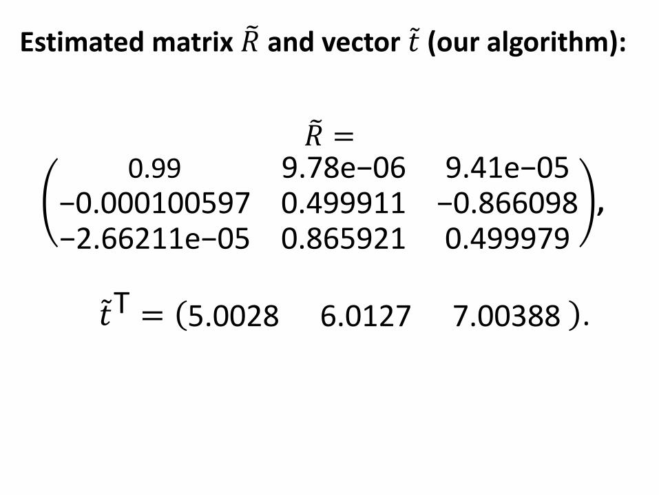
Estimated matrix 𝑅 and vector 𝑡 (our algorithm):

𝑅 =0.99 9.78e−06 9.41e−05

−0.000100597 0.499911 −0.866098−2.66211e−05 0.865921 0.499979

,

𝑡T = 5.0028 6.0127 7.00388 .

Conclusion

In this work we considered matching and error minimizing steps of the ICP algorithm. On the base of the obtained results, a new efficient

algorithm for the sets alignment was designed. The obtained results are illustrated with the

help of computer simulation.