Embed Size (px)
Citation preview

Detection of fashion trends and seasonal cycles through client feedback
KDD 2016 WORKSHOP: MACHINE LEARNING MEETS FASHION
Roberto Sanchis-Ojeda, Daragh Sibley, Paolo Massimi

Contents
1. Intro2. The normal approximation3. Generalized linear mixed effect models4. Application to Stitch Fix’s style feedback data


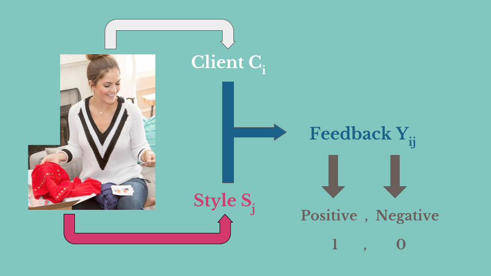
Client Ci
Style Sj
Feedback Yij
Positive , Negative
1 , 0

2. The normal approximation

Simple mathematical law …
Sum of Bernoulli = Binomial
Positive response ratio
Sum of Bernoulli -> Gaussian
pi = ∑j Yij / N
Large N
N = 10 N = 100

… that can be very helpful …
p(time) = 0.7 - 0.2 * time p(time) = 0.5

… but certain assumptions breakLength of every time interval
● Poor temporal resolution
● p no longer constant
● Few interactions, normal approximation breaks
● Slower computation
Large Small

3. Generalized linear mixed effect models

Categorical aggregation
Bernoulli Feedback Yij
0 or 1
Binomial (N0, N1)(34, 27)
logit(p) ~ time + style_color + style_group
Group by each feature to make sure that p is approximately constant within Binomial draw. Now time can be aggregated to an arbitrarily small time scale

Statistical methods with Bernoulli variables
● Pros:
○ Simple, flexible
○ Well studied technique
● Cons:
○ Large dataset
○ Large number of features
○ Scalability problems
● Pros:
○ Smaller dataset
○ Faster computation
○ Natural regularization that helps with non-uniform data
● Cons:
○ Requires a more complex ETL and analysis process.
Logistic Regression Models Generalized Linear Mixed Models

Simulating linear fashion trends
1000 random
styles Si in inventory
Interacting with a large uniform set
of clients
3 interactions per day for
two years with probability pi
pi = pi,o + mi * time
pi,o ~ N(0.6, 0.1) mi ~ U(-0.1, 0.1)

A GLMM linear trend classifier
logit(p) ~ X + Z +
X and Z have an offset and time as featuresThere is a slope per style id, with 95% CI
Out of fashion
CI all negative
Trending
CI all positive

The results

The results
1
2
3
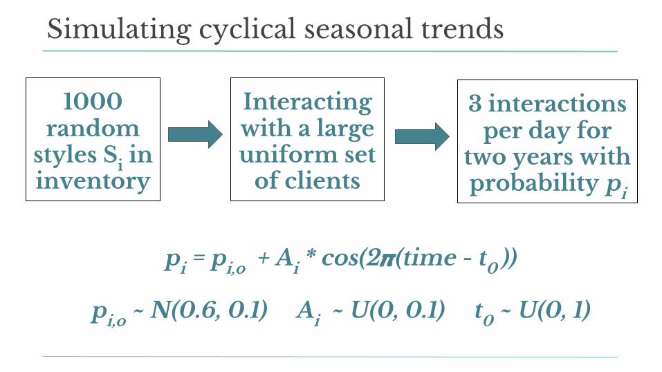
Simulating cyclical seasonal trends
1000 random
styles Si in inventory
Interacting with a large uniform set
of clients
3 interactions per day for
two years with probability pi
pi = pi,o + Ai * cos(2 (time - t0 ))
pi,o ~ N(0.6, 0.1) Ai ~ U(0, 0.1) t0 ~ U(0, 1)

The results

The results
1
2

4. Application to Stitch Fix’s style feedback data

Discovering cyclical seasonal trends
Thousands of real
styles Si in inventory
Interacting with a large uniform set
of clients
Use the style feedback as a probe for seasonality

One great example of seasonal style
Jan Apr July Oct Dec
Conclusions
● Defining client feedback as a binary variable simplifies the statistical analysis of trends
● The normal approximation is a useful tool but lacks the right level of flexibility, and its assumptions are easily broken.
● Binomial data can be fit with generalized linear mixed effect models, and the random effect coefficients can be used to classify trends on styles.
● Our application to Stitch Fix data proves that the method has real business applications.


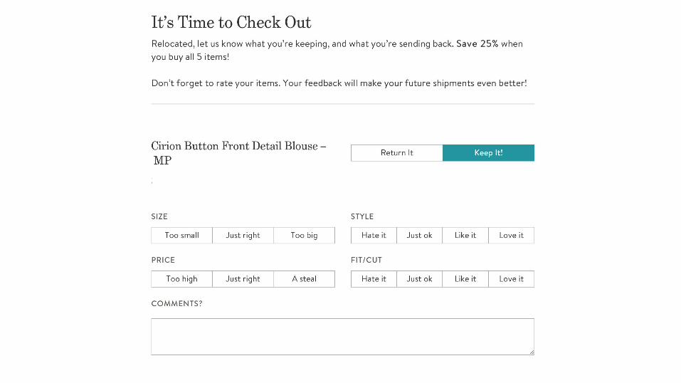
Examples of binarized feedback
● Website feedback:
○ No Click on Picture = Negative = 0
○ Click on Picture = Positive = 1
● Style feedback:
○ (Hate it, Just ok) = Negative = 0
○ (Like it, Love it) = Positive = 1
● Numerical feedback 1, … , N:
○ 1, … , N/2 = Negative = 0
○ N/2, … , N = Positive = 1

Linearizing the cosine term
pi = pi,o + Ai * cos( 2 ( time - t0 ) )
cos( - ) = cos( ) * cos( ) + sin( ) * sin( )
pi = pi,o + Bi * cos( 2 * time ) + Ci * sin( 2 * time )

A GLMM seasonal trend classifier
logit(p) ~ X + Z +
X and Z have an offset and cosine and sine of 2 by time as features
There are two temporal coefficients per style id, with 95% CI
Non-seasonal
CI all comp. with 0 Any other case
Seasonal