Embed Size (px)
Citation preview

Cost Functions
Dr. Andrew McGee
Simon Fraser University

Where we stand…

What we know…
• Production function: (K,L) → Q
• Suppose we know – w = wage rate of L
– R = rental rate of K
• Then we can determine how much it costs for a firm to produce an amount Q=f(K,L) assuming that the firm endeavors to minimize its costs
• That is, we can figure out TC(Q), so all that remains to solve the firm’s profit maximization problem is to determine, P(Q), which depends on market structure
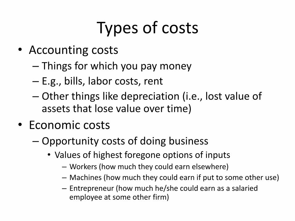
Types of costs• Accounting costs
– Things for which you pay money
– E.g., bills, labor costs, rent
– Other things like depreciation (i.e., lost value of assets that lose value over time)
• Economic costs– Opportunity costs of doing business
• Values of highest foregone options of inputs– Workers (how much they could earn elsewhere)
– Machines (how much they could earn if put to some other use)
– Entrepreneur (how much he/she could earn as a salaried employee at some other firm)

Overlap between Accounting & Economic Costs
• There is significant overlap between accounting & economic costs:– E.g., labor costs=wages=opportunity cost of labor in a
competitive labor market
• Economic costs > accounting costs– Entrepreneur’s salary < opportunity costs because
entrepreneur receives a large share of firm’s accounting profits as owner of firm
– Investors’ opportunity costs are not reflected in firm’s costs (compensated through accounting profits by way of dividends, capital gains)
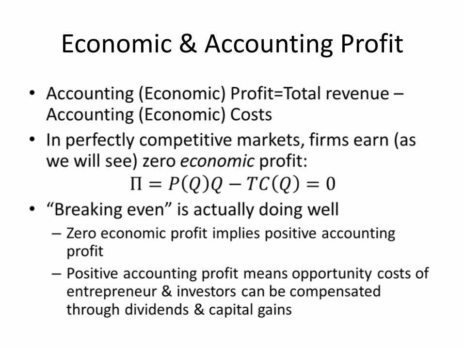
Economic & Accounting Profit

Economic Costs (forget about accounting costs for now)
w r
L K
Price-takers in input markets

Deriving Total Cost Function

Cost Minimization Problem

Cost Minimization

Example

Cost minimization

A
Depicting Cost MinimizationK
L
q0
Isocost or isoexpenditure lines
-w/r
IsoquantTC0=rK0
TC1=rK1
TC2=rK2
w/r=MRTS
TC3=rK3 All input combinations on the iso-expenditure (iso-cost) lines are input combinations that result in the same total cost of production
Total cost is declining in the southwesterly direction
This firm can produce q0 for less than TC3, but it cannot produce q0 for TC1 or TC2. Notice that for this and every output level and given input prices (w & r) there is a unique minimum cost of production.Our goal is to derive TC(w,r,q)

Duality: Output maximization
• For every constrained maximization problem there exists a constrained minimization problem yielding the same solution for appropriate parameter values (“duality”)
• Dual problem of cost minimization: maximize output subject to expenditure constraint

Output MaximizationK
Lq0
A
E=rK
q3
q2
q1
w/r=MRTS
E=wL
Solving the Lagrangian will yield the same optimal condition: w/r=MRTS

Demand for inputs?K
q0
q3
q2
q1 L
A
Demand for L at different wage rates? NO!

Demand for inputs?
• Can we derive firm’s demand for inputs (K,L) using solutions to cost minimization problem (much like we derived demand for goods using the solution to the consumer choice problem)?
• No!
• Cost minimization holds output constant, but firm’s demand for K & L obviously depends on how much output it chooses to produce.

Deriving Total Cost FunctionK
L
TC0=rK0
TC1=rK1
TC2=rK2
TC3=rK3 Cost expansion path: from this expansion path we can obtain the TC associated with each output level q
q0
q3q2
q1
q E
q0
q1
q2
q3 TC3
TC2
TC1
TC0
TC(w,r,q)
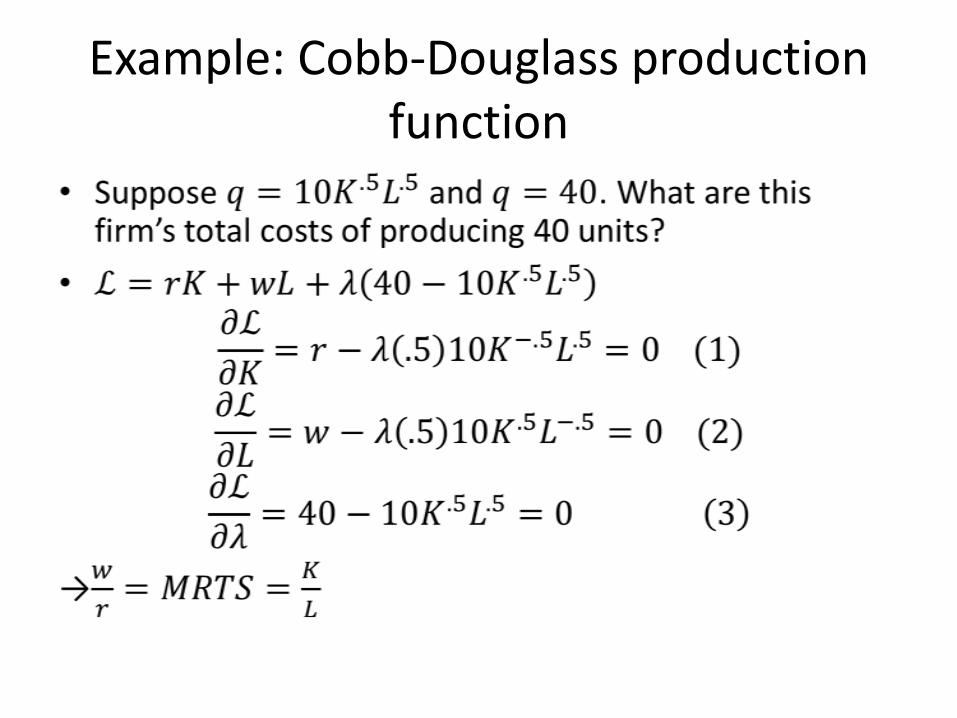
Example: Cobb-Douglass production function

Example: Cobb-Douglass production function
• →wL=rK
• Suppose w=r=$4. Then L=K. If L=K & q=40, we have
• This implies that TC=$4*4+$4*4=$32 (lowest possible cost of producing 40 units)
• &
• (extra output for last $1 spent on inputs)

Example: Cobb-Douglass production function

Example: Deriving the Cost Function for a Cobb-Douglass production function
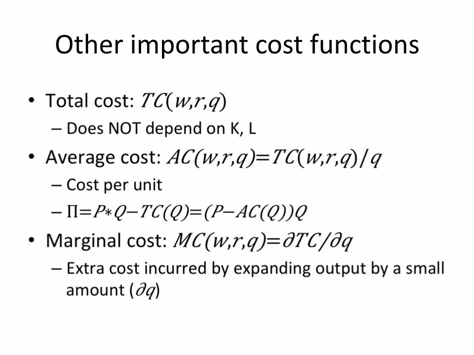
Other important cost functions
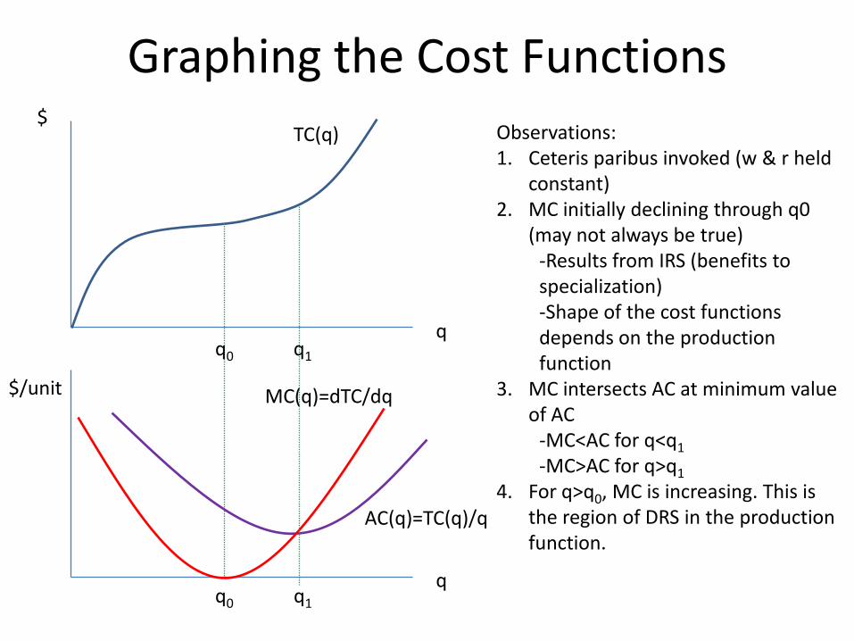
Graphing the Cost Functions
q
q
$
$/unit
TC(q)
AC(q)=TC(q)/q
MC(q)=dTC/dq
q0
q0
q1
q1
Observations:1. Ceteris paribus invoked (w & r held
constant)2. MC initially declining through q0
(may not always be true)-Results from IRS (benefits to specialization)-Shape of the cost functions depends on the production function
3. MC intersects AC at minimum value of AC
-MC<AC for q<q1
-MC>AC for q>q1
4. For q>q0, MC is increasing. This is the region of DRS in the production function.

Example: Deriving MC and AC functions

CRS production functions & cost functions
q
$TC(q)
IRS CRS DRS
CRS production functions have linear TC functions because MC is constant:
$TC(q)
q

CRS production functions & cost functions
• What is AC when production function exhibits CRS everywhere? In previous example and in all such examples, AC(q)=TC(q)/q=c, a constant.
q
$/unit
AC=MC
When f(K,L) exhibits CRS everywhere, AC(q)=MC(q)=constant. When you see constant marginal costs, you immediately know something about the productions function. Likewise, when you see CRS, you immediately know something about the MC>

Effects of input price increase
• When the price of one of the two inputs goes up, what happens if producers wish to maintain the same level of output?
– Producers will substitute the now relatively cheaper input for some of the input whose price increased
– Total costs definitely do not decrease following an input price increase. If they do, the producer could not have been minimizing costs to start with

Partial elasticity of substitution between inputs

Partial elasticity of substitution between inputs
• Partial elasticity of substitution (s) measures how firms change input mix in response to price changes
• High s → firms change input mix (K/L ratio) substantially in response to small changes in relative input prices
• Low s → firms change input mix (K/L ratio) little in response to changes in relative input prices

Long vs. Short Run Costs
• Short run = period of time during which at least one input cannot be changed
• Long run = any time horizon during which allinput can be changed
• Variable input = input that can be changed in the short run
• Fixed input = input that cannot be changed in the short run– Some inputs take time to be delivered or made; this
time-to-delivery defines the short run
• All inputs are variable in the long run

Short run cost functions

Short run cost functions

Enveloping the Short-run cost curves
• Envelope of the STC: The set of lowest costs of production on any STC (i.e., for any fixed level of K) for every possible output level
• The envelope of the STC curves defines the TC curve
• Similarly, the envelope of the SATC curves defines the AC curve

Enveloping the Short-run cost curves
TC
q
TC(w,r,q)
Imagine that each STC curve corresponds to the firm’s cost schedule with a different number of plants. How many plants should the firm build to produce q1, q2, q3, and q4 units of output?
q1q2 q3 q4
This TC curve is linear. What does that tell us?

Enveloping the Short-run cost curves
The envelope of the STC curves need not be linear.
TC
q
TC
q1q2 q3 q4
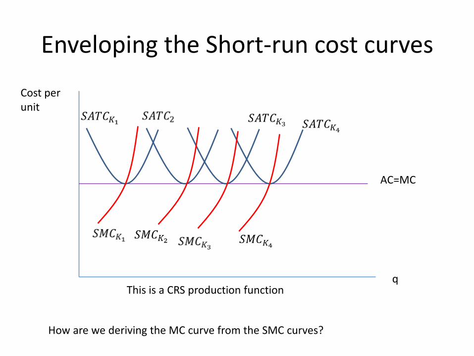
Enveloping the Short-run cost curves
q
Cost per unit
AC=MC
This is a CRS production function
How are we deriving the MC curve from the SMC curves?

Enveloping the Short-run cost curves
q
Cost per unit
AC
MC
For each output level, find the SMC curve corresponding to the SATC just tangent to the AC curve. From this SMC curve we derive the MC (in the LR) of producing that output level.
MES=minimum efficient scale
At MES, AC reaches its minimum values and AC=MC=SATC=SMC
Not CRS

Example: Short run Cobb Douglass Costs
Fixed input STC
=1
=4
=9

Example: Short run Cobb Douglass Costs
• If in the short run you happen to be using the capital level that minimizes the costs of producing output level q in the long run (K1*), then you must also be minimizing costs in the short run, meaning that the derivative of the STC at this capital level is zero. Use this fact to solve for K1*:
• Plug this back into the STC. You are now effectively using the K level that minimizes LR costs while using the L-level that minimizes costs for any given K-level. Thus you must be minimizing costs in the LR, so this is the TC function:
• You can check that this is indeed the same as the TC we derived earlier for this Cobb Douglass production function