1

Chapter 5 – Traverse

Horizontal Control Surveys One of the first steps in construction project is to establish a network of both vertical and horizontal control points on or near the ground in the vicinity of the project. The relative positions of all the points are accurately determined in a control survey. The control points serve as fixed reference positions from which other surveying measurements are made later on to design and build the project.

A horizontal control network may be established by one or a combination of the following methods: (1) Traversing

i. A traverse survey involves a connected sequence of lines whose length and directions are measured.

ii. It is perhaps the most common type of control survey performed by surveyors in private practice or employed by local governmental agencies.

iii. Precise traverse surveys are much more practical nowadays with the use of electronic distance measuring (EDM) devices.

(2) Triangulation i. Involves a system of joined or overlapping triangles in which the lengths of two

sides (called baselines) are measured. ii. The other sides are then computed from the angles measured at the triangle

vertices. iii. This is the best method used in the past to establish precise horizontal control over

large areas because precise angular measurement was more feasible than precise distance measurement by taping.

(3) Trilateration

i. Involves a system of triangles but only the lengths are measured.

Traverse

A traverse is usually a control survey and is employed in all forms of legal, mapping, and engineering surveys. A traverse consists of an interconnected series of lines called courses, running between a series of points on the ground called traverse stations. A traverse is a series of established stations tied together by angle and distance.

2

The angles are measured using theodolites, or total stations, whereas the distances can be measured using total stations, steel tapes or electronic distance-measurement instruments (EDMs). In engineering work, traverses are used as control surveys to:

1. Locate topographic detail for the preparation of plans 2. Lay out (locate) engineering works 3. Process and order earthwork and other engineering quantities.

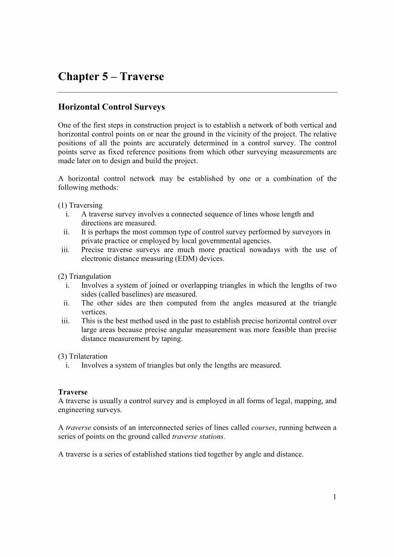
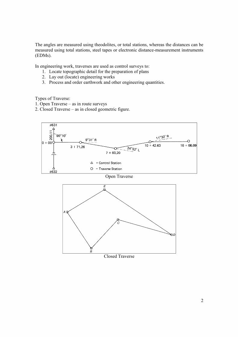
Types of Traverse: 1. Open Traverse – as in route surveys 2. Closed Traverse – as in closed geometric figure.

Open Traverse

Closed Traverse

3

Open Traverse

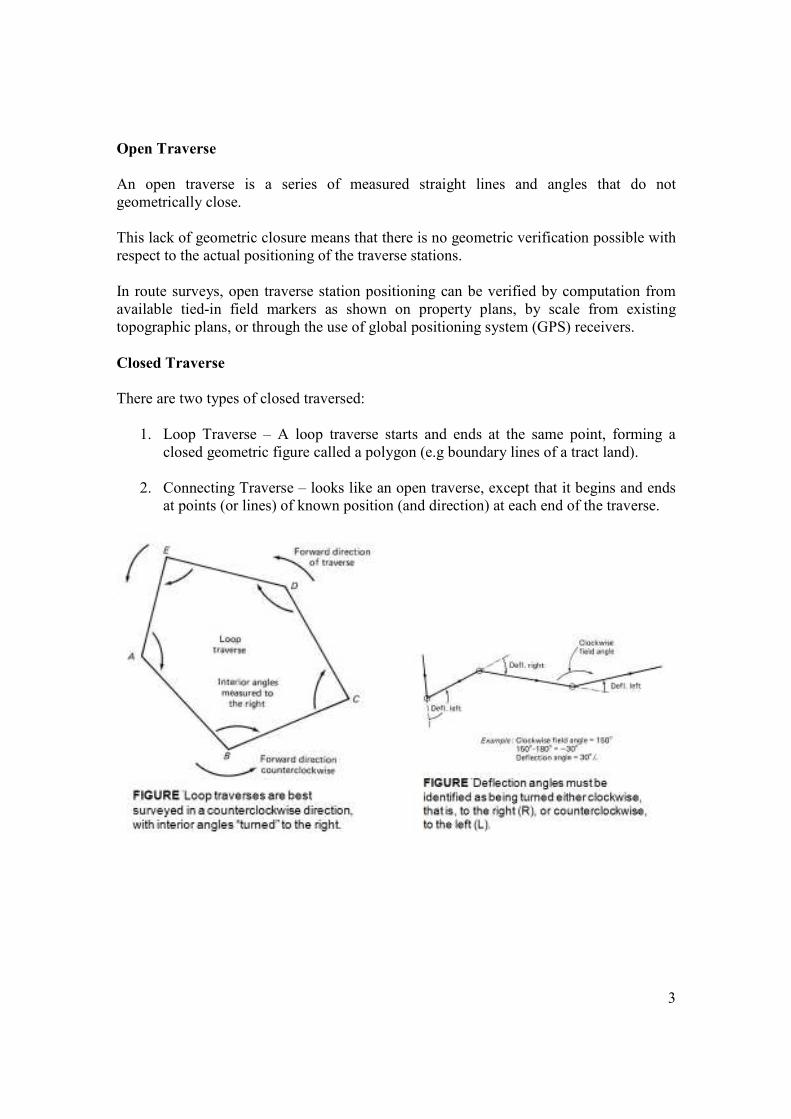
An open traverse is a series of measured straight lines and angles that do not geometrically close. This lack of geometric closure means that there is no geometric verification possible with respect to the actual positioning of the traverse stations. In route surveys, open traverse station positioning can be verified by computation from available tied-in field markers as shown on property plans, by scale from existing topographic plans, or through the use of global positioning system (GPS) receivers. Closed Traverse

There are two types of closed traversed:

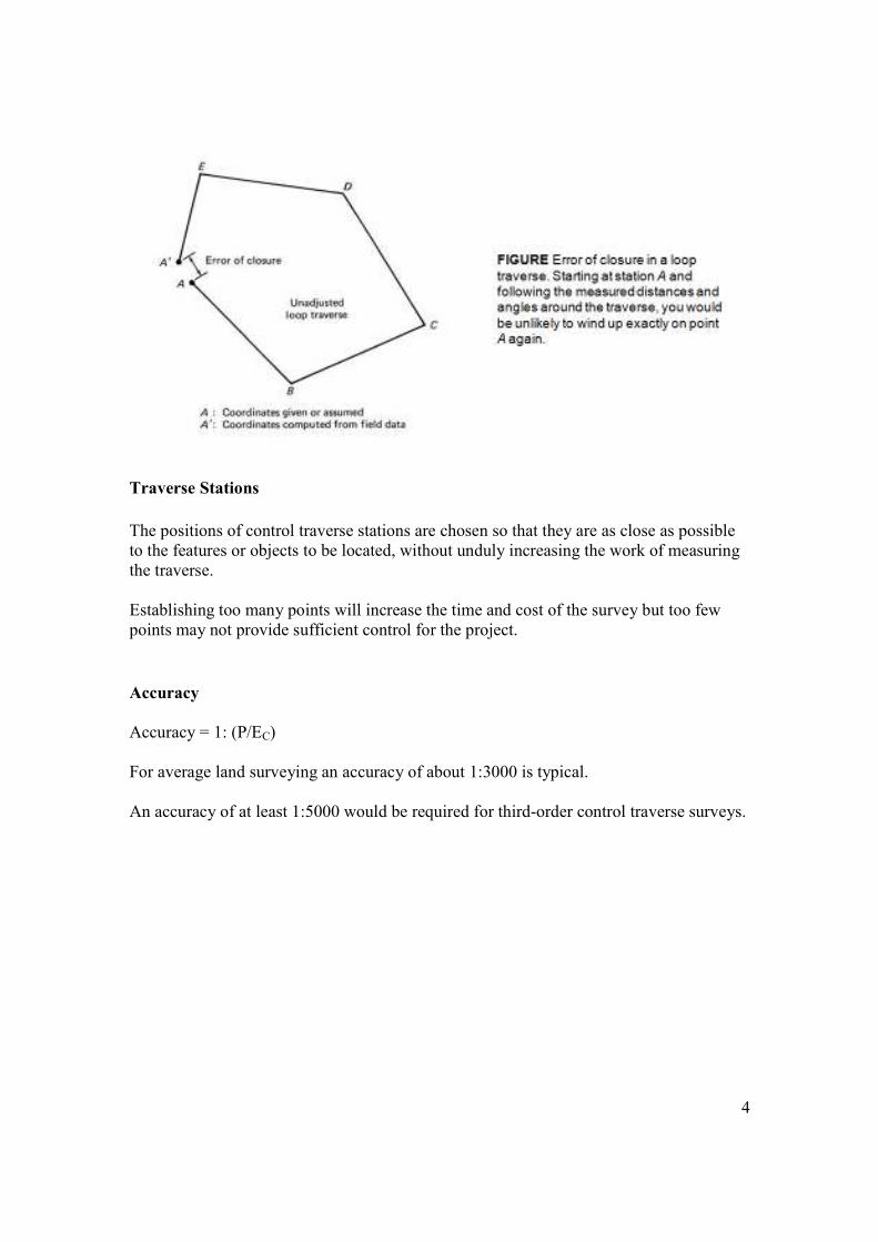
1. Loop Traverse – A loop traverse starts and ends at the same point, forming a closed geometric figure called a polygon (e.g boundary lines of a tract land).

2. Connecting Traverse – looks like an open traverse, except that it begins and ends at points (or lines) of known position (and direction) at each end of the traverse.

4

Traverse Stations

The positions of control traverse stations are chosen so that they are as close as possible to the features or objects to be located, without unduly increasing the work of measuring the traverse. Establishing too many points will increase the time and cost of the survey but too few points may not provide sufficient control for the project.

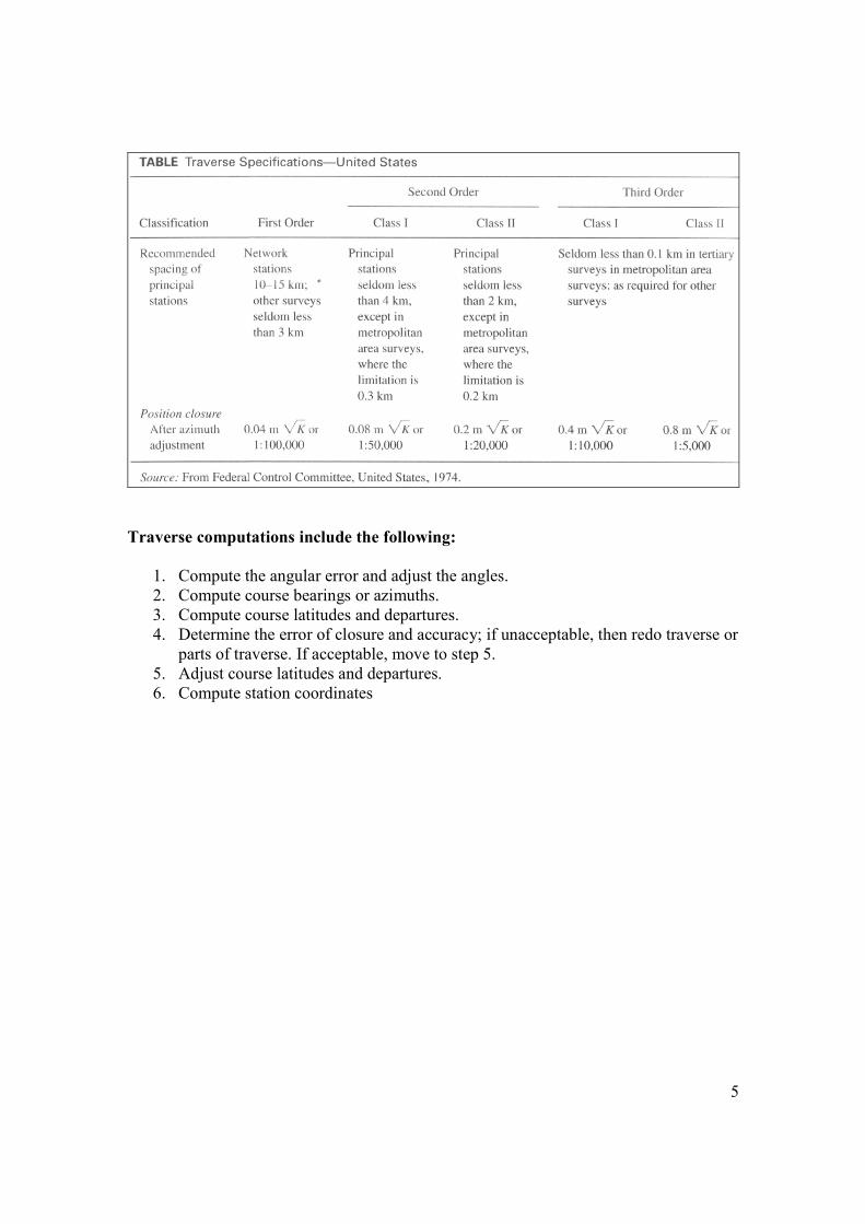
Accuracy

Accuracy = 1: (P/EC) For average land surveying an accuracy of about 1:3000 is typical. An accuracy of at least 1:5000 would be required for third-order control traverse surveys.

5

Traverse computations include the following:

1. Compute the angular error and adjust the angles. 2. Compute course bearings or azimuths. 3. Compute course latitudes and departures. 4. Determine the error of closure and accuracy; if unacceptable, then redo traverse or

parts of traverse. If acceptable, move to step 5. 5. Adjust course latitudes and departures. 6. Compute station coordinates

6

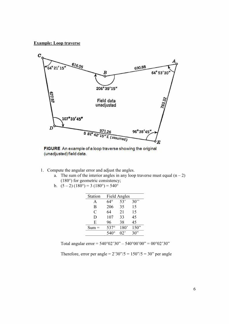
Example: Loop traverse

1. Compute the angular error and adjust the angles. a. The sum of the interior angles in any loop traverse must equal (n – 2)

(180°) for geometric consistency; b. (5 – 2) (180°) = 3 (180°) = 540°

Station Field Angles

A 64° 53’ 30’’ B 206 35 15 C 64 21 15 D 107 33 45 E 96 38 45

Sum = 537° 180’ 150” 540° 02’ 30”

Total angular error = 540°02’30” – 540°00’00” = 00°02’30” Therefore, error per angle = 2’30”/5 = 150”/5 = 30” per angle

7

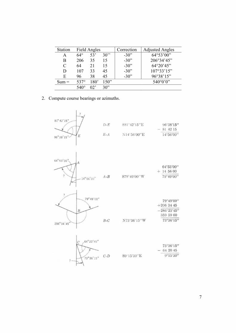
Station Field Angles Correction Adjusted Angles

A 64° 53’ 30’’ -30” 64°53’00” B 206 35 15 -30” 206°34’45” C 64 21 15 -30” 64°20’45” D 107 33 45 -30” 107°33’15” E 96 38 45 -30” 96°38’15”

Sum = 537° 180’ 150” 540°0’0” 540° 02’ 30”

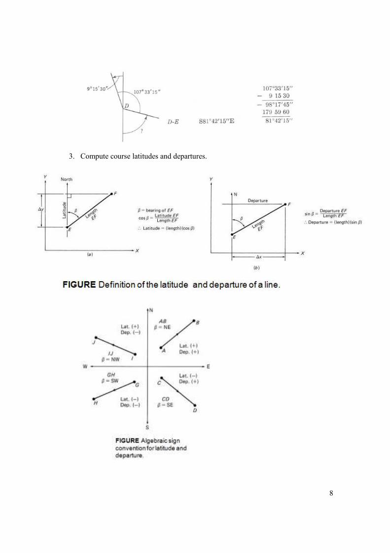
2. Compute course bearings or azimuths.

8

3. Compute course latitudes and departures.

9

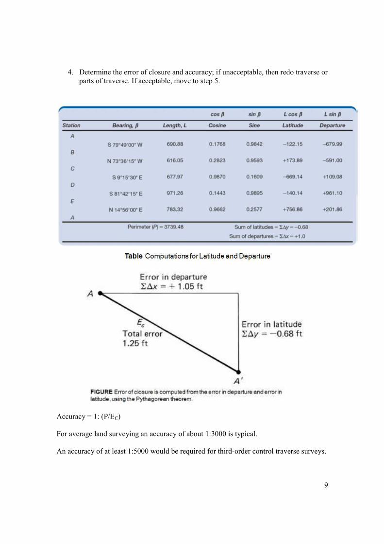
4. Determine the error of closure and accuracy; if unacceptable, then redo traverse or parts of traverse. If acceptable, move to step 5.

Accuracy = 1: (P/EC) For average land surveying an accuracy of about 1:3000 is typical. An accuracy of at least 1:5000 would be required for third-order control traverse surveys.

10

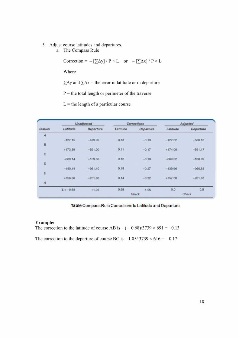
5. Adjust course latitudes and departures. a. The Compass Rule

Correction = – [∑∆y] / P × L or – [∑∆x] / P × L Where ∑∆y and ∑∆x = the error in latitude or in departure P = the total length or perimeter of the traverse L = the length of a particular course

Example:

The correction to the latitude of course AB is – ( – 0.68)/3739 × 691 = +0.13 The correction to the departure of course BC is – 1.05/ 3739 × 616 = – 0.17

11

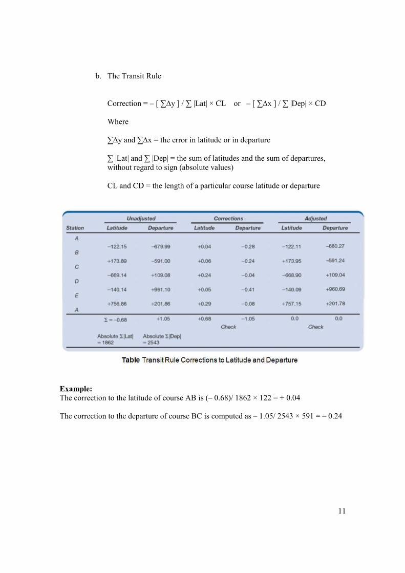
b. The Transit Rule

Correction = – [ ∑∆y ] / ∑ |Lat| × CL or – [ ∑∆x ] / ∑ |Dep| × CD Where ∑∆y and ∑∆x = the error in latitude or in departure ∑ |Lat| and ∑ |Dep| = the sum of latitudes and the sum of departures, without regard to sign (absolute values) CL and CD = the length of a particular course latitude or departure

Example:

The correction to the latitude of course AB is (– 0.68)/ 1862 × 122 = + 0.04 The correction to the departure of course BC is computed as – 1.05/ 2543 × 591 = – 0.24

12

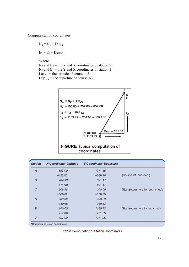
Compute station coordinates

N2 = N1 + Lat1-2 E2 = E1 + Dep1-2 Where N2 and E2 = the Y and X coordinates of station 2 N1 and E1 = the Y and X coordinates of station 1 Lat 1-2 = the latitude of course 1-2 Dep 1-2 = the departure of course 1-2

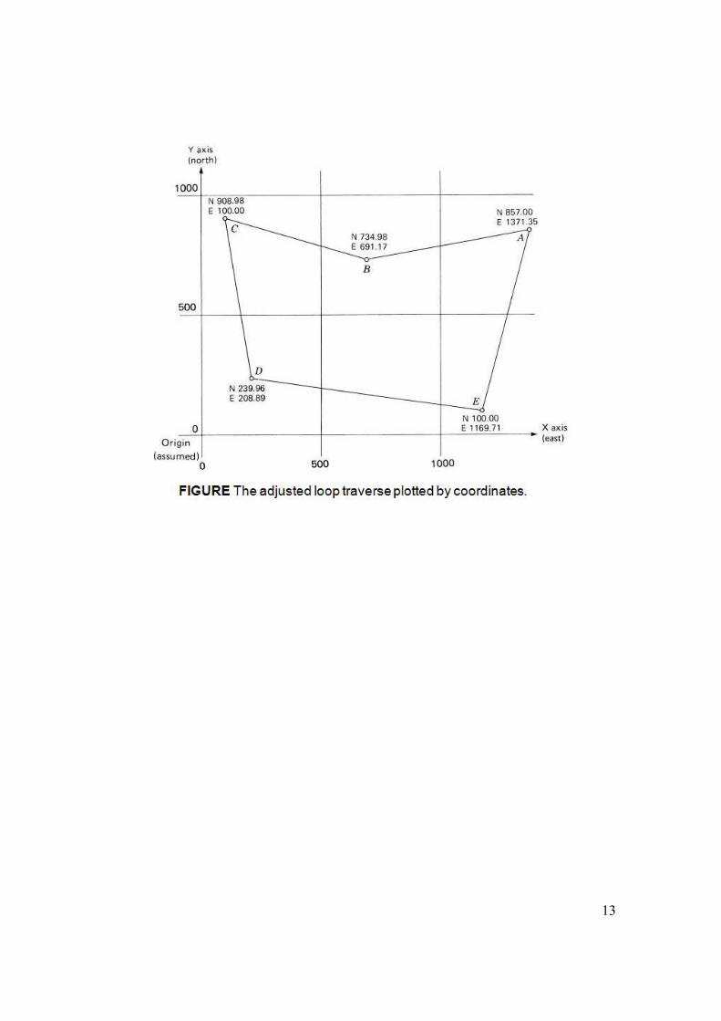
13

14

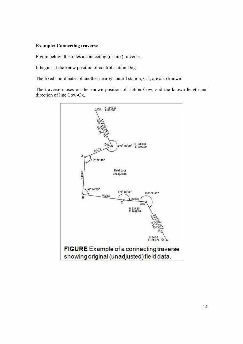
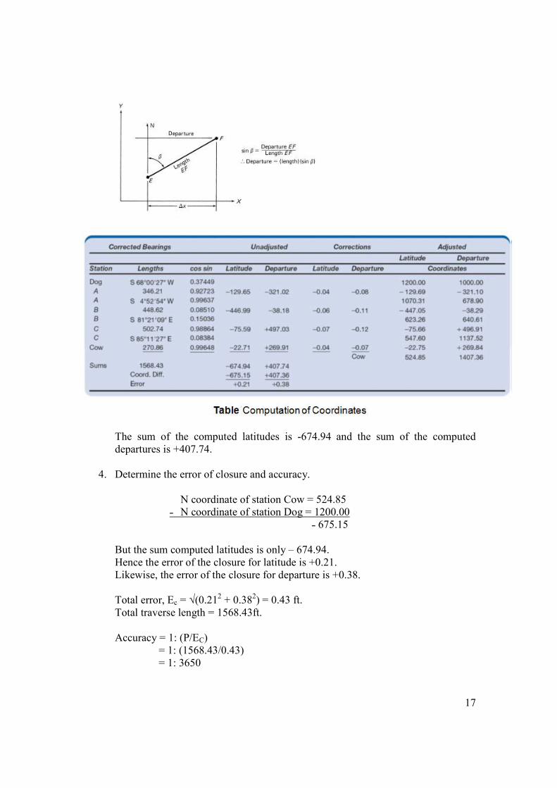
Example: Connecting traverse

Figure below illustrates a connecting (or link) traverse. It begins at the know position of control station Dog. The fixed coordinates of another nearby control station, Cat, are also known. The traverse closes on the known position of station Cow, and the known length and direction of line Cow-Ox.

15

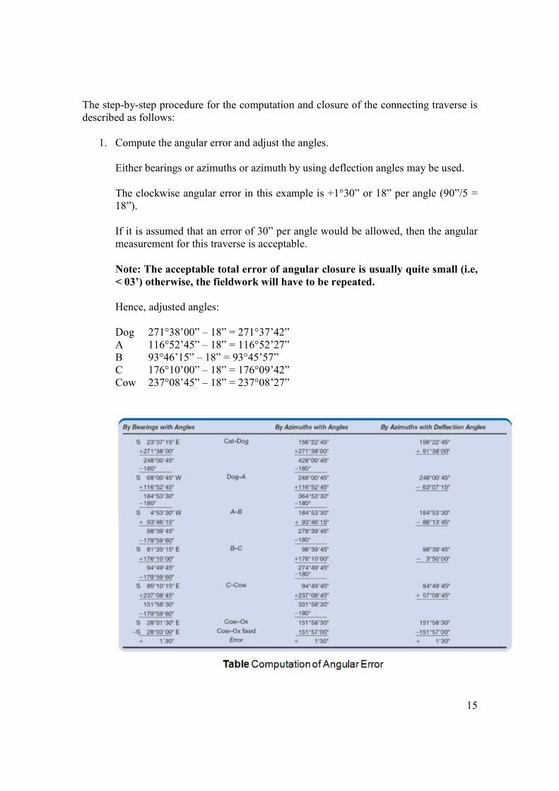
The step-by-step procedure for the computation and closure of the connecting traverse is described as follows:

1. Compute the angular error and adjust the angles. Either bearings or azimuths or azimuth by using deflection angles may be used. The clockwise angular error in this example is +1°30” or 18” per angle (90”/5 = 18”). If it is assumed that an error of 30” per angle would be allowed, then the angular measurement for this traverse is acceptable. #ote: The acceptable total error of angular closure is usually quite small (i.e,

< 03’) otherwise, the fieldwork will have to be repeated.

Hence, adjusted angles: Dog 271°38’00” – 18” = 271°37’42” A 116°52’45” – 18” = 116°52’27” B 93°46’15” – 18” = 93°45’57” C 176°10’00” – 18” = 176°09’42” Cow 237°08’45” – 18” = 237°08’27”

16

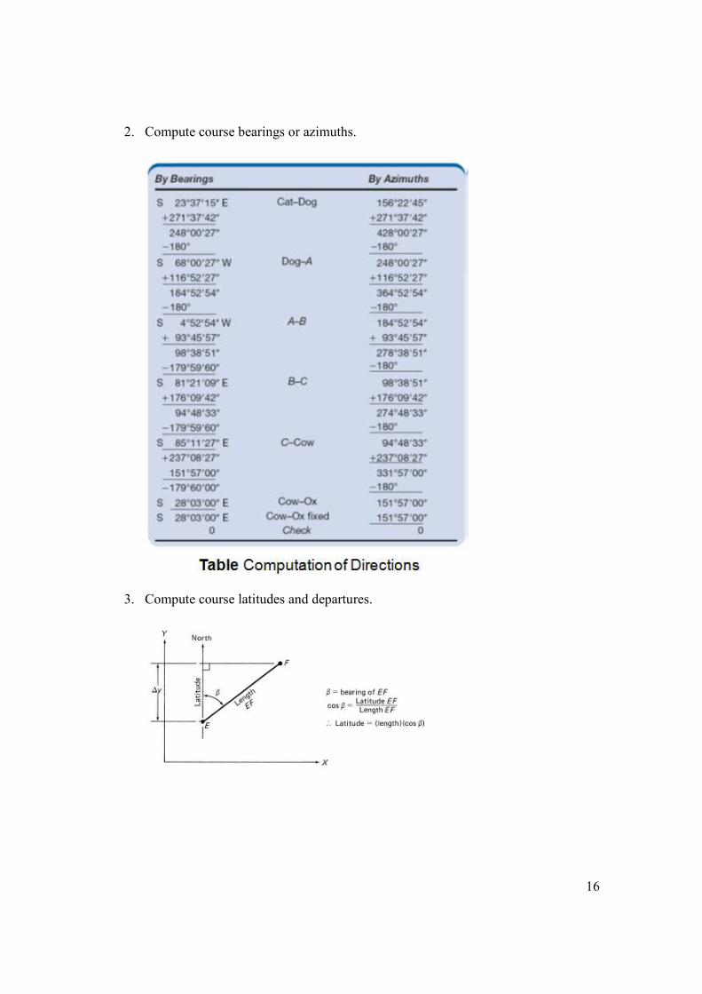
2. Compute course bearings or azimuths.

3. Compute course latitudes and departures.

17

The sum of the computed latitudes is -674.94 and the sum of the computed departures is +407.74.

4. Determine the error of closure and accuracy.

N coordinate of station Cow = 524.85 ˗ N coordinate of station Dog = 1200.00

˗ 675.15 But the sum computed latitudes is only – 674.94. Hence the error of the closure for latitude is +0.21. Likewise, the error of the closure for departure is +0.38. Total error, Ec = √(0.212 + 0.382) = 0.43 ft. Total traverse length = 1568.43ft. Accuracy = 1: (P/EC) = 1: (1568.43/0.43) = 1: 3650

18

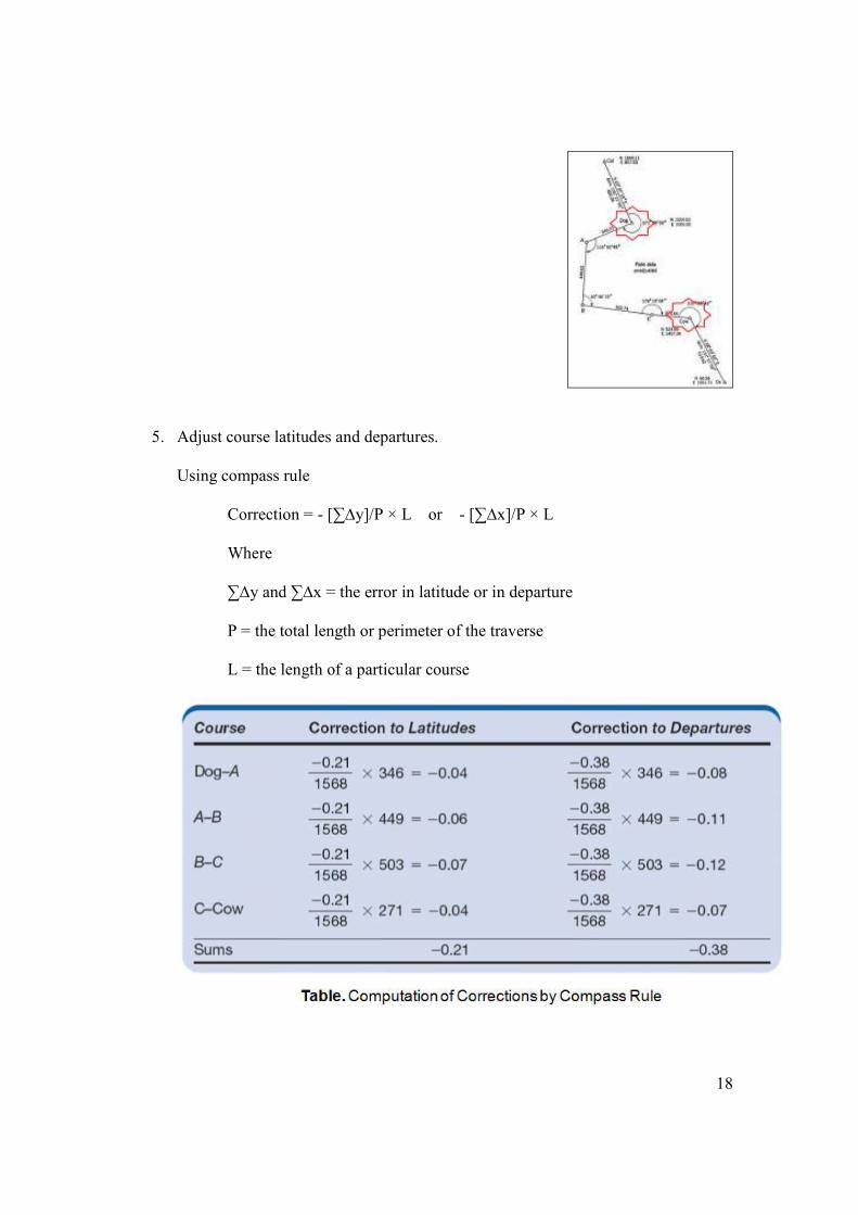
5. Adjust course latitudes and departures. Using compass rule

Correction = - [∑∆y]/P × L or - [∑∆x]/P × L Where ∑∆y and ∑∆x = the error in latitude or in departure P = the total length or perimeter of the traverse L = the length of a particular course

19

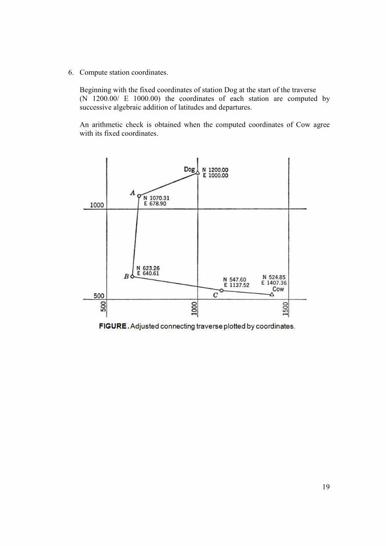
6. Compute station coordinates. Beginning with the fixed coordinates of station Dog at the start of the traverse (N 1200.00/ E 1000.00) the coordinates of each station are computed by successive algebraic addition of latitudes and departures. An arithmetic check is obtained when the computed coordinates of Cow agree with its fixed coordinates.

20

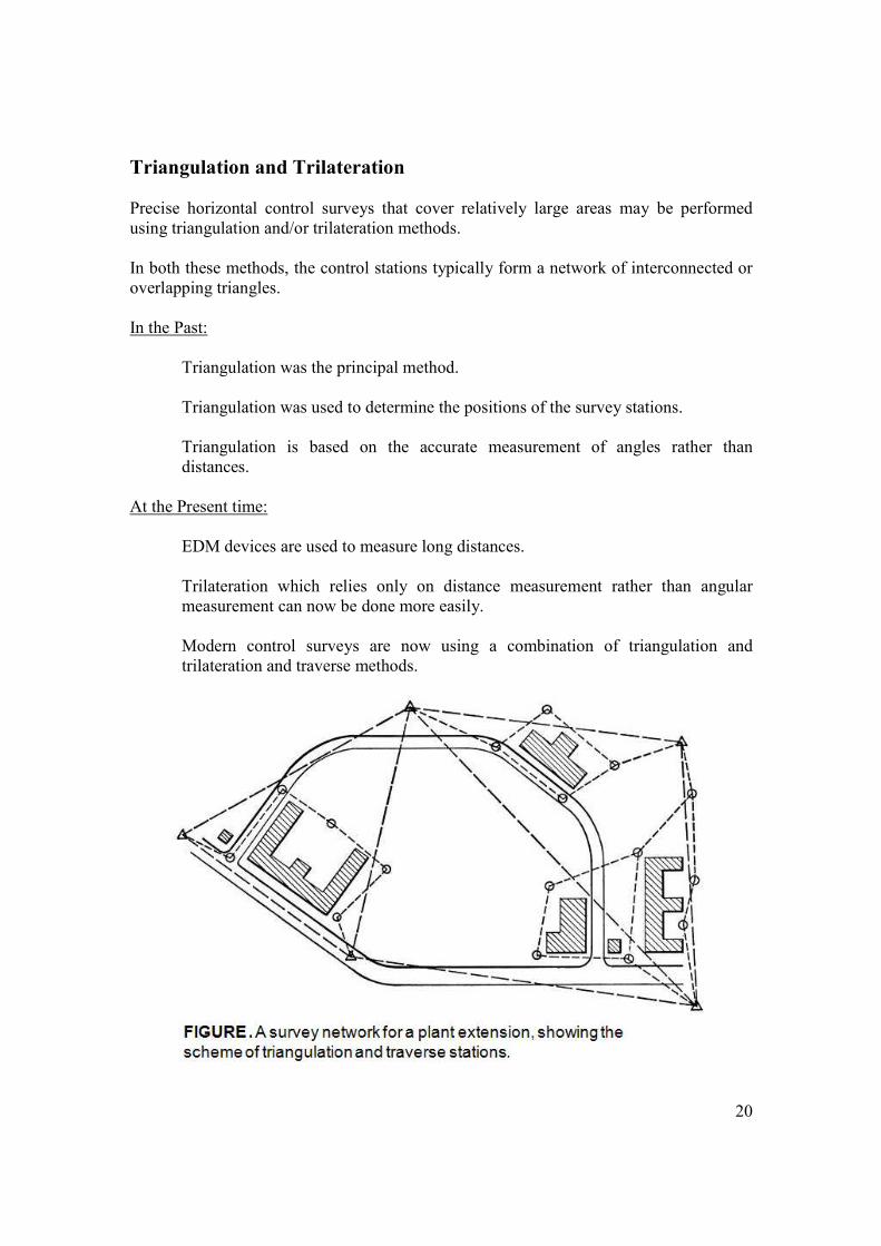
Triangulation and Trilateration Precise horizontal control surveys that cover relatively large areas may be performed using triangulation and/or trilateration methods. In both these methods, the control stations typically form a network of interconnected or overlapping triangles. In the Past:

Triangulation was the principal method. Triangulation was used to determine the positions of the survey stations. Triangulation is based on the accurate measurement of angles rather than distances.

At the Present time:

EDM devices are used to measure long distances. Trilateration which relies only on distance measurement rather than angular measurement can now be done more easily. Modern control surveys are now using a combination of triangulation and trilateration and traverse methods.

21

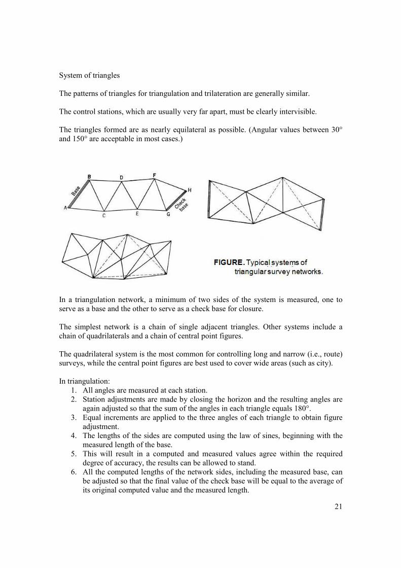
System of triangles The patterns of triangles for triangulation and trilateration are generally similar. The control stations, which are usually very far apart, must be clearly intervisible. The triangles formed are as nearly equilateral as possible. (Angular values between 30° and 150° are acceptable in most cases.)

In a triangulation network, a minimum of two sides of the system is measured, one to serve as a base and the other to serve as a check base for closure. The simplest network is a chain of single adjacent triangles. Other systems include a chain of quadrilaterals and a chain of central point figures. The quadrilateral system is the most common for controlling long and narrow (i.e., route) surveys, while the central point figures are best used to cover wide areas (such as city). In triangulation:

1. All angles are measured at each station. 2. Station adjustments are made by closing the horizon and the resulting angles are

again adjusted so that the sum of the angles in each triangle equals 180°. 3. Equal increments are applied to the three angles of each triangle to obtain figure

adjustment. 4. The lengths of the sides are computed using the law of sines, beginning with the

measured length of the base. 5. This will result in a computed and measured values agree within the required

degree of accuracy, the results can be allowed to stand. 6. All the computed lengths of the network sides, including the measured base, can

be adjusted so that the final value of the check base will be equal to the average of its original computed value and the measured length.

22

In trilateration:

1. Only the distances between control stations are measured (using EDM). 2. Horizontal angular measurements are unnecessary. 3. The angles are computed using the law of cosines.

� a2 = b 2 + c 2 - 2bc Cos A � b2 = a2 + c2 - 2 ac Cos B � c2 = a2 + b2 – 2ab Cos C

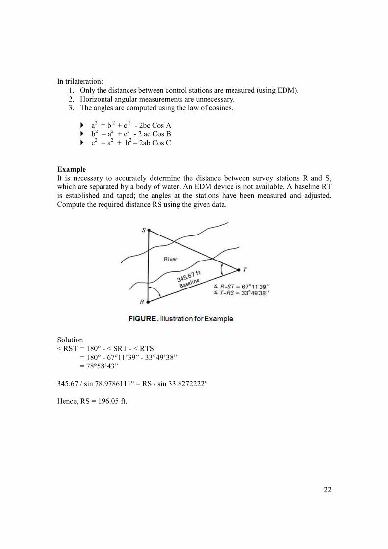
Example

It is necessary to accurately determine the distance between survey stations R and S, which are separated by a body of water. An EDM device is not available. A baseline RT is established and taped; the angles at the stations have been measured and adjusted. Compute the required distance RS using the given data.

Solution < RST = 180° - < SRT - < RTS = 180° - 67°11’39” - 33°49’38” = 78°58’43” 345.67 / sin 78.9786111° = RS / sin 33.8272222° Hence, RS = 196.05 ft.

23

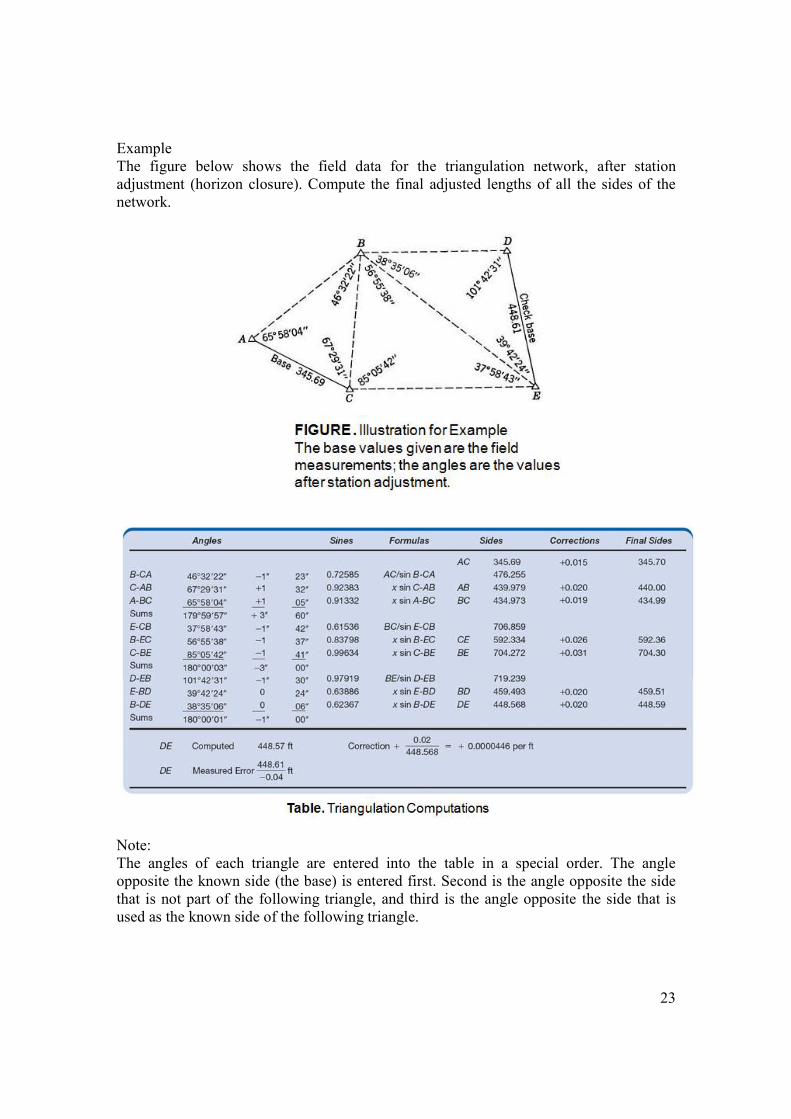
Example The figure below shows the field data for the triangulation network, after station adjustment (horizon closure). Compute the final adjusted lengths of all the sides of the network.

Note: The angles of each triangle are entered into the table in a special order. The angle opposite the known side (the base) is entered first. Second is the angle opposite the side that is not part of the following triangle, and third is the angle opposite the side that is used as the known side of the following triangle.